Comment on Choi et al. Correlation between Ionospheric TEC and the DCB Stability of GNSS Receivers from 2014 to 2016. Remote Sens. 2019, 11, 2657

Abstract

Choi et al. (2019) analyzed the correlation between the ionospheric total electron content (TEC) and the Global Navigation Satellite System (GNSS) receiver differential code bias (DCB) and concluded that the long-term variations of the receiver DCB are caused by the corresponding variations in the ionosphere. Unfortunately, their method is problematic, resulting in conclusions that are not useful. The long-term variations of the Global Positioning System (GPS) DCBs are primarily attributed to the GPS satellite replacement with different satellite block series under the zero-mean constraint condition, rather than the ionospheric variability.

In the ionospheric total electron content (TEC) retrieval, the differential code bias (DCB) caused by the Global Navigation Satellite System (GNSS) satellite transmitter and receiver hardware is one of the main error sources, and it has been widely studied. Choi et al. [1] have recently proposed a new aspect of the correlation between the ionospheric TEC and the GNSS receiver differential code bias (rDCB). They stated that “the characteristics of rDCB and rDCB root mean square (RMS) have a similarity with those of vertical TEC (VTEC), at all stations”, and they calculated Pearson’s coefficient (R) between the TEC and rDCB and showed that “the correlation between TEC and rDCB is the smallest in low-latitude regions. The mid-latitude regions exhibit the maximum value of R”. Supposedly, the GNSS DCB should be related with the transmitter hardware and its environment, as expected. Studies also showed that the variations of the Global Positioning System (GPS) satellite DCB and receiver DCB are not caused by the ionospheric variability [2,3]. However, Choi et al. [1] might have advertently or inadvertently overlooked the work of Zhong et al. [2,3]. As discussed subsequently, it does not make sense to utilize the comparison between the ionospheric TEC and the GNSS receiver DCB to demonstrate their cause–effect relationship. Thus, the correlation analysis between TEC and rDCB as described by Choi et al. [1] is not meaningful.

Zhong et al. [2,3] have assessed the variations of the GPS satellite DCB and receiver DCB. Note that in the DCB estimation, only the combined satellite–receiver DCB (the sum of the GPS DCB and receiver DCB) can actually be determined, so that an additional constraint condition is required to further separate the GPS DCB and receiver DCB. Generally, the zero-mean condition imposed on all satellite DCBs (i.e., the daily mean of all GPS DCBs is set as zero) is introduced for the DCB separation [4]. Figure 1 shows the comparisons of the GPS DCB of Pseudo Random Number (PRN) 13 from the International GNSS Service (IGS) [5] and solar activity proxy F10.7 during 1998–2020. It seems that the GPS DCB also showed a solar-cycle-like variation [6], if only the period of 2002–2014 is considered. However, this is not the case for the whole period of 1998–2020.

Figure 2 presents the lifetime of each GPS satellite from 1998 to 2020. It is clear that the new satellite block series are replacing the old ones gradually. From the GPS DCB values on 1 January 2015 as displayed at the upper left corner of Figure 2, it is evident that the GPS DCBs from different satellite block series show a significant difference. Under the zero-mean condition imposed on all GPS DCBs, when a new GPS satellite replaces a decommissioned one with a different block series, the GPS DCB values change relatively to satisfy the zero-mean condition. Specifically, when a new GPS satellite with higher (lower) DCB values comes into service, all the GPS DCB values descend (increase). Thus, the long-term variations of the GPS DCBs are not caused by the ionospheric variability, while they are attributed to the GPS satellite replacement with different satellite block series under the zero-mean condition [2]. Correspondingly, the estimated receiver DCB will also change, as the daily combined satellite–receiver DCB is constant. Note that only after the effect of GPS satellite replacement is removed, the DCB could be used for comparison or periodic spectral analysis.

To remove the effect of GPS satellite replacement, we can reconstruct the DCB value under a new constraint condition imposed only on continuously operating GPS satellites during a specific period. The new constraint condition for the GPS DCBs is expressed as follows:

$$\frac{1}{n}{\displaystyle {\sum }_{i=1}^{n}DC{B}_{\mathrm{s},\mathrm{rec}}^i}=\mathrm{C}$$

(1)

where DCB_s,rec denotes the reconstructed GPS DCB, n is the number of the selected GPS satellites, and C is a constant value. During the period of 2005–2019, nine continuously operating GPS satellites (PRN 11, 13, 14, 16, 19, 20, 22, 23, and 28) are selected. For each day, the offset value is calculated based on the mean value of the GPS DCBs of the selected satellites:

$$DC{B}_{\mathrm{offset}}=\frac{1}{n}{\displaystyle {\sum }_{i=1}^{n}DC{B}_{\mathrm{s}}^i}-\mathrm{C}$$

(2)

Then, the reconstructed GPS DCB (DCB_s,rec) can be obtained from the original GPS DCB and the offset value as follows:

$$DC{B}_{\mathrm{s},\mathrm{rec}}=DC{B}_s-DC{B}_{\mathrm{offset}}$$

(3)

The receiver DCB (DCB_r,rec) can be also obtained in the similar way, but with an opposite sign on the offset value:

$$DC{B}_{\mathrm{r},\mathrm{rec}}=DC{B}_r+DC{B}_{\mathrm{offset}}$$

(4)

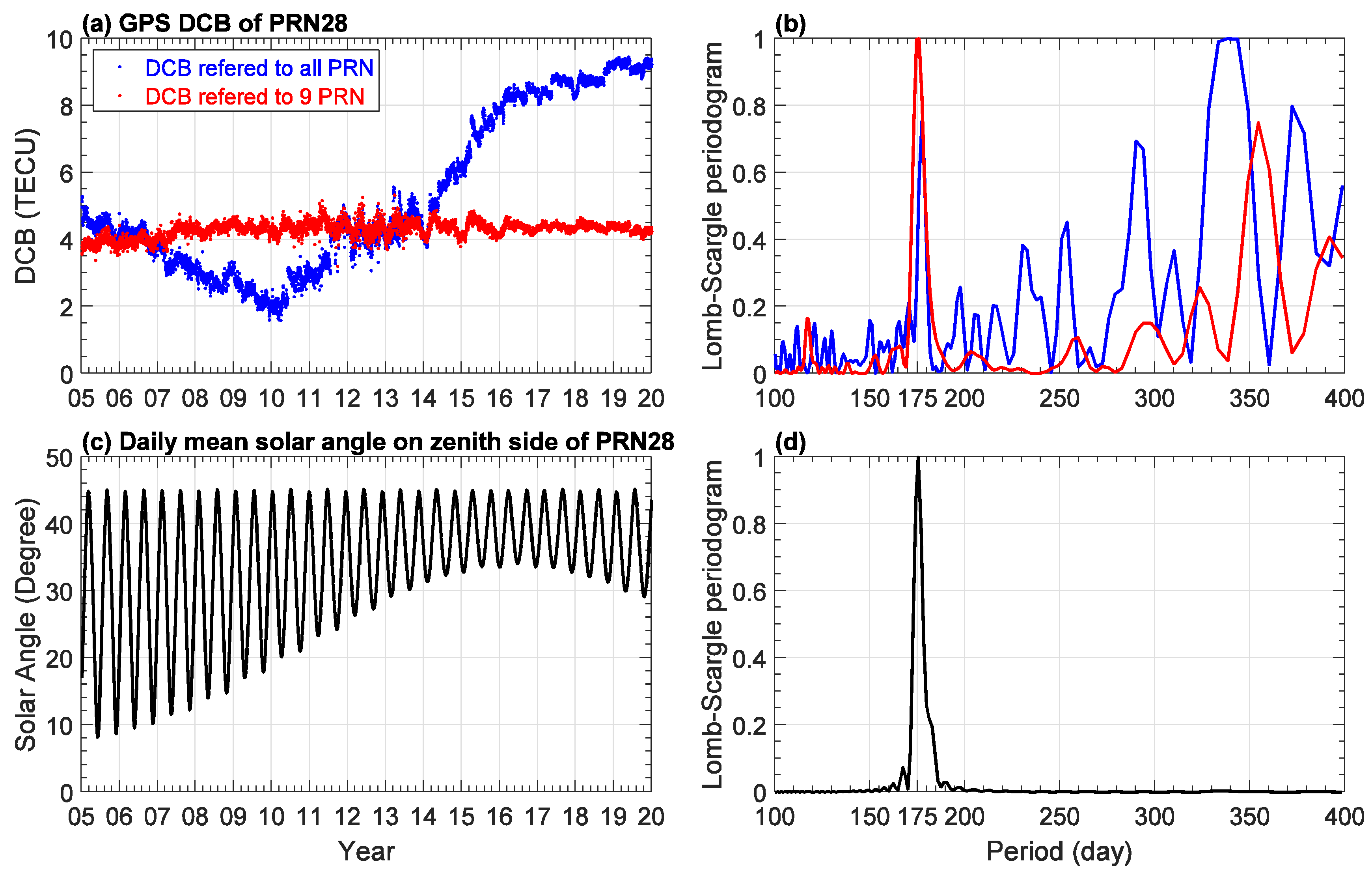
The reconstructed GPS DCB of PRN28 is shown in Figure 3a as an example. On the long-term scale, the reconstructed GPS DCB only showed a slight variation of less than 1 TECU. In addition, the reconstructed GPS DCB presented short-term periodic variations, which is less than one year. The Lomb–Scargle periodograms of the original and reconstructed GPS DCBs are shown in Figure 3b. It is clear that the original GPS DCB presented multiple periodic components, while some periodic components in the reconstructed GPS DCB became much weaker. This indicates that DCB reconstruction could filter out the artificial periodic variations. In addition, it is interesting that there is a prominent periodic component of about 175 days in Figure 3b, which is a little shorter than half of a sidereal year (182.625 days). Zhong et al. [3] demonstrated that the periodic variation of CHAMP satellite receiver DCB is mainly attributed to its hardware thermal status. Here, we calculated the daily mean solar angle on the zenith side of the GPS satellite to represent its hardware thermal status, as shown in Figure 3c. The periodogram of the daily mean solar angle in Figure 3d displayed a clear periodic component of about 175 days, which is generally in agreement with that of the GPS DCB. This period is matched with the period of a GPS draconitic year, which is equal to about 351.5 days. The GPS draconitic year is the time taken for the Sun to complete one revolution (return to the same point in space) with respect to the GPS orbital nodes, as seen from the Earth [7,8]. In one GPS draconitic year, there are exactly two eclipsing periods, which means that after 175.75 days, the elevation of the Sun above the orbital plane is the same, and the direction of the relative change in the height of the Sun is also the same. As a result of the Sun illumination and attitude of GPS satellites [9], every 175.75 days the Sun illuminates the same parts (electron circuits) of the GPS satellite in the same manner, which may change the hardware thermal status with the same period and further affect the DCB values. The periodic component of about 175 days can be seen in DCB around half of the total GPS satellites (not shown), but it is still not clear whether the effect of hardware thermal status on DCB is consistent for different GPS satellite block series. Many other GNSS-derived parameters are characterized by the draconitic repeatabilities or their harmonics, such as GNSS-based Earth Rotation Parameters [10]. Overall, both the solar-cycle-like and semiannual-like variations of the GPS DCB are artificial and not caused by the ionospheric variability.

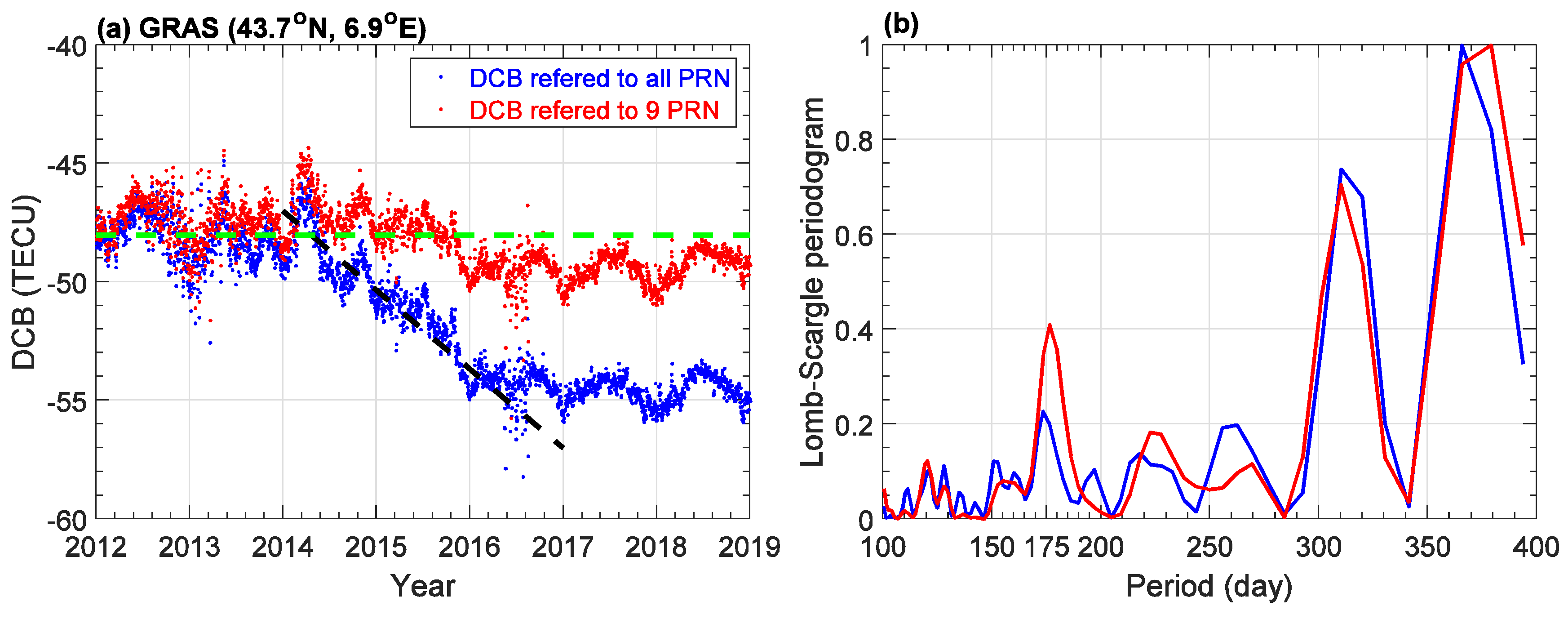
Figure 4 shows the original and reconstructed receiver DCBs for station GRAS as an example, as used in Choi et al. [1]. Again, the original receiver DCB presented a declined trend from 2014 to 2016, when F10.7 was mainly decreasing. However, the reconstructed receiver DCB only changed slightly during 2012–2017. The periodograms showed that the receiver DCB also presents a significant periodic component of about 176 days, which should be associated with the GPS draconitic year, as discussed above. In addition, there is a significant annual periodic component (365 days). The short-term variations of the receiver DCB are attributed to various factors, such as the hardware temperature [11]. From the comparison between surface temperature and the reconstructed receiver DCBs from many IGS stations (not shown), it illustrated that when the surface temperature reached its maximum (minimum), some of the reconstructed receiver DCBs also presented the maximum (minimum) values. Thus, the annual periodic component could probably be associated with the variations of the surface temperature. However, the manufacturer and model, antenna mounting position, cable construction, and thermal control could be complicated and different for each receiver, so it is difficult to draw a unified conclusion in respect of short-term variations of the receiver DCB.

As discussed above, both the long-term and short-term variations of the GPS DCBs and receiver DCBs are accessed. Though during specific periods, they were similar to the ionospheric variations by coincidence, they are not caused by the ionospheric variability physically. In the ionospheric TEC/DCB estimation, it is generally assumed that the ionosphere satisfies the spherically symmetric hypothesis or spherical harmonic expansion distribution. When the actual ionospheric distributions deviate from the assumption, the TEC measurement used in the DCB determination is subject to a large number of small random errors, and the probability distribution for the total statistical error is driven toward the Gaussian distribution, indicated by higher RMS (lower stability) for DCB. In TEC/DCB estimation, the larger the ionospheric TEC is, the greater the deviation from the spherically symmetric assumption would be, thus causing higher RMS (lower stability) for DCB, as presented by Choi et al. [1]. However, as mentioned above, in the physical sense the ionospheric TEC cannot alter the rDCB, which is essentially subject to the receiver hardware.

In summary, Choi et al. [1] concluded arbitrarily that the long-term variations of the receiver DCB are caused by the ionospheric variability on the basis of the problematic method. They were not aware of the effect of the GPS satellite replacement on the DCB determination. Overall, the study of Choi et al. [1] could introduce confusion and be misleading for the GNSS and the ionospheric communities.