Abstract
Recent advancements in environmental perception for autonomous vehicles have been driven by deep learning-based approaches. However, effective traffic target detection in complex environments remains a challenging task. This paper presents a novel dual-modal instance segmentation deep neural network (DM-ISDNN) by merging camera and LIDAR data, which can be used to deal with the problem of target detection in complex environments efficiently based on multi-sensor data fusion. Due to the sparseness of the LIDAR point cloud data, we propose a weight assignment function that assigns different weight coefficients to different feature pyramid convolutional layers for the LIDAR sub-network. We compare and analyze the adaptations of early-, middle-, and late-stage fusion architectures in depth. By comprehensively considering the detection accuracy and detection speed, the middle-stage fusion architecture with a weight assignment mechanism, with the best performance, is selected. This work has great significance for exploring the best feature fusion scheme of a multi-modal neural network. In addition, we apply a mask distribution function to improve the quality of the predicted mask. A dual-modal traffic object instance segmentation dataset is established using a 7481 camera and LIDAR data pairs from the KITTI dataset, with 79,118 manually annotated instance masks. To the best of our knowledge, there is no existing instance annotation for the KITTI dataset with such quality and volume. A novel dual-modal dataset, composed of 14,652 camera and LIDAR data pairs, is collected using our own developed autonomous vehicle under different environmental conditions in real driving scenarios, for which a total of 62,579 instance masks are obtained using semi-automatic annotation method. This dataset can be used to validate the detection performance under complex environmental conditions of instance segmentation networks. Experimental results on the dual-modal KITTI Benchmark demonstrate that DM-ISDNN using middle-stage data fusion and the weight assignment mechanism has better detection performance than single- and dual-modal networks with other data fusion strategies, which validates the robustness and effectiveness of the proposed method. Meanwhile, compared to the state-of-the-art instance segmentation networks, our method shows much better detection performance, in terms of AP and F1 score, on the dual-modal dataset collected under complex environmental conditions, which further validates the superiority of our method.
1. Introduction
With an increase in vehicle ownership, frequent traffic accidents, low vehicle traffic efficiency, and environmental pollution have become key factors restricting the development of the automotive industry [1]. Autonomous vehicles have been receiving attention due to their great potential for improving vehicle safety and performance, traffic efficiency, and energy efficiency [2]. An autonomous vehicle acquires information about the surrounding environment through environment-sensing sensors. However, robust and accurate detection, classification, and tracking of traffic targets, such as pedestrians, cyclists, vehicles, and so on, in complex environments remain a technical challenge for the sensing system of autonomous vehicles.
Southeast University independently developed an unmanned autonomous vehicle, which encountered many complicated environmental conditions during the usual experimental data collection process, as shown in Figure 1a–d.
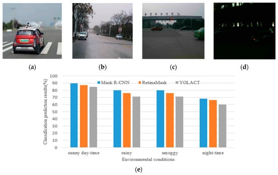
Figure 1.
Examples of complex environmental conditions: (a) sunny day-time (high illumination and great visibility); (b) rainy (low illumination); (c) smoggy (bad visibility); (d) night-time (low illumination and bad visibility); and (e) the average precision of classification prediction of Mask R-CNN, Retina-Mask, and YOLACT under different environmental conditions.
We tested Mask R-CNN [3], Retina-Mask [4], and YOLACT [5], which are state-of-the-art instance segmentation networks, on our own collected dataset under various environmental conditions (sunny day-time, rainy, smoggy, and night-time). The results indicated that the average classification prediction accuracy of ten classes of traffic objects (pedestrian, cyclist, cars, truck, traffic sign, traffic light, van, bus, train, and motorcyclist) decrease, to varying degrees, under the conditions of insufficient lighting and visibility by only using camera data. Therefore, multi-sensor data fusion-based target instance segmentation schemes must receive more and more attention. Commonly used on-board sensors include color cameras, infrared cameras, ultrasonic sensors, millimeter-wave radar, and laser LIDAR. At present, research on the detection of traffic targets for autonomous vehicles is mainly based on feature information of RGB images and depth information of traffic targets. Imran et al. combined an RGB image with a depth image collected by a Kinect camera and trained a convolution network with the four-channel flow for human activity recognition based on individual vision cues [6]. Silberman and Fergus presented an approach for indoor semantic segmentation by interpreting the major surfaces, targets, and support relations of an indoor scene from an RGB-D image [7]. A method for detecting a vehicle in a night driving scene taken from a vehicle monocular camera has been proposed by using a method called Center Surround Extremas to detect the blobs at high speed, based on the Laplacian of the Gaussian operator [8]. Cheon et al. proposed a vision-based vehicle detection system using the histogram of oriented gradients method, which is composed of a hypothesis generation step and a hypothesis verification step [9]. Aycard et al. proposed a complete perception fusion architecture based on the evidential framework, in order to detect and track moving targets by using an on-board sensing system composed of LIDAR and camera [10]. Gupta et al. studied the target detection problem of RGB-D images by using the semantic depth features of images and proposed a heterogeneous neural network combining two convolutional neural networks [11]. Eitel et al. built a novel Convolutional Neural Networks architecture composed of two separate CNN processing streams, in order to process RGB-D data for robust target recognition [12]. Wang et al. designed a novel neural network structure consisting of two convolutional neural networks (CNN), each of which extracts features and predicts saliency maps based on RGB or depth modes, and proposed an adaptive fusion scheme of saliency predictions for salient target detection [13]. Although these target detection methods have displayed great performance in the literature, RGB-D based methods usually work with depth cameras such as binocular cameras, Kinect cameras, or TOF cameras. However, these hardware devices are designed for close-range scenes (e.g., indoor environments). Such insufficient depth information leads to target detection methods based on RGB-D images rarely achieving satisfactory results, in terms of accuracy, efficiency, and timeliness, for autonomous vehicles in outdoor traffic scenarios.
Different sensors have their own advantages and limitations for traffic scene target detection. Cameras are sensitive to environmental conditions such as light and weather, and their detection accuracy relies heavily on complex image processing algorithms and high-performance image processors. Multi-line LIDAR provides real-time point cloud data that produces highly accurate 3D maps with high immunity to interference and are unaffected by light changes. However, laser LIDARs are relatively expensive and susceptible to severe weather conditions (e.g., rain or snow). The current research and application trend of target detection is to compensate for the defects of individual sensors through the information fusion of camera and LIDAR sensors, in order to improve the safety and reliability of the entire intelligent driving system. Premebida et al. proposed a context-based camera and LIDAR multi-sensor system for pedestrian detection in urban environments [14,15]. Zhang et al. presented a LIDAR and camera data fusion-based vehicle detection method which has two components: a hypothesis generation phase to generate positions that represent potential vehicles and a hypothesis verification phase to classify the corresponding targets [16]. Niessner et al. investigated three classifier training approaches to study the potential of Convolutional Neural Networks for vehicle classification based on RGB and LIDAR data [17]. Schlosser et al. explored various aspects of fusing LIDAR and color imagery for pedestrian detection based on convolutional neural networks, in which the LIDAR point clouds were up-sampled to dense depth maps and used as extra input channels [18]. Xiao et al. proposed a hybrid conditional random field to fuse the information from camera and LIDAR data for road detection [19]. Maalej et al. presented a multimodal scheme for target detection, recognition, and mapping based on the fusion of stereo camera frames, point cloud Velodyne LIDAR scans, and Vehicle-to-Vehicle technology [20].
Camera and LIDAR data fusion-based target detection methods are very efficient and suitable for practical applications in autonomous vehicles. Deep learning methods have been widely applied in the field of traffic target detection. This is mainly due to the deep convolutional neural network model, which can carry out supervised learning on labeled datasets and automatically extract feature information to obtain accurate classification results. In our work, we combine the two methods of deep learning and data fusion to detect, classify, and segment traffic targets. In such a way, the advantages of both methods can be inherited. First, sparse depth maps are captured by rotating LIDAR laser-point cloud data to the RGB image plane using a calibration matrix [21]. Then, the sparse LIDAR point cloud images are transformed into dense spherical depth images, which are used as the extra input channel in the deep neural networks to improve detection accuracy. Ten different traffic targets (car, bus, van, truck, train, pedestrian, cyclist, motorcyclist, traffic sign, and traffic light) are extracted by considering the ground truth from the KITTI dataset [22]. In our work, a high-quality manually annotated dataset of traffic targets is built using RGB images and LIDAR data from the KITTI dataset for network training and validation. We present a novel dual-modal instance segmentation network structure, which has four main components—a feature extraction sub-network, a data fusion sub-network, a classification sub-network, and a mask prediction sub-network—for data fusion and traffic target detection. In addition, considering the sparseness of LIDAR data, a weight assignment function of LIDAR data feature maps is designed to improve the detection accuracy. Finally, the proposed network is trained and tested using the manually annotated KITTI dataset and our own collected dataset. The detection results of the sensing system are provided to the driving cognitive module for vehicle decision-making and control in autonomous driving scenarios.
The main generalities and significances of this paper are:
- (1)
- A novel dual-modal instance segmentation deep neural network (DM-ISDNN) is presented for target detection by using a fused camera and LIDAR data. The proposed method provides significant technical contributions, which can be used for target detection under various complex environmental conditions (e.g., low illumination or bad visibility);
- (2)
- The early-, middle-, and late-stage data fusion architectures are compared and analyzed in-depth and the middle-stage fusion architecture with weight assignment mechanism has been selected for feature fusion in our paper by comprehensively considering the detection accuracy and detection speed. This work has great significance for exploring the best feature fusion scheme of a multi-modal neural network.
- (3)
- Due to the sparseness of LIDAR point cloud data, we propose a weight assignment function that assigns different weight coefficients to different feature pyramid convolutional layers for the LIDAR sub-network. A weight assignment mechanism is a novel exploration for optimizing the multi-sensor data feature fusion effect in deep neural networks. In addition, we apply a mask distribution function to improve the quality of the predicted mask;
- (4)
- We provide a manually annotated dual-modal traffic object instance segmentation dataset using a 7481 camera and LIDAR data pairs from the KITTI dataset, with 79,118 instance masks annotated. To the best of our knowledge, there is no existing instance annotation on the KITTI dataset with such quality and volume;
- (5)
- A novel dual-modal dataset with 14,652 camera and LIDAR data pairs is acquired using our own designed autonomous vehicle under different environmental conditions in real traffic scenarios. A total of 62,579 instance masks are obtained using the semi-automatic annotation method, which can be used to validate the effectiveness and efficiency of the instance segmentation deep neural networks under complex environmental conditions.
The rest of this paper is organized as follows: Section 2 describes the methodology of the proposed algorithm, including input LIDAR data preparation and network architecture description. Section 3 presents a description of the dataset and the network training method. Section 4 presents the experimental results, including a description of the autonomous vehicle perception system, experimental setup, analysis of the experimental results, and a comparison of classification results. Section 5 concludes the paper.
2. Methodology
2.1. Input LIDAR Data Preparation
The obtained 3D LIDAR point clouds can be projected onto the 2D image plane, such that they can be processed by the convolutional layer to obtain the feature information of the LIDAR data. In this work, a spherical map is obtained by projecting each 3D point onto a sphere, characterized by azimuth and zenith angles. It has the advantages of representing each 3D point in a dense and compact way, making it suitable for feature extraction. Figure 2a shows an example of an RGB image and a sparse LIDAR point cloud (bird’s-eye view) from the KITTI dataset.
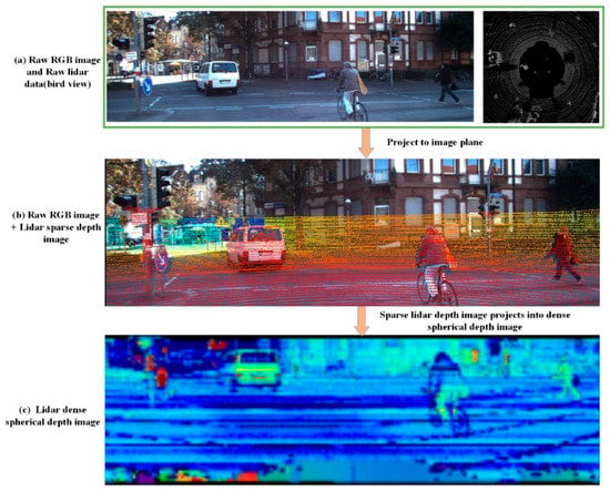
Figure 2.
Example of an RGB image and LIDAR data from KITTI dataset: (a) Raw RGB image and raw LIDAR point cloud data in bird’s-eye view; (b) sparse LIDAR depth image; and (c) dense LIDAR spherical depth image.
In the KITTI dataset, the LIDAR point clouds were captured by a Velodyne64E LIDAR sensor. Like other range scan data, LIDAR point cloud data can be projected and discretized into a 2D point map. It should be noted that the observation angle of the LIDAR and the camera are different; the view angle of the RGB images in the KITTI dataset is . Thus, only the LIDAR points which are located within the view field of the camera should be used for the projection. The projection function [23] used in this paper can be described as follows:
where are the Cartesian coordinates of the LIDAR points; and are the azimuth and zenith angles when observing the point, respectively; and are the average horizontal and vertical angle resolution between consecutive beam emitters, respectively; and r and c are the 2D map position indices on the projected image. The sparse-depth map obtained by projecting point cloud data to the image plane can be seen in Figure 2b.
We fill the element at in the 2D point map with 2-channel data , where . Note that and are coupled (as ) for rotation invariance around . Some points may be projected into the same 2D position, in which case the point nearer to the observer is kept. Elements in 2D positions where no 3D points are projected into are filled with . A dense LIDAR image can be obtained by up-sampling using bilateral filtering [23]. An example of the channel of the 2D dense spherical depth image is shown in Figure 2c. After the transformation, the image-type LIDAR data and RGB images are fed directly into the proposed network model.
2.2. Network Architecture
In order to achieve satisfactory efficiency, we build a novel dual-modal instance segmentation deep neural network (DM-ISDNN), following the architectures of the RetinaNet [24] and Mask R-CNN networks. Figure 3 shows a high-level overview of the proposed network architecture.
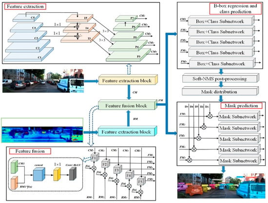
Figure 3.
Network architecture of our proposed traffic target instance segmentation model.
From Figure 3, we can see that the entire network has four basic sub-networks, which are a feature extraction sub-network, a data fusion sub-network, a classification sub-network, and a mask prediction sub-network. The inputs of the network model are RGB–LIDAR image pairs and the outputs are classification results with confidence, b-box localization, and mask proposals.
2.2.1. Feature Extraction Sub-Network
ResNet-101 was selected as the backbone model for the feature extraction sub-network, due to its superior feature extraction performance and a lower amount of parameters. The CNN layers, , are used for bottom-up feature extraction. The dimensionality of each CNN layer’s output is 64, 256, 512, 1024, and 2048, respectively. The intermediate convolution layers, , which are obtained by 1 × 1 convolution and 2× down-sampling operations, are used to eliminate aliasing effects between different convolutional layers and share a 3 × 3 convolution kernel. The FPN layers,, which are also obtained by 1 × 1 convolution and top-down connection operations, are used for fusing the multi-scale information of different convolutional layers. Following the FPN settings in [24], the dimensionality of each Feature Pyramid layer was set to 256. The convolution kernels had sizes of 3 × 3 and 1 × 1. The symbols and represent the extracted feature information of the RGB images and the dense LIDAR spherical depth images, respectively.
2.2.2. Data Fusion Sub-Network
The feature information of multi-sensor data extracted by deep convolutional neural networks can be fused using early-, middle-, and late-stage data fusion methods, as shown in Figure 4. Each fusion strategy has its own advantages and disadvantages [25]. Early-stage fusion refers to the fusion of raw or pre-processed data. However, neural network models trained in this way lack scalability; this means that, when the data category of the input channel changed, the model needs to be completely retrained. Late-stage fusion has a high degree of flexibility and scalability. However, this fusion method discards a large amount of feature information of the original and intermediate data, which may have a large impact on the final result of the entire network. Middle-stage data fusion makes full use of the advantages of early- and late-stage data fusion methods and, to some extent, circumvents the shortcomings of these two methods. In general, the lower convolutional layers contain more visual details, while higher convolutional layers contain more semantic information. Liu Y et al. [26] and Chen X et al. [27] designed several different convolutional network fusion architectures by integrating two-branch convolutional networks at different deep neural network stages. Their experiments showed that the middle stage with middle-level convolutional features had the best detection performance. This paper adopts the strategy of middle stage data fusion method. Furthermore, two middle stage data fusion strategies are considered to the fused camera and LIDAR data in our work. The features extracted by ResNet101 networks and FPN networks are fused, respectively, which is the main difference between these two data fusion strategies. The second middle stage data fusion strategy has better detection performance, according to the comparison of the experimental results in Section 4. Therefore, we adopt the weight assignment mechanism on the second middle stage data fusion model.
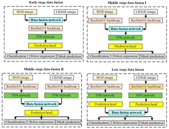
Figure 4.
Comparison of different data fusion strategies.
Considering the sparseness of LIDAR point cloud data, the number of LIDAR points distributed on a target decreases as the distance increases and, so, the feature information in the converted LIDAR images decreases. This phenomenon is disadvantageous for target detection using RGB and LIDAR images. Although some algorithms have used multi-scale feature fusion to improve the detection accuracy, they generally used the fused features for prediction. The difference when using FPN is that prediction is performed independently at different feature layers [28]. Most target detection algorithms use only top-level features for prediction, whereas we know that lower-level features have less semantic information—although the target position is more accurate, which is more suitable for the detection of small targets. On the other hand, high-level convolutional layers contain richer semantic information but rougher target position, which is more suitable for large target detection [29]. Like RetinaNet, our network does not produce P0, P1, and P2 layers. The size of the square anchors in the P3 layer is 24 pixels and the anchor size of subsequent layers are twice the size of the previous one—that is, [48,96,192,384], with aspect ratios [2:1,1:1,1:2]—which means it is easier to detect a larger target using the P7 layer. Therefore, we first multiply the LIDAR feature map by a coefficient and then perform data fusion, as shown in Figure 5.
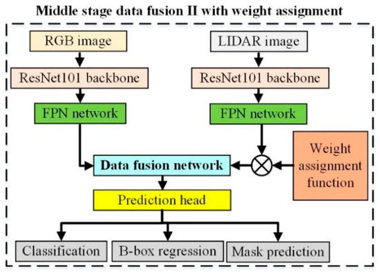
Figure 5.
Middle-stage data fusion II with weight assignment.
The expression of the weight assignment function can be written as:
where num represents the number of the feature map to be fused (see Figure 3) and is the corresponding feature impact factor.
The feature information extracted by the feature extraction sub-network is fused by the fusion layers . Each fusion block includes similar feature map concatenation, 1 × 1 convolutional, and ReLU convolutional layers, as shown in Figure 3. The feature maps from the two modalities are concatenated and a 1 × 1 convolutional layer is then performed on the concatenated feature maps, in order to reduce the dimension and linearly merge the dual-modal features. The parameters of the convolution kernel in the 1 × 1 convolutional layer are trained as well. Then, the fused feature maps are processed by the same operation as in a single-modal detection network.
2.2.3. Bounding Box Prediction and Classification Sub-Network
In this work, the outputs of the fusion feature layers are used for bounding box and class predictions. The bounding box prediction and classification sub-network performs a fully convolution-like operation on the output of each fusion layer to predict the probability values of the K categories for each anchor at each spatial location. The specific operation is that four 3 × 3 × C convolutional layers are designed for each fusion layer, where each of them is connected to a ReLU layer (the symbol C represents the dimensionality of each fusion layer). Finally, an output 3 × 3 × K × A convolutional layer with point-wise sigmoid non-linearities is used to produce K × A binary predictions for each spatial location, where A is the number of anchors. In this work, the values of A, C, and K are set to 9, 256, and 10, respectively. For bounding box regression, four linear outputs are used to predict the relative offset of each anchor and the ground truth box of anchors at each spatial location. The bounding box regression with a class-agnostic setting is used to significantly reduce the number of parameters.
2.2.4. Mask Prediction Sub-Network
For mask prediction, we apply the soft non-maximum suppression (Soft-NMS) [28] detector after bounding box prediction, in order to duplicate prediction boxes and extract the top N scored bounding box predictions as mask proposals (where N is variable). These mask proposals are then distributed to sample features from the appropriate fusion layers , according to the following mask distribution function:
where and are the width and height of the detection region, and are the width and height of resized input image (in order to keep the evaluation time of each image basically the same, we do not retain the aspect ratio of the original image, but uniformly resize the size of image to ), and represents the ratio of the detected region to the total image area. If the ratio is less than 0.2, it will be assigned to the feature layer ; between 0.2 and 0.4, it is assigned to ; between 0.4 and 0.6, it is assigned to ; between 0.6 and 0.8, it is assigned to ; and if the ratio is larger than 0.8, it is assigned to .
2.2.5. Loss Function
The proposed traffic target instance segmentation network is trained by minimizing the following joint loss function:
where is the detection loss defined over the final detections, is the classification prediction loss, is the b-box regression loss, is the image-level per-pixel loss, and , , and are corresponding weight coefficients.
Let and respectively represent the ground-truth and predicted classification. The classification prediction loss can be obtained as:
where is the number of detection regions and is the multi-class classification cross-entropy loss function.
Let and respectively represent the ground-truth and predicted b-box. The b-box regression loss can be obtained as:
where the is the number of feature maps and is the smooth-L1 loss function for b-box regression. The parameter settings of the classification and b-box regression loss functions follow those of the single-shot multi-box detector [30].
Let and respectively represent the ground-truth and predicted segmentation masks. The image-level per-pixel loss can be written as:
where is the number of the feature maps at the pixel level and is the segmentation cross-entropy loss function.
3. Dataset and Network Training
3.1. Dual-Modal KITTI Dataset
We trained the proposed DM-ISDNN using RGB images and 3D point cloud data from the dual-modal KITTI dataset to validate the effectiveness of the proposed method. The sparse LIDAR point clouds were transformed into dense spherical depth images. The training dataset contained 5000 RGB and LIDAR image pairs and 52,886 labeled traffic targets were annotated. The validation image dataset contained 2481 RGB and LIDAR image pairs and 26,232 labeled traffic targets were annotated. Training and validation image pair examples can be seen in Figure 6. The datasets included ten traffic target categories: pedestrians, cyclists, trains, cars, buses, trucks, vans, motorcyclists, traffic lights, and traffic signs. The resolutions of the RGB and LIDAR images were normalized to 1392 × 512 pixels.

Figure 6.
RGB–LIDAR image pair examples in training and validation datasets: (a) pedestrian; (b) cyclist; (c) cars; (d) truck; (e) traffic sign; (f) traffic light; (g) van; (h) bus; (i) train; and (j) motorcyclist.
The training and validation datasets contained a total of 79,118 labeled traffic targets. We built the instance segmentation dual-modal dataset using the urban road subset of the KITTI dataset. Therefore, the number of cars was larger than other categories, followed by pedestrians, traffic signs, and traffic lights, while the number of trains and motorcyclists were the smallest. This distribution is consistent with our daily traffic situation. Most traffic targets encountered by autonomous vehicles on urban roads are cars, pedestrians, traffic lights, and traffic signs.
3.2. Dual-Modal Zhi-Shan Dataset
3.2.1. Data Collection Platform
The images in the KITTI dataset were basically obtained under clear weather conditions. Therefore, in order to verify the detection performance of the proposed method under complex conditions (e.g., low illumination), we collected and annotated our own dataset, which we named the dual-modal Zhi-Shan dataset. The autonomous vehicle Zhi-Shan, which was designed and developed by Southeast University, was used for camera and LIDAR data collection. The overall appearance and sensing system installation distribution of the autonomous vehicle are shown in Figure 7.
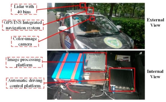
Figure 7.
Sensing system of the Zhi-Shan autonomous driving vehicle.
The sensing system consisted of a 40-line laser LIDAR, a millimeter-wave radar, a GPS/INS integrated navigation system, a camera, an automatic driving control platform, and an NVIDIA JTX 2 image processing platform. A detailed description of the sensing system is provided in Table 1.

Table 1.
Configuration of the Zhi-Shan intelligent vehicle.
3.2.2. Distribution of the Dual-Modal Zhi-Shan Dataset
We collected 14,652 camera and LIDAR data pairs in different environmental conditions and time periods for testing the network detection performance and for comparison with state-of-the-art instance segmentation networks, as shown in Table 2. A total of 62579 instance masks were obtained using a semi-automatic annotation method. In order to produce high-quality annotation results with less manpower, we used a semi-automatic annotation method to generate instance masks for the dual-modal Zhi-Shan dataset. The proposed model, DM-ISDNN using middle-stage data fusion and the weight assignment mechanism, was used to automatically generate instance masks, following which we used manual annotation to further modify and improve the quality of dataset annotations. Our labelling method can automatically segment all objects and we only needed to focus on improving the annotation results in complex driving scenarios.

Table 2.
Distribution of the dual-modal Zhi-Shan dataset.
3.3. Network Training
To train the proposed deep learning neural network in this paper, we followed the original settings of the ResNet-101-FPN backbone. The images were resized to make the shorter side equal to 550 pixels while limiting the larger side to 550 pixels. We used a batch size of 16 images, a weight decay of , a momentum of 0.9, and trained for 15,000 iterations with a base learning rate of 0.01, which was dropped to 0.001 and 0.0001 at iterations 5000 and 10,000, respectively.
4. Experiment and Analysis of Proposed Method
4.1. Experimental Setup
We used the manually annotated dual-modal traffic target dataset extracted from KITTI and the semi-automatically annotated dual-modal traffic target dataset captured with our own autonomous vehicle for network training and testing. We trained our network on servers with two NVIDIA GeForce GTX 1080TI GPUs. The training time was about 87 h. The on-board hardware platform was an NVIDIA Jetson TX2 with ARM A57 CPUs and one GPU. The two software development platforms were comprised of a convolutional architecture for fast feature embedding and NVIDIA CUDA 9.0. The operating system was Ubuntu 16.04.
4.2. Comparison of Experimental Results and Analysis
4.2.1. Average Precision
We employed the average precision (AP) at different intersection over union (IoU) thresholds (AP, AP50, AP75) as the metrics to evaluate the performance of instance segmentation. We only evaluated objects larger than 25 pixels in height, following the same principle as the KITTI object detection benchmark. The AP represents the quality of the model, which can be obtained as:
where is the precision, is the recall, TP represents the true positive samples, FP denotes the false-positive samples, TN represents the true negative samples, FN denotes the false-negative samples, and C is the number of categories.
The is another criterion used to evaluate the detection accuracy, which can be obtained by calculating the overlap ratio between predicted and true bounding boxes, as follows:
where is the intersection area of the predicted and true bounding boxes and denotes the union area of the predicted and true bounding boxes. AP50 and AP75 represent the AP values at and , respectively.
In this paper, we only compare the detection performance of mask prediction; the AP values for classification and bounding box regression had the same tendency, as shown in Table 3.

Table 3.
Comparison of detection performance using different data fusion strategies.
From the table, we can see that the dual-modal network using middle-stage fusion strategy II with weight assignment showed the highest average precision and the single-modal instance segmentation deep neural network (SM-ISDNN) with RGB images as input had the lowest scores. Therefore, we adopted the strategy of the second middle-stage data fusion method with weight assignment.
4.2.2. Processing Time
The processing time is a critical metric for autonomous vehicles. When the network cannot handle information in real-time, delays will accumulate and affect the whole autonomous driving system. Losing any key frame may influence subsequent control decisions, regardless of the object being a pedestrian or a car. We trained the whole network with 15,000 iterations and saved the trained model after every 1000 iterations. We randomly selected 1500 images from the validation image dataset to test the processing time performance. The frames per second (FPS) of the proposed network under different iterations considerably changed, reaching approximately 37 FPS using the RGB-based method and ranging between 29.5–35 FPS for the different data fusion strategies used in this work, as shown in Figure 8.
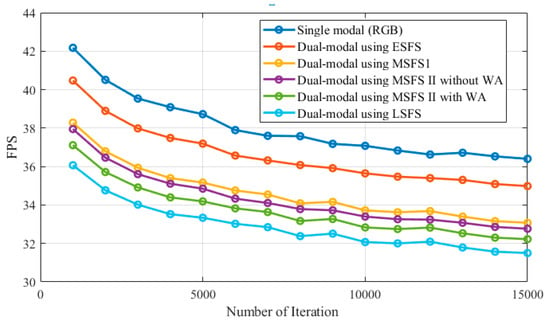
Figure 8.
Frames per second (FPS) of single- and dual-modal networks with different data fusion strategies.
Cameras recently used in autonomous vehicles feature a common standard of approximately 25 FPS. The only difference is that the camera has a much larger resolution than the input of our network, but this difference can be fixed by changing the scaling to the same resolution of . From the above analysis, we can see that our network model can essentially meet the real-time requirement of environmental perception for autonomous vehicles.
4.2.3. Average Accuracy
We compared the average accuracy of the proposed network using the F1 score metric under the two conditions by using the traditional RGB image with RGB–LIDAR image pairs. The F1 score is commonly used for evaluating the performance of neural networks and can be defined as follows:
where P is the precision and R is the recall.
Figure 9 shows the F1 score curves.
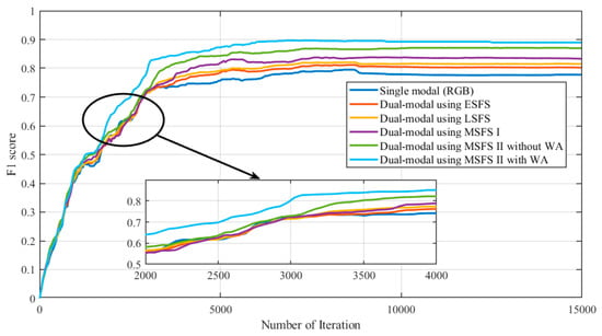
Figure 9.
F1 scores of RGB-based and RGB–LIDAR-based methods.
All curves showed similar tendencies, with average accuracy plateauing after approximately 5000 iterations. Using the proposed method, with an increase in the depth of information provided, the dual-modal RGB–LIDAR data led to higher accuracy than the pure RGB data for classification prediction. The RGB–LIDAR-based methods consistently presented better accuracies than the RGB-based method after 1000 training iterations.
4.2.4. Changes of Loss Functions
The average losses of combinations of datasets are shown in Figure 10a–c. The average loss continuously dropped as the number of iterations increased. DM-ISDNN consistently converged more rapidly than SM-ISDNN.
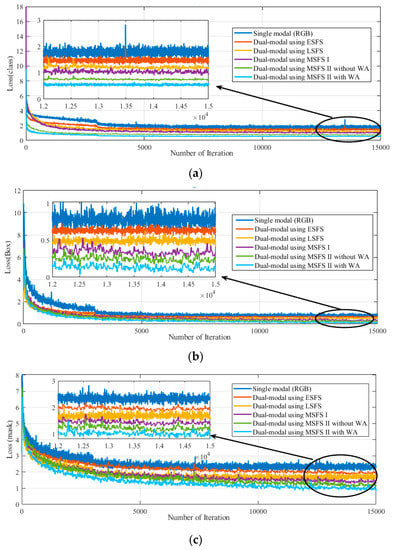
Figure 10.
Loss curves of RGB-based and RGB–Lidar-based methods: (a) classification loss; (b) b-box regression loss; and (c) mask loss.
4.2.5. Classification Prediction Results
We also calculated the confusion matrices for validation data using SM-ISDNN and DM-ISDNN, which are shown in Figure 11. The values in the main diagonal are the correctly classified items and the numbers are the percentages of precision for each category of traffic objects, which is commonly used to evaluate the performance of object detection networks and can be defined as the fraction of relevant instances among all retrieved instances. For example, considering traffic lights, there were 1016 annotations in the validation dataset. The number of traffic light instances that were relevant and which were correctly identified as relevant by SM-ISDNN and DM-ISDNN were 941 and 950, respectively. Therefore, their respective precision values for traffic lights were 92.6% and 93.5%. The rest were the misclassified items. From the classification prediction results, we can see that, even if only color images were used, good detection results were obtained. This is mainly because the KITTI dataset was acquired under great environmental conditions, with image quality and image resolution both being high. However, in complex environments (e.g., low illumination and low visibility), the detection accuracy cannot be guaranteed when only using the color images, as discussed in detail in the following sections.
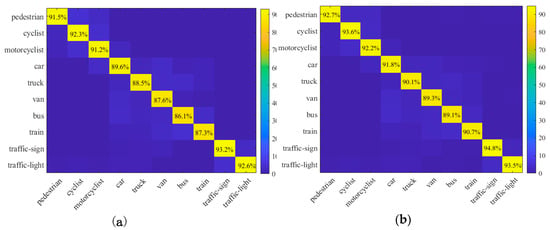
Figure 11.
Confusion matrices for validation data: (a) Single-modal network; and (b) Dual-modal network using Middle-stage fusion strategy (MSFS) II with weight assignment (WA).
From Figure 11, we can see that the main error happened when road traffic participants were classified as other types of road traffic participants (i.e., “pedestrian”, “cyclist”, and “motorcyclist”) and when vehicles were classified as other types of vehicles (i.e., “car”, “truck”, “van”, “bus”, and “train”). The reason for this could be that these road traffic participants are very similar in appearance in the current dataset and their backgrounds are also very similar. The misclassification of vehicles may be due to similar reasons. In addition, the precision of classification prediction of the dual-modal network using the middle-stage fusion strategy (MSFS) II with weight assignment (WA)-based method was higher than that of the single-modal network-based method. This shows that increasing the feature information by using LIDAR images is conducive to better classification of traffic targets.
4.3. Influence of the Feature Impact Factor
The weight assignment function includes a key parameter, the feature impact factor a, which represents the dependence of our model on different FPN layers. The higher the value of the parameter, the less we rely on the low-level pyramid feature layers, which means that we prefer to use the high-level semantic information of LIDAR images to classify the target. In this paper, the influence of the feature impact factor a was tested by setting its value to 1.0, 0.6, 0.4, or 0.2. The training results are shown in Figure 12.
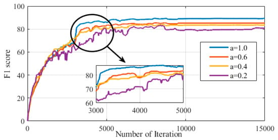
Figure 12.
Average classification prediction accuracies when using different values of the feature impact factor.
Based on the above results, we can see that the classification prediction accuracies were significantly higher when . Due to the sparseness of the radar point cloud data, it is not conducive to carry out small-target detection using LIDAR images and, so, using low-level feature layer information may lead to a reduction in the detection accuracy.
The loss function curves are shown in Figure 13.
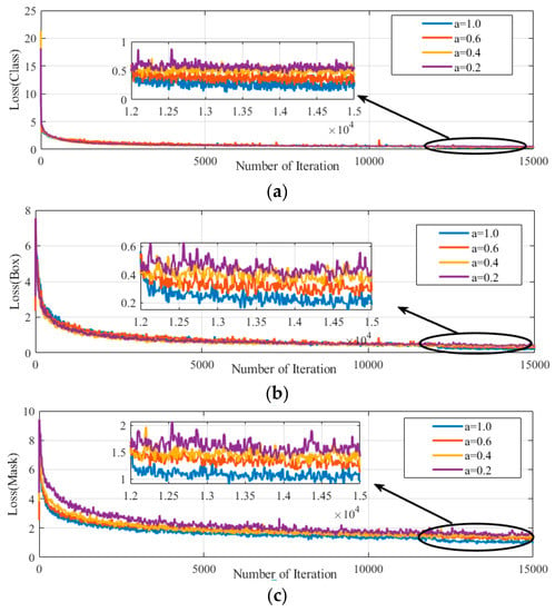
Figure 13.
Loss curves using different values of the feature impact factor: (a) classification loss; (b) b-box regression loss; and (c) mask loss.
We can see that lower loss could be obtained by using a higher value of the feature impact factor, indicating that the performance of the proposed model was better when using the high-level semantic information of LIDAR images. However, we do not believe that the performance will continue to increase with the value of this parameter, as, if its value is too high, too many image details will be ignored, which is obviously not beneficial for target detection and is not conducive for taking advantage of the FPN network.
5. Detection Results Comparison on The Dual-Modal Zhi-Shan Dataset
A comparison of the detection results obtained using Mask R-CNN, RetinaMask, YOLACT, and the proposed method is shown in Figure 14. It can be seen that, although RetinaMask and YOLACT have great detection performance in complex real traffic scenes, the proposed method had a higher detection accuracy. Mask R-CNN, as a classic two-stage detection method, had the best detection accuracy, but also had many false detections. In addition, we can see from Figure 14(a4–e4) that, in the absence of illumination, the traditional Mask R-CNN, RetinaMask, and YOLACT methods could not detect the traffic targets, while the proposed method still performed satisfactorily.
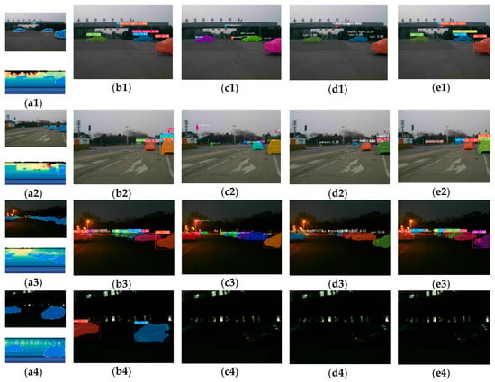
Figure 14.
Detection results with our own testing datasets: (a1–a4) raw RGB–LIDAR image pairs with ground truth; (b1–b4) detection results of the proposed method; (c1–c4) detection results of Mask R-CNN; (d1–d4) detection results of RetinaMask; and (e1–e4) detection results of YOLACT.
In order to further confirm the effectiveness of our proposed method, we compared the DM-ISDNN to state-of-the-art instance segmentation networks on our dataset. The results are shown in Table 4.

Table 4.
Comparison with state-of-the-art instance segmentation networks for FPS and mask AP.
The results were computed using two NVIDIA GeForce GTX 1080TI GPUs and, so, the FPS values listed in this table may differ from those in the original paper. In addition, we used ResNet-18-FPN, ResNet-50-FPN, and ResNet-101-FPN as backbone architectures, respectively, for the proposed DM-ISDNN. When ResNet-18-FPN was used as a backbone, the network had the highest calculation speed and the FPS reached 37.3, but the AP was the lowest. When ResNet-101-FPN was used as a backbone, at the 50% IoU threshold, our proposed model achieved 59.4 AP, while Mask R-CNN, Retina-Mask, and YOLACT networks achieved 58.0 AP, 55.4 AP, and 48.5 AP, respectively. This shows that our model can provide the highest quality mask. In addition, the FPS value achieved was 27, which meets the real-time requirements of autonomous vehicles.
Considering the above testing results, we can see that the proposed network is still robust in complex environmental conditions with a lack of illumination and visibility. Under dusk and night-time conditions, due to a serious lack of illumination, it is almost impossible to identify traffic targets in RGB images; however, the features of these traffic targets are still obvious in LIDAR images—see Figure 14(a3,a4). Therefore, we achieved satisfactory detection results by using a multi-sensor data fusion-based approach.
6. Conclusions
In this paper, we proposed a novel dual-modal instance segmentation network, which has great significance for dealing with the problem of target detection in complex environments efficiently based on multi-sensor data fusion. We first up-sampled LIDAR point clouds and converted the up-sampled data into pixel-level images. Then, we fed the RGB images, together with LIDAR images, into the proposed network to perform feature learning from raw input information, merging the feature maps in the middle stage and obtaining informative feature representation to classify targets and predict corresponding masks. The early-, middle-, and late-stage data fusion architectures are compared and analyzed in-depth, which has great significance for exploring the best feature fusion scheme of multi-modal neural networks. By comprehensively considering the detection accuracy and detection speed, the middle-stage fusion architecture with a weight assignment mechanism has been selected for feature fusion in our paper. The proposed approach, in which camera data are fused with LIDAR data, exhibited superior classification accuracy over the approach using only RGB images from the manually annotated dual-modal KITTI dataset. To the best of our knowledge, there is no existing instance annotation on the KITTI dataset with such quality and volume. In addition, by comparing the training and testing results, we observed that using high-level semantic information of LIDAR images could significantly improve detection accuracy. The camera and LIDAR in our own designed Zhi-Shan autonomous vehicle were used to collect images and point clouds to form a novel dual-modal dataset with semi-automatic annotation for validation of the detection performance of networks under complex environmental conditions. We trained and tested the proposed network using the manually annotated KITTI dataset and our own collected datasets with semi-automatic annotations. Our experimental results validated the effectiveness and efficiency of the proposed approach under complex environmental conditions, through the use of additional LIDAR data input and assigning appropriate weight coefficients to different feature layers. Compared to the state-of-the-art instance segmentation networks, our method demonstrated much better detection performance, in terms of AP and F1 score, on the dual-modal Zhi-Shan dataset collected under complex environmental conditions, which further validates the superiority of our method. It is worth noting that the dataset we collected only contained four weather conditions—”Sunny day-time”, “Rainy”, “Smoggy”, and “Night-time”—and that the images are quite different, in terms of illumination and atmospheric visibility. However, we did not consider other factors that may degrade image quality, such as blur and noise. In addition, our experimental results were all performed on a high-performance image processing server. Whether the proposed method can meet the detection accuracy and real-time requirements in the same timeframe on the vehicle-mounted processor with limited computation ability requires further verification. In our further work, we will continue to increase the scale and coverage of the dual-modal Zhi-Shan dataset. Furthermore, we will also perform experiments in more real, complicated traffic scenarios, in order to verify the ability of the proposed approach in classifying targets in an autonomous vehicle environment based on the vehicle-mounted domain controller. It should be noted that the main research significance of this paper is to explore a novel multi-modal instance segmentation neural network model with an optimal data fusion scheme. The proposed deep neural network model can not only be used for common traffic targets detection as mentioned in this paper, but also for solving some other similar problems, such as air–ground cooperative targets perception and vehicle–road cooperative targets perception, which will be further discussed in our future work.
Author Contributions
In this article, the author’s contributions are shown below: Methodology, K.G.; writing—original draft preparation, G.D.; project administration, G.Y.; data curation, J.H.; investigation, K.G.; resources, K.G. All authors have read and agreed to the published version of the manuscript.
Funding
National Natural Science Foundation of China (Grant No. 51905095) and National Natural Science Foundation of Jiangsu Province (Grant No. BK20180401).
Acknowledgments
We appreciate the critical and constructive comments and suggestion from the reviewers that helped improve the quality of this manuscript. We also would like to offer our sincere thanks to those who participated in the data processing and provided constructive comments for this study.
Conflicts of Interest
The authors declare no conflict of interest.
References
- Zhu, J.S.; Ke, S.; Sen, J.; Lin, W.D.; Hou, X.X.; Liu, B.Z.; Qiu, G.P. Bidirectional Long Short-Term Memory Network for Vehicle Behavior Recognition. Remote Sens. 2018, 10, 887. [Google Scholar] [CrossRef]
- Stateczny, A.; Kazimierski, W.; Gronska-Sledz, D.; Motyl, W. The Empirical Application of Automotive 3D Radar Sensor for Target Detection for an Autonomous Surface Vehicle’s Navigation. Remote Sens. 2019, 11, 1156. [Google Scholar] [CrossRef]
- Kaiming, H.; Georgia, G.; Piotr, D.; Girshick, R. Mask R-CNN. IEEE Trans. Pattern Anal. Mach. Intell. 2020, 42, 386–397. [Google Scholar]
- Fu, C.Y.; Shvets, M.; Berg, A.C. RetinaMask: Learning to Predict Masks Improves State-of-the-Art Single-Shot Detection for Free. Available online: https://arxiv.org/abs/1703.06870 (accessed on 13 September 2020).
- Bolya, D.; Zhou, C.; Xiao, F.; Lee, Y.J. YOLACT: Real-time Instance Segmentation. In Proceedings of the IEEE/CVF International Conference on Computer Vision, Seoul, Korea, 27 October–2 November 2019. [Google Scholar]
- Khaire, P.; Kumar, P.; Imran, J. Combining CNN streams of RGB-D and skeletal data for human activity recognition. Pattern Recognit. Lett. 2018, 115, 107–116. [Google Scholar] [CrossRef]
- Silberman, N.; Hoiem, D.; Kohli, P.; Fergus, R. Indoor segmentation and support inference from RGB-D images. In Proceedings of the European Conference on Computer Vision, Florence, Italy, 7–13 October 2012. [Google Scholar]
- Kosaka, N.; Ohashi, G. Vision-Based Nighttime Vehicle Detection Using CenSurE and SVM. IEEE Trans. Intell. Transp. Syst. 2015, 16, 1–10. [Google Scholar] [CrossRef]
- Cheon, M.; Lee, W.; Yoon, C.; Park, M. Vision-Based Vehicle Detection System With Consideration of the Detecting Location. IEEE Trans. Intell. Transp. Syst. 2012, 13, 1243–1252. [Google Scholar] [CrossRef]
- Chavez-Garcia, R.O.; Aycard, O. Multiple Sensor Fusion and Classification for Moving Target Detection and Tracking. IEEE Trans. Intell. Transp. Syst. 2015, 17, 1–10. [Google Scholar]
- Gupta, S.; Girshick, R.; Arbeláez, P. Learning Rich Features from RGB-D Images for Target Detection and Segmentation. Lect. Notes Comput. Sci. 2014, 8695, 345–360. [Google Scholar]
- Eitel, A.; Springenberg, J.T.; Spinello, L.; Riedmiller, M.; Burgard, W. Multimodal Deep Learning for Robust RGB-D Object Recognition. In Proceedings of the International Conference on Intelligent Robots and Systems, Daejeon, Korea, 28 September–2 October 2015. [Google Scholar]
- Song, H.; Choi, W.; Kim, H. Robust vision-based relative-localization approach using an RGB-depth camera and LiDAR sensor fusion. IEEE Trans. Ind. Electron. 2016, 63, 3725–3736. [Google Scholar] [CrossRef]
- He, W.; Li, Z.; Kai, Z.; Shi, Y.S.; Zhao, C.; Chen, X. Accurate and automatic extrinsic calibration method for blade measurement system integrated by different optical sensors. In Proceedings of the Optical Metrology & Inspection for Industrial Applications III, Beijing, China, 9–11 October 2014. [Google Scholar]
- Premebida, C.; Nunes, U. Fusing LIDAR, camera and semantic information: A context-based approach for pedestrian detection. Int. J. Rob. Res. 2013, 32, 371–384. [Google Scholar] [CrossRef]
- Zhang, F.; Clarke, D.; Knoll, A. Vehicle detection based on LIDAR and camera fusion. In Proceedings of the IEEE International Conference on Intelligent Transportation Systems, Qingdao, China, 8–11 October 2014. [Google Scholar]
- Niessner, R.; Schilling, H.; Jutzi, B. Investigations on the potential of convolutional neural networks for vehicle classification based on RGB and LIDAR data. Remote Sens. Space Inform. Sci. 2017, 4, 115–123. [Google Scholar] [CrossRef]
- Schlosser, J.; Chow, C.K.; Kira, Z. Fusing LIDAR and images for pedestrian detection using convolutional neural networks. In Proceedings of the IEEE International Conference on Robotics and Automation, Stockholm, Sweden, 16–21 May 2016. [Google Scholar]
- Xiao, L.; Wang, R.; Dai, B.; Fang, Y.Q.; Liu, D.X.; Wu, T. Hybrid conditional random field based camera-LIDAR fusion for road detection. Inf. Sci. 2018, 432, 543–558. [Google Scholar] [CrossRef]
- Almagambetov, A.; Velipasalar, S.; Casares, M. Robust and Computationally Lightweight Autonomous Tracking of Vehicle Taillights and Signal Detection by Embedded Smart Cameras. IEEE Trans. Ind. Electron. 2015, 62, 3732–3741. [Google Scholar] [CrossRef]
- Gneeniss, A.S.; Mills, J.P.; Miller, P.E. In-flight photogrammetric camera calibration and validation via complementary LIDAR. J. Photogramm. Remote Sens. 2015, 100, 3–13. [Google Scholar] [CrossRef]
- Geiger, A.; Lenz, P.; Stiller, C.; Urtasun, R. Vision meets robotics: The KITTI dataset Int. J. Rob. Res. 2013, 32, 1231–1237. [Google Scholar] [CrossRef]
- Premebida, C.; Carreira, J.; Batista, J.; Nunes, U. Pedestrian detection combining RGB and dense LIDAR data. In Proceedings of the IEEE/RSJ International Conference on Intelligent Robots and Systems, Chicago, IL, USA, 14–18 September 2014. [Google Scholar]
- Lin, T.Y.; Goyal, P.; Girshick, R.; He, K.; Dollar, P. Focal Loss for Dense Object Detection. IEEE Trans. Pattern Anal. Mach. Intell. 2020, 42, 318–327. [Google Scholar] [CrossRef] [PubMed]
- Feng, D.; Haase-Schuetz, C.; Rosenbaum, L.; Hertlein, H. Deep Multi-Modal Target Detection and Semantic Segmentation for Autonomous Driving: Datasets, Methods, and Challenges. Available online: https://arxiv.org/abs/1902.07830?context=cs (accessed on 8 September 2020).
- Sawaragi, T.; Kudoh, T. Self-reflective segmentation of human bodily motions using recurrent neural networks. IEEE Trans. Ind. Electron. 2013, 50, 903–911. [Google Scholar] [CrossRef]
- Chen, X.; Ma, H.; Wan, J.; Ma, H.; Wan, J.; Li, B. Multi-view 3d object detection network for autonomous driving. In Proceedings of the IEEE Conference on Computer Vision and Pattern Recognition, Honolulu, HI, USA, 21–26 July 2017. [Google Scholar]
- Lin, T.Y.; Dollár, P.; Girshick, R. Feature pyramid networks for target detection. In Proceedings of the IEEE Conference on Computer Vision and Pattern Recognition, Honolulu, HI, USA, 21–26 July 2017. [Google Scholar]
- Bodla, N.; Singh, B.; Chellappa, R. Soft-NMS—Improving Target. Detection with One Line of Code. In Proceedings of the IEEE International Conference on Computer Vision, Venice, Italy, 22–29 October 2017. [Google Scholar]
- Liu, W.; Anguelov, D.; Erhan, D. SSD: Single Shot MultiBox Detector. In Proceedings of the European Conference on Computer Vision, Amsterdam, The Netherlands, 8–14 September 2016. [Google Scholar]
© 2020 by the authors. Licensee MDPI, Basel, Switzerland. This article is an open access article distributed under the terms and conditions of the Creative Commons Attribution (CC BY) license (http://creativecommons.org/licenses/by/4.0/).