Deep Learning in Hyperspectral Image Reconstruction from Single RGB images—A Case Study on Tomato Quality Parameters

 ,
,  , , and
Abstract
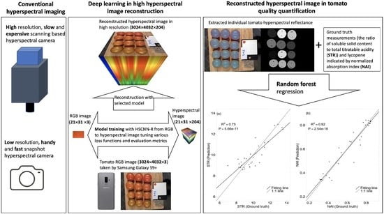
1. Introduction
2. Materials and Methods
2.1. Plant Material, Growth Conditions, and Tomato Sampling
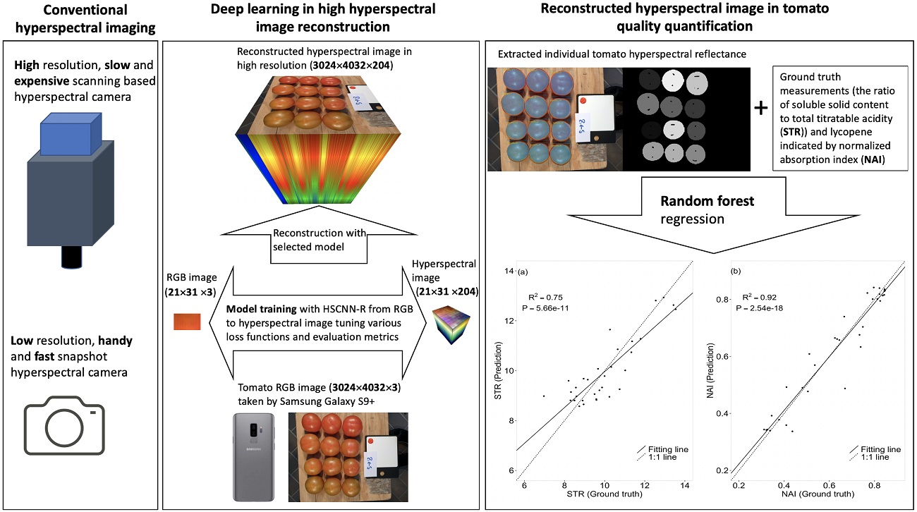
2.2. Image Acquisition
2.3. Tomato Quality Parameters (“Ground Truth”)
2.4. Model Selection, Training and Validation
2.5. Image Segmentation and Quality Parameter Prediction
3. Results
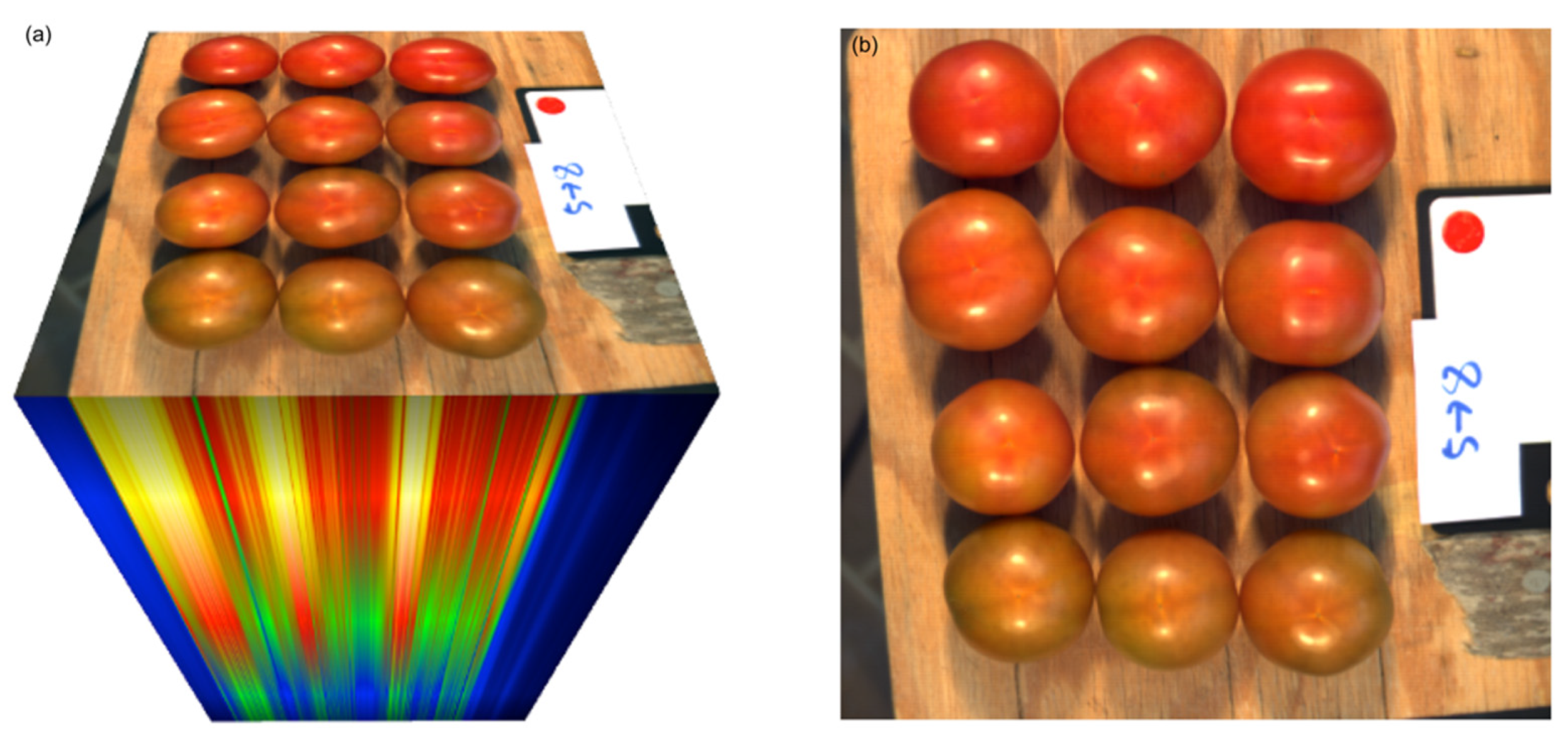
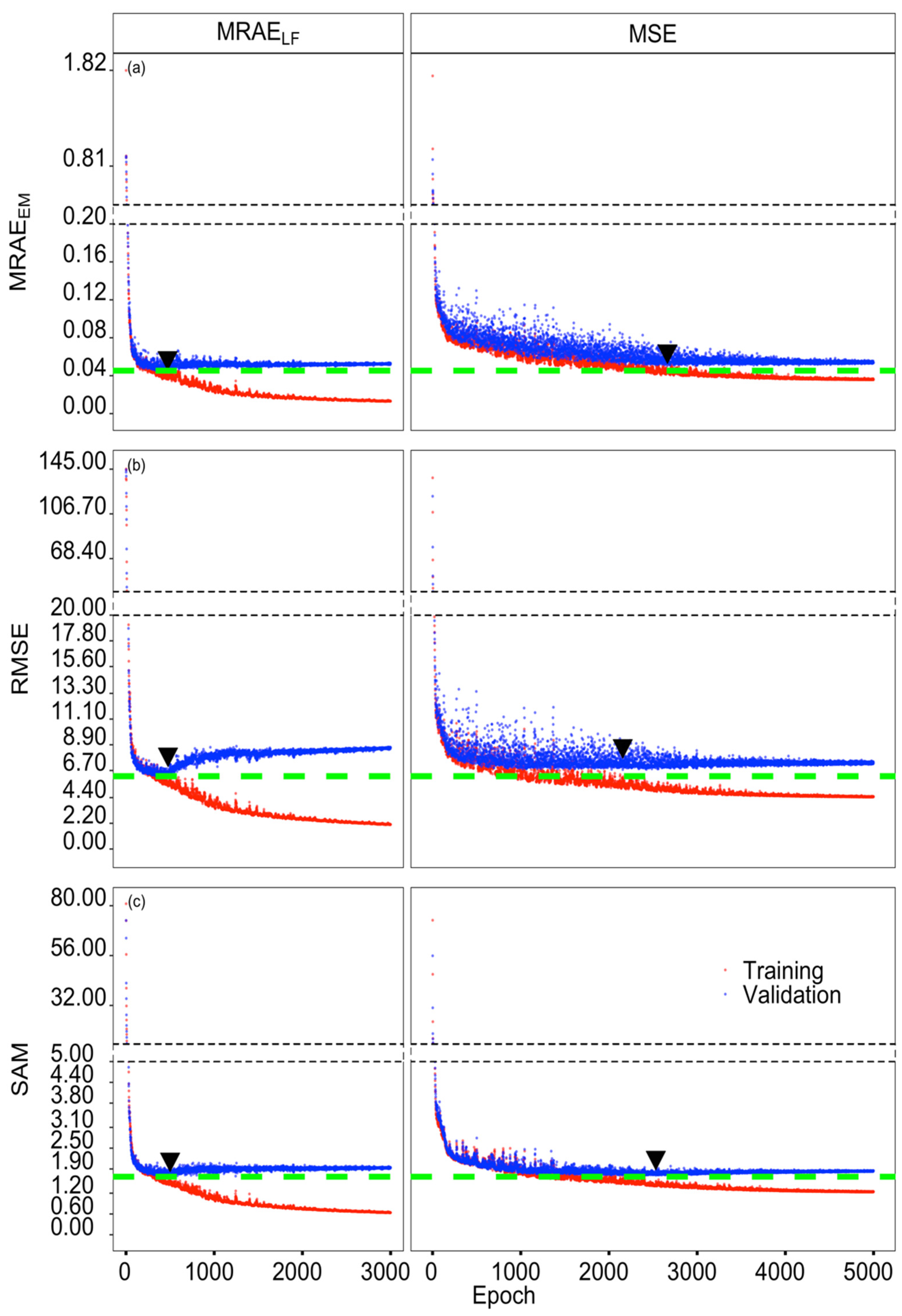
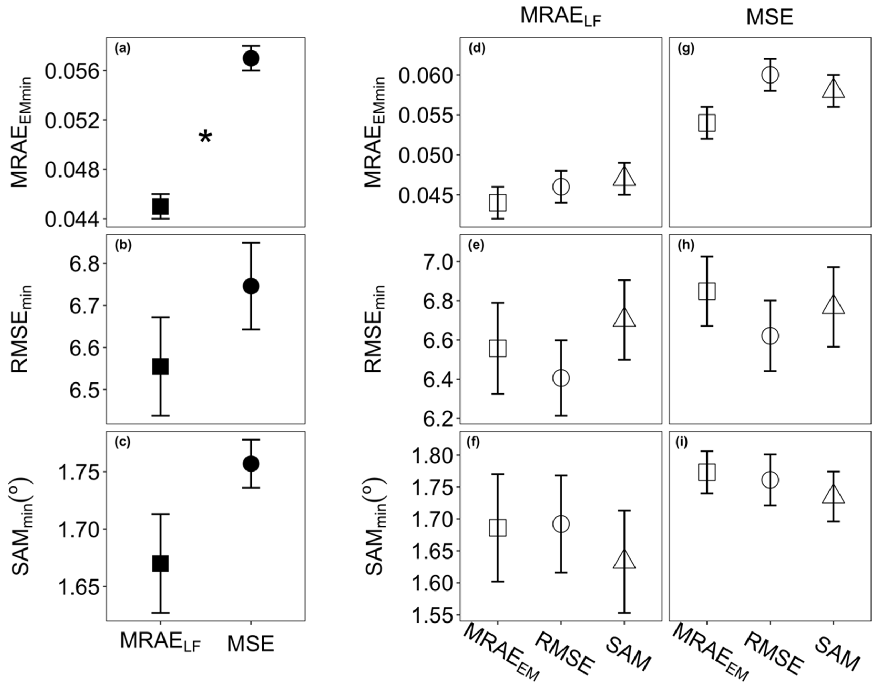
3.1. Model Selection and Performance
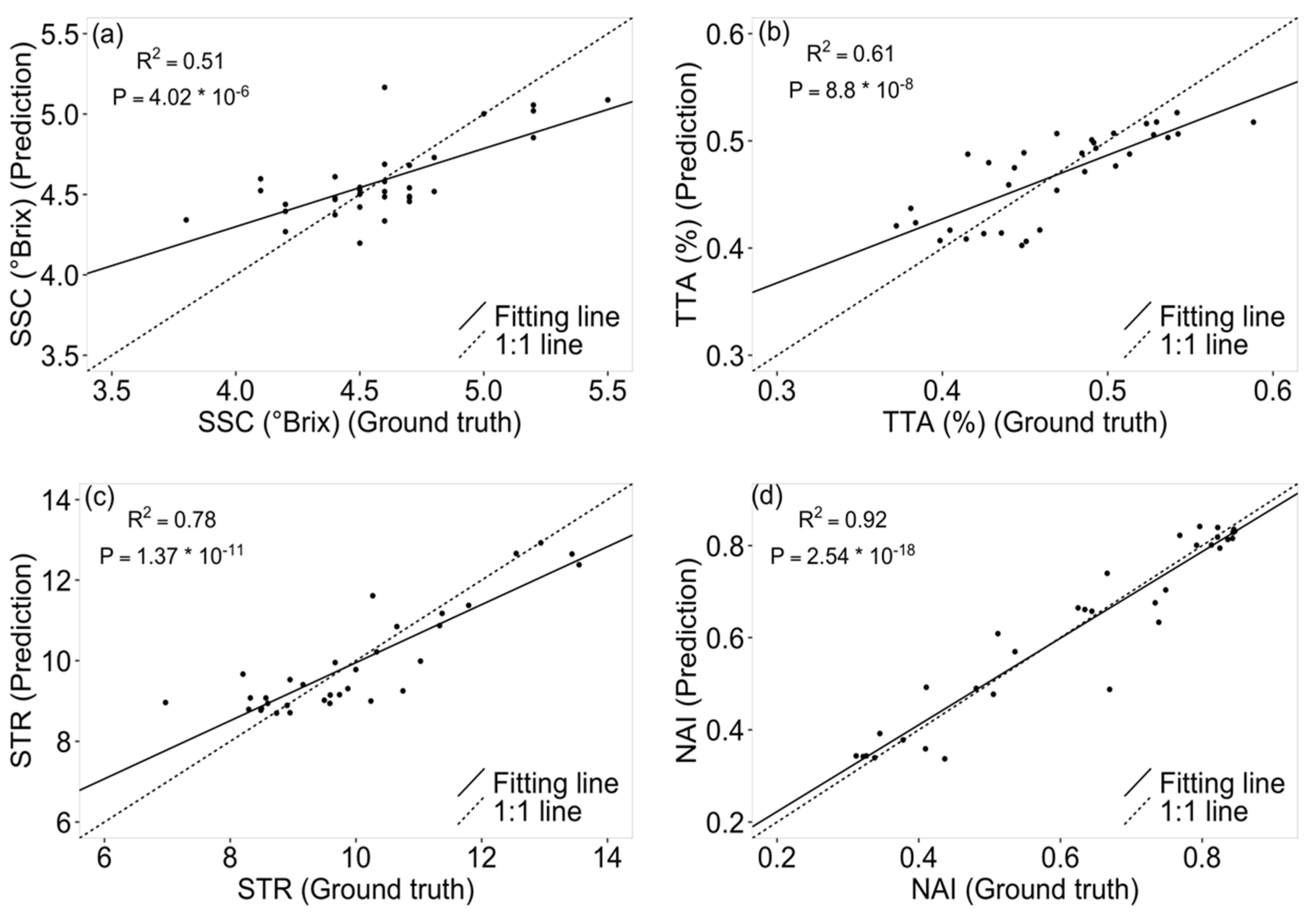
3.2. Tomato Quality Parameter Prediction
4. Discussion
5. Conclusions
Supplementary Materials
Author Contributions
Funding
Acknowledgments
Conflicts of Interest
References
- Dong, X.; Jakobi, M.; Wang, S.; Köhler, M.H.; Zhang, X.; Koch, A.W. A review of hyperspectral imaging for nanoscale materials research. Appl. Spectrosc. Rev. 2019, 54, 285–305. [Google Scholar] [CrossRef]
- Cozzolino, D.; Murray, I. Identification of animal meat muscles by visible and near infrared reflectance spectroscopy. LWT Food Sci. Technol. 2004, 37, 447–452. [Google Scholar] [CrossRef]
- Mahlein, A.K.; Kuska, M.T.; Thomas, S.; Bohnenkamp, D.; Alisaac, E.; Behmann, J.; Wahabzada, M.; Kersting, K. Plant disease detection by hyperspectral imaging: From the lab to the field. Adv. Anim. Biosci. 2017, 8, 238–243. [Google Scholar] [CrossRef]
- Qi, H.; Paz-Kagan, T.; Karnieli, A.; Jin, X.; Li, S. Evaluating calibration methods for predicting soil available nutrients using hyperspectral VNIR data. Soil Tillage Res. 2018, 175, 267–275. [Google Scholar] [CrossRef]
- Vance, C.K.; Tolleson, D.R.; Kinoshita, K.; Rodriguez, J.; Foley, W.J. Near infrared spectroscopy in wildlife and biodiversity. J. Near Infrared Spectrosc. 2016, 24, 1–25. [Google Scholar] [CrossRef]
- Afara, I.O.; Prasadam, I.; Arabshahi, Z.; Xiao, Y.; Oloyede, A. Monitoring osteoarthritis progression using near infrared (NIR) spectroscopy. Sci. Rep. 2017, 7, 11463. [Google Scholar] [CrossRef] [PubMed]
- Tsuchikawa, S.; Kobori, H. A review of recent application of near infrared spectroscopy to wood science and technology. J. Wood Sci. 2015, 61, 213–220. [Google Scholar] [CrossRef]
- Barbin, D.F.; ElMasry, G.; Sun, D.-W.; Allen, P.; Morsy, N. Non-destructive assessment of microbial contamination in porcine meat using NIR hyperspectral imaging. Innov. Food Sci. Emerg. Technol. 2013, 17, 180–191. [Google Scholar] [CrossRef]
- Menesatti, P.; Antonucci, F.; Pallottino, F.; Giorgi, S.; Matere, A.; Nocente, F.; Pasquini, M.; D’Egidio, M.G.; Costa, C. Laboratory vs. in-field spectral proximal sensing for early detection of Fusarium head blight infection in durum wheat. Biosyst. Eng. 2013, 114, 289–293. [Google Scholar] [CrossRef]
- Signoroni, A.; Savardi, M.; Baronio, A.; Benini, S. Deep learning meets hyperspectral image analysis: A multidisciplinary review. J. Imaging 2019, 5, 52. [Google Scholar] [CrossRef]
- Cao, X.; Du, H.; Tong, X.; Dai, Q.; Lin, S. A prism-mask system for multispectral video acquisition. IEEE Trans. Pattern Anal. Mach. Intell. 2011, 33, 2423–2435. [Google Scholar]
- Thomas, S.; Kuska, M.T.; Bohnenkamp, D.; Brugger, A.; Alisaac, E.; Wahabzada, M.; Behmann, J.; Mahlein, A.-K. Benefits of hyperspectral imaging for plant disease detection and plant protection: A technical perspective. J. Plant Dis. Prot. 2018, 125, 5–20. [Google Scholar] [CrossRef]
- Rahimy, E. Deep learning applications in ophthalmology. Curr. Opin. Ophthalmol. 2018, 29, 254–260. [Google Scholar] [CrossRef] [PubMed]
- Rao, Q.; Frtunikj, J. Deep learning for self-driving cars: Chances and challenges. In Proceedings of the 1st International Workshop on Software Engineering for AI in Autonomous Systems, Gothenburg, Sweden, 28 May 2018; pp. 35–38. [Google Scholar]
- Ghosal, S.; Zheng, B.; Chapman, S.C.; Potgieter, A.B.; Jordan, D.R.; Wang, X.; Singh, A.K.; Singh, A.; Hirafuji, M.; Ninomiya, S. A weakly supervised deep learning framework for sorghum head detection and counting. Plant Phenomics 2019, 2019, 1525874. [Google Scholar] [CrossRef]
- Xiong, Z.; Shi, Z.; Li, H.; Wang, L.; Liu, D.; Wu, F. HSCNN: CNN-based hyperspectral image recovery from spectrally undersampled projections. In Proceedings of the IEEE International Conference on Computer Vision, Venice, Italy, 22–29 October 2017; pp. 518–525. [Google Scholar]
- Shi, Z.; Chen, C.; Xiong, Z.; Liu, D.; Wu, F. HSCNN+: Advanced CNN-based hyperspectral recovery from rgb images. In Proceedings of the IEEE Conference on Computer Vision and Pattern Recognition Workshops, Salt Lake City, UT, USA, 18–22 June 2018; pp. 939–947. [Google Scholar]
- Arad, B.; Ben-Shahar, O. Sparse recovery of hyperspectral signal from natural RGB images. In Proceedings of the European Conference on Computer Vision; Springer: New York, NY, USA, 2016; pp. 19–34. [Google Scholar]
- Galliani, S.; Lanaras, C.; Marmanis, D.; Baltsavias, E.; Schindler, K. Learned spectral super-resolution. arXiv 2017, arXiv:1703.09470. [Google Scholar]
- Tschannerl, J.; Ren, J.; Marshall, S. Low cost hyperspectral imaging using deep learning based spectral reconstruction. Lect. Notes Comput. Sci. (Including Subser. Lect. Notes Artif. Intell. Lect. Notes Bioinformatics) 2018, 11257 LNCS, s 206–s 217. [Google Scholar]
- Stiebel, T.; Koppers, S.; Seltsam, P.; Merhof, D. Reconstructing spectral images from rgb-images using a convolutional neural network. In Proceedings of the IEEE/CVF Conference on Computer Vision and Pattern Recognition Workshops (CVPRW), Salt Lake City, UT, USA, 18–22 June 2018; pp. 948–953. [Google Scholar]
- Nie, S.; Gu, L.; Zheng, Y.; Lam, A.; Ono, N.; Sato, I. Deeply learned filter response functions for hyperspectral reconstruction. In Proceedings of the IEEE Conference on Computer Vision and Pattern Recognition, Salt Lake City, UT, USA, 18–22 June 2018; pp. 4767–4776. [Google Scholar]
- Nagasubramanian, K.; Jones, S.; Singh, A.K.; Sarkar, S.; Singh, A.; Ganapathysubramanian, B. Plant disease identification using explainable 3D deep learning on hyperspectral images. Plant Methods 2019, 15, 98. [Google Scholar] [CrossRef] [PubMed]
- Can, Y.B.; Timofte, R. An efficient CNN for spectral reconstruction from RGB images. arXiv 2018, arXiv:1804.04647. [Google Scholar]
- Yan, Y.; Zhang, L.; Li, J.; Wei, W.; Zhang, Y. Accurate Spectral Super-Resolution from Single RGB Image Using Multi-scale CNN. In Pattern Recognition and Computer Vision; Lai, J.H., Liu, C.L., Chen, X., Zhou, J., Tan, T., Zheng, N., Zha, H., Eds.; Springer International Publishing: Cham, Switzerland, 2018; pp. 206–217. [Google Scholar]
- Ma, J.; Sun, D.-W.; Pu, H.; Cheng, J.-H.; Wei, Q. Advanced techniques for hyperspectral imaging in the food industry: Principles and recent applications. Annu. Rev. Food Sci. Technol. 2019, 10, 197–220. [Google Scholar] [CrossRef] [PubMed]
- Jiang, F.; Lopez, A.; Jeon, S.; de Freitas, S.T.; Yu, Q.; Wu, Z.; Labavitch, J.M.; Tian, S.; Powell, A.L.T.; Mitcham, E. Disassembly of the fruit cell wall by the ripening-associated polygalacturonase and expansin influences tomato cracking. Hortic. Res. 2019, 6, 17. [Google Scholar] [CrossRef]
- Polder, G.; Van Der Heijden, G.; Van der Voet, H.; Young, I.T. Measuring surface distribution of carotenes and chlorophyll in ripening tomatoes using imaging spectrometry. Postharvest Biol. Technol. 2004, 34, 117–129. [Google Scholar] [CrossRef]
- Simonne, A.H.; Fuzere, J.M.; Simonne, E.; Hochmuth, R.C.; Marshall, M.R. Effects of nitrogen rates on chemical composition of yellow grape tomato grown in a subtropical climate. J. Plant Nutr. 2007, 30, 927–935. [Google Scholar] [CrossRef]
- Qin, J.; Chao, K.; Kim, M.S. Investigation of Raman chemical imaging for detection of lycopene changes in tomatoes during postharvest ripening. J. Food Eng. 2011, 107, 277–288. [Google Scholar] [CrossRef]
- Clément, A.; Dorais, M.; Vernon, M. Nondestructive measurement of fresh tomato lycopene content and other physicochemical characteristics using visible—NIR spectroscopy. J. Agric. Food Chem. 2008, 56, 9813–9818. [Google Scholar] [CrossRef]
- Akinaga, T.; Tanaka, M.; Kawasaki, S. On-tree and after-harvesting evaluation of firmness, color and lycopene content of tomato fruit using portable NIR spectroscopy. J. Food Agric. Environ. 2008, 6, 327–332. [Google Scholar]
- Huang, Y.; Lu, R.; Chen, K. Assessment of tomato soluble solids content and pH by spatially-resolved and conventional Vis/NIR spectroscopy. J. Food Eng. 2018, 236, 19–28. [Google Scholar] [CrossRef]
- Ntagkas, N.; Min, Q.; Woltering, E.J.; Labrie, C.; Nicole, C.C.S.; Marcelis, L.F.M. Illuminating tomato fruit enhances fruit vitamin C content. In Proceedings of the VIII International Symposium on Light in Horticulture 1134, East Lansing, MI, USA, 22–26 May 2016; pp. 351–356. [Google Scholar]
- Farneti, B.; Schouten, R.E.; Woltering, E.J. Low temperature-induced lycopene degradation in red ripe tomato evaluated by remittance spectroscopy. Postharvest Biol. Technol. 2012, 73, 22–27. [Google Scholar] [CrossRef]
- Farinetti, A.; Zurlo, V.; Manenti, A.; Coppi, F.; Mattioli, A.V. Mediterranean diet and colorectal cancer: A systematic review. Nutrition 2017, 43, 83–88. [Google Scholar] [CrossRef]
- Chandrasekaran, I.; Panigrahi, S.S.; Ravikanth, L.; Singh, C.B. Potential of Near-Infrared (NIR) spectroscopy and hyperspectral imaging for quality and safety assessment of fruits: An overview. Food Anal. Methods 2019, 12, 2438–2458. [Google Scholar] [CrossRef]
- Paponov, M.; Kechasov, D.; Lacek, J.; Verheul, M.; Paponov, I.A. Supplemental LED inter-lighting increases tomato fruit growth through enhanced photosynthetic light use efficiency and modulated root activity. Front. Plant Sci. 2020, 10, 1656. [Google Scholar] [CrossRef]
- Cantwell, M. Optimum procedures for ripening tomatoes. Manag. Fruit Ripening Postharvest Hortic. Ser. 2000, 9, 80–88. [Google Scholar]
- Behmann, J.; Acebron, K.; Emin, D.; Bennertz, S.; Matsubara, S.; Thomas, S.; Bohnenkamp, D.; Kuska, M.; Jussila, J.; Salo, H. Specim IQ: Evaluation of a new, miniaturized handheld hyperspectral camera and its application for plant phenotyping and disease detection. Sensors 2018, 18, 441. [Google Scholar] [CrossRef]
- Mitcham, B.; Cantwell, M.; Kader, A. Methods for determining quality of fresh commodities. Perishables Handl. Newsl. 1996, 85, 1–5. [Google Scholar]
- Verheul, M.J.; Slimestad, R.; Tjøstheim, I.H. From producer to consumer: Greenhouse tomato quality as affected by variety, maturity stage at harvest, transport conditions, and supermarket storage. J. Agric. Food Chem. 2015, 63, 5026–5034. [Google Scholar] [CrossRef] [PubMed]
- Yamamoto, K.; Guo, W.; Yoshioka, Y.; Ninomiya, S. On plant detection of intact tomato fruits using image analysis and machine learning methods. Sensors 2014, 14, 12191–12206. [Google Scholar] [CrossRef] [PubMed]
- He, K.; Zhang, X.; Ren, S.; Sun, J. Deep residual learning for image recognition. In Proceedings of the IEEE conference on computer vision and pattern recognition, Las Vegas, NV, USA, 26 June–1 July 2016; pp. 770–778. [Google Scholar]
- Renza, D.; Martinez, E.; Molina, I. Unsupervised change detection in a particular vegetation land cover type using spectral angle mapper. Adv. Sp. Res. 2017, 59, 2019–2031. [Google Scholar] [CrossRef]
- Kingma, D.P.; Ba, J. Adam: A method for stochastic optimization. arXiv 2014, arXiv:1412.6980. [Google Scholar]
- Millard, S.P.; Kowarik, M.A.; Imports, M. Package ‘EnvStats’. Packag. Environ. Stat. Version 2018, 2, 31–32. [Google Scholar]
- R Core Team. R: A Language and Environment for Statistical Computing; R Foundation for Statistical Computing: Vienna, Austria, 2013. [Google Scholar]
- Russell, B.C.; Torralba, A.; Murphy, K.P.; Freeman, W.T. LabelMe: A database and web-based tool for image annotation. Int. J. Comput. Vis. 2008, 77, 157–173. [Google Scholar] [CrossRef]
- Lin, T.-Y.; Goyal, P.; Girshick, R.; He, K.; Dollár, P. Focal loss for dense object detection. In Proceedings of the IEEE International Conference on Computer Vision (ICCV), Venice, Italy, 22–29 October 2017; pp. 2999–3007. [Google Scholar]
- Esquerre, C.; Gowen, A.A.; Burger, J.; Downey, G.; O’Donnell, C.P. Suppressing sample morphology effects in near infrared spectral imaging using chemometric data pre-treatments. Chemom. Intell. Lab. Syst. 2012, 117, 129–137. [Google Scholar] [CrossRef]
- Liu, W.; Lee, J. An Efficient Residual Learning Neural Network for Hyperspectral Image Superresolution. IEEE J. Sel. Top. Appl. Earth Obs. Remote Sens. 2019, 12, 1240–1253. [Google Scholar] [CrossRef]
- Martin-Diaz, I.; Morinigo-Sotelo, D.; Duque-Perez, O.; de J. Romero-Troncoso, R. Early fault detection in induction motors using AdaBoost with imbalanced small data and optimized sampling. IEEE Trans. Ind. Appl. 2016, 53, 3066–3075. [Google Scholar] [CrossRef]
- Kozukue, N.; Friedman, M. Tomatine, chlorophyll, β-carotene and lycopene content in tomatoes during growth and maturation. J. Sci. Food Agric. 2003, 83, 195–200. [Google Scholar] [CrossRef]
- Schouten, R.E.; Farneti, B.; Tijskens, L.M.M.; Alarcón, A.A.; Woltering, E.J. Quantifying lycopene synthesis and chlorophyll breakdown in tomato fruit using remittance VIS spectroscopy. Postharvest Biol. Technol. 2014, 96, 53–63. [Google Scholar] [CrossRef]
- Singh, L.; Mutanga, O.; Mafongoya, P.; Peerbhay, K. Remote sensing of key grassland nutrients using hyperspectral techniques in KwaZulu-Natal, South Africa. J. Appl. Remote Sens. 2017, 11, 36005. [Google Scholar] [CrossRef]
- Kawamura, K.; Tsujimoto, Y.; Rabenarivo, M.; Asai, H.; Andriamananjara, A.; Rakotoson, T. Vis-NIR spectroscopy and PLS regression with waveband selection for estimating the total C and N of paddy soils in Madagascar. Remote Sens. 2017, 9, 1081. [Google Scholar] [CrossRef]


| Loss Function | Epoch | Time (s) | MRAEEM | RMSE | SAM (°) |
|---|---|---|---|---|---|
| MRAELF | 472 | 83.57 | 0.0453 | 6.264 | 1.743 |
| 476 | 84.29 | 0.0454 | 6.223 | 1.723 | |
| 500 | 88.58 | 0.0513 | 7.053 | 1.676 | |
| MSE | 2663 | 497.49 | 0.0507 | 7.157 | 1.773 |
| 2156 | 404.69 | 0.0554 | 6.778 | 1.761 | |
| 2531 | 473.56 | 0.0570 | 6.922 | 1.735 |
© 2020 by the authors. Licensee MDPI, Basel, Switzerland. This article is an open access article distributed under the terms and conditions of the Creative Commons Attribution (CC BY) license (http://creativecommons.org/licenses/by/4.0/).
Share and Cite
Zhao, J.; Kechasov, D.; Rewald, B.; Bodner, G.; Verheul, M.; Clarke, N.; Clarke, J.L. Deep Learning in Hyperspectral Image Reconstruction from Single RGB images—A Case Study on Tomato Quality Parameters. Remote Sens. 2020, 12, 3258. https://doi.org/10.3390/rs12193258
Zhao J, Kechasov D, Rewald B, Bodner G, Verheul M, Clarke N, Clarke JL. Deep Learning in Hyperspectral Image Reconstruction from Single RGB images—A Case Study on Tomato Quality Parameters. Remote Sensing. 2020; 12(19):3258. https://doi.org/10.3390/rs12193258
Chicago/Turabian StyleZhao, Jiangsan, Dmitry Kechasov, Boris Rewald, Gernot Bodner, Michel Verheul, Nicholas Clarke, and Jihong Liu Clarke. 2020. "Deep Learning in Hyperspectral Image Reconstruction from Single RGB images—A Case Study on Tomato Quality Parameters" Remote Sensing 12, no. 19: 3258. https://doi.org/10.3390/rs12193258
APA StyleZhao, J., Kechasov, D., Rewald, B., Bodner, G., Verheul, M., Clarke, N., & Clarke, J. L. (2020). Deep Learning in Hyperspectral Image Reconstruction from Single RGB images—A Case Study on Tomato Quality Parameters. Remote Sensing, 12(19), 3258. https://doi.org/10.3390/rs12193258