Tailored Algorithms for the Detection of the Atmospheric Boundary Layer Height from Common Automatic Lidars and Ceilometers (ALC)

Abstract

A detailed understanding of atmospheric boundary layer (ABL) processes is key to improve forecasting of pollution dispersion and cloud dynamics in the context of future climate scenarios. International networks of automatic lidars and ceilometers (ALC) are gathering valuable data that allow for the height of the ABL and its sublayers to be derived in near real time. A new generation of advanced methods to automatically detect the ABL heights now exist. However, diversity in ALC models means these algorithms need to be tailored to instrument-specific capabilities. Here, the advanced algorithm STRATfinder is presented for application to high signal-to-noise ratio (SNR) ALC observations, and results are compared to an automatic algorithm designed for low-SNR measurements (CABAM). The two algorithms are evaluated for application in an operational network setting. Results indicate that the ABL heights derived from low-SNR ALC have increased uncertainty during daytime deep convection, while high-SNR observations can have slightly reduced capabilities in detecting shallow nocturnal layers. Agreement between the ALC-based methods is similar when either is compared to the ABL heights derived from temperature profile data. The two independent methods describe very similar average diurnal and seasonal variations. Hence, high-quality products of ABL heights may soon become possible at national and continental scales.

1. Introduction

Automatic lidars and ceilometers (ALC) are operated in dense networks to monitor cloud base height (CBH) for the support of surface-based weather observations (e.g., at airports) and the evaluation of numerical weather prediction models [1]. With recent advances in measurement technology and algorithm development [2], high quality attenuated backscatter profiles are increasingly recorded by ALC networks. These observations allow for the detection of aerosol layers [3] and the height of the atmospheric boundary layer (ABL) and its sublayers to be determined [4,5]. More long-term observations of the ABL heights in a variety of geographical settings are urgently needed, e.g., for the interpretation of near-surface pollutant concentrations [6,7,8], model evaluation [9], and carbon budget assessment [10,11].

To automatically derive ABL heights from ALC observations, advanced methods have been developed, with ‘second-generation’ algorithms (e.g., [12,13,14,15,16,17,18,19,20,21,22]) now becoming available. The two steps of analysis involve: (1) examination of recorded attenuated backscatter profiles for regions of significant change indicating layer boundaries and (2) layer attribution to determine the type of ABL sublayer. The task of layer attribution has been identified as the main challenge for the automatic detection of ABL heights [16]. The most pronounced layer boundary usually occurs between the ABL and the free troposphere above, defining the height of the ABL (ABLH). Sublayers such as the mixed layer and the residual layer (RL) can be distinguished. Here, the term “mixed layer” is used to describe the lowest atmospheric layer in which aerosols and moisture are dispersed by recent mixing processes during both night and day. The layer may be of any atmospheric stability. The mixed layer height (MLH) marks the boundary to the residual layer and, when the mixed layer extends over the whole ABL, MLH equals ABLH.

It has been demonstrated that uncertainties in the observed attenuated backscatter differ between ALC models [23] but also may depend on the specific hardware and software setup [24]. Data processing and correction procedures have been developed recently (e.g., [24,25]) that allow for the harmonization of attenuated backscatter observations from various sensors. Still, instrument specifics mean ALC commonly deployed in national and international measurement networks do not always have the same capabilities. Two critical sensor-related issues for detection of the ABL heights are the following:

(a)

The signal-to-noise ratio (SNR) determines how well layers can be detected. SNR depends on the composition of the probed atmosphere (amount of aerosol, moisture) and the lidar system [26]. Relatively high noise can create false signatures in the attenuated backscatter that may be mistaken for a physical layer boundary. As the signal returned to the detector from a homogeneous atmosphere decreases with increasing distance from the sensor (i.e., range), ALC with inherently lower power and/or higher noise associated with the lidar system provide particularly low SNR observations not only for reduced aerosol load but also during deep ABL convection. This increases the uncertainties in detection of ABL heights.

(b)

Some ALC have a large ‘blind zone’ or greater uncertainty in the very near range due to the incomplete optical overlap between the transmitter and receiver unit. This limits the detection of shallow layers within the ABL, which often occur with stable atmospheric stratification at night. Other ALC have a near-complete optical overlap, allowing shallow layers (< 100 m above ground level, agl) to be derived.

Commonly deployed ALC can be split into low- and high-SNR sensors, with varying optical overlap and near-range uncertainties. To obtain spatially consistent data products, the EUMETNET E-PROFILE program [27] is developing tools for application to ground-based profiling networks (https://e-profile.eu). To best exploit the respective capabilities of high-SNR and low-SNR ALC types, tailored algorithms (Section 2) are proposed for application in a network setting such as E-PROFILE. STRATfinder, a high-SNR ALC algorithm, combines advantages from both STRAT-2D/STRAT+ [14,15,16] and pathfinderTURB [22]. The CABAM algorithm [17,28] for low-SNR ALC has been made more flexible for network application. The algorithms are applied to long-term datasets gathered by high-SNR and low-SNR ALC sensors co-located at two sites with differing ABL characteristics. Results are evaluated against thermodynamic ABL indicators, before their agreement is assessed for individual measurement periods and based on their ability to capture diurnal and seasonal average ABL heights (Section 3). Applicability of the algorithms to other ALC models is discussed and site and sensor specific considerations for the implementation of automatic MLH detection across a diverse network are identified (Section 4) before overall conclusions are summarised (Section 5).

2. Materials and Methods

Two tailored algorithms are evaluated for application in a network setting: STRATfinder for high-SNR (Section 2.1) and CABAM for low-SNR ALC data processing (Section 2.2). Both rely solely on ALC observations, i.e., profiles of attenuated backscatter and CBH. Additional quality control steps are implemented to flag physically unreasonable MLH results obtained by either of the two methods (Section 2.3). For independent reference, thermodynamic ABL heights are determined from Aircraft Meteorological Data Relay (AMDAR) profile observations (Section 2.4). The evaluation is performed based on observations at two E-PROFILE stations (Section 2.5).

2.1. STRATfinder for High-SNR ALC

STRATfinder tracks MLH and ABLH, providing a full picture of the boundary layer configuration over a 24 h period at 1 min resolution. Layers are traced using the graph-based “pathfinder” [13] approach, which determines the optimised “path” between two points in a two-dimensional field of “weights” by minimising a cost function. More details on the ‘pathfinder’ method are provided in previous studies [13,22]. High weights are defined within the mixed layer and residual layer, while regions with low weights guide the path along the layer boundaries. Weights are low where strong negative vertical gradients in attenuated backscatter occur. The high SNR allows for the temporal variance introduced by entrainment at the top of the mixed layer [15] to be exploited. As variance is particularly strong at the top of the mixed layer during the morning growth and during daytime when air from the residual layer or the free troposphere is being mixed into the lowest atmospheric layer, a second field of weights is defined by the inverse of the attenuated backscatter variance so that low weights again mark the top of the mixed layer. The search regions for ABLH and MLH are restricted by pre-defined limits (Appendix A).

STRATfinder (written in MATLAB version 2017b, licensed under the GNU General Public License v3.0) uses the following steps (Figure 1):

• The temporal variance field is calculated from 15 s data at block intervals and window length defined by the user (

  Table A1. STRATfinder algorithm input parameters used. As the signal recorded by the ALC is not absolutely calibrated into units of attenuated backscatter [46,47], signal-related thresholds are here specified in arbitrary units (a.u.). See Poltera et al. [22] for details on variance calculations.

  Group	Parameter Name	Description	Value Used in This Study
  Calculation	min	Minimum height considered	0 m agl
  	max	Maximum height considered	4500 m agl
  Cloud	window	Window size to smooth attenuated backscatter when creating cloud mask before variance calculations	11 time steps
  	threshold	Attenuated backscatter exceeding this value is excluded from variance calculations	107 a.u.
  Instrument	threshold_overlap	Profile only considered above this limit of optical overlap function	5%
  MLHsettings	threshold_molecular	Threshold used to identify lowest height in attenuated backscatter profile where signal particle scattering is negligible. Used to define upper search region for ABLH.	104.6 a.u.
  	dayMax	Maximum of ABLH search region during day	4000 m agl
  	dayMin	Minimum of ABLH search region during day	0 m agl
  	evening	Maximum of ABLH search region during evening	2500 m agl
  	nightMax	Maximum of MLH search region during night	700 m agl
  	nightMin	Maximum of MLH search region during night	0 m agl
  	growth_onset	Delay of growth onset relative to sunrise	10800 s
  	growth_rate	Growth rate considered up from onset to define maximum search region of MLH	300 m h−1
  	jump	Maximum allowed vertical displacement between two adjacent paths tracked by pathfinding algorithm	32.5 m
  	threshold_gradient	Threshold to define regions of increased weights based on small or positive vertical gradients	−5 ∙ 10−4 a.u.
  	threshold_log10variance	Threshold to define regions of increased weights based on low variance	1010
  Pathfinder	window	Period considered for each implementation of pathfinding algorithm	1800 s
  Variance	highpassfilter	Wavelength above with variance contributions are omitted	1800 s
  	FFT_window	Time window for variance calculations	3600 s
  	FFT_sample	Time resolution for variance calculations	600 s

  ). Here, variance is calculated every 10 min over sliding windows of 1 h to capture the essential spectral information content. To avoid high signals associated with clouds introducing additional variability, a moving average with range (height) is calculated. Any instance exceeding a set threshold (Table A1) is excluded from the calculations. Subsequently, attenuated backscatter observations are detrended and a high-pass filter applied with a cut off to remove meso-scale variations [22]. Finally, variance is estimated using a fast Fourier transform function [22].
• To standardise the output, attenuated backscatter is block-averaged to a temporal resolution of 1 min and a range resolution of 30 m. Range is converted to height above ground level (agl) accounting for the beam tilt angle. A smooth field of attenuated backscatter is generated using gaussian blur and 2D anisotropic diffusion [22].
• Vertical gradients are calculated from the log₁₀ of the smoothed attenuated backscatter.
• Two weights fields are estimated: (1) inverse of the vertical gradient field and (2) combined gradient and variance indicators. High weights are set to block the path where vertical gradients are positive or small in magnitude and variance is low.
• Several characteristic heights are specified by the user to define the limits constraining the search regions for ABLH and MLH. An auxiliary layer height (XLH) is tracked backwards in time from midnight to noon to assist MLH detection during the evening decay of the mixed layer.
• The Dijkstra algorithm [29] is applied to track MLH, XLH, and ABLH. The path minimises the cost function across a user-defined time window (Table A1). Individual paths are connected to determine MLH and ABLH for the whole 24 h period. ABLH detection relies on the weights specified by the gradient field, as does the tracking of XLH and MLH detection before the morning growth onset. To detect the MLH between the morning growth and midnight, the weights field combining gradient and variance characteristics is used. At the start of each layer search, the first vertical profile of weights is evaluated for local minima (with N_min = number of local minima). If an ABLH estimate is already available from the previous day, the starting point for the ABLH search is set to the last height of this layer, or otherwise to the (N_min∙0.75)^th local minimum. Search for MLH and XLH starts at the height of the (N_min∙0.25)^th local minimum. For every consecutive search window, the end point of the layer detected in the prior window is used as the starting point. At times, no reasonable path is traceable to significant negative vertical gradients in attenuated backscatter. When this occurs, the whole search window is removed from final output by applying an overall threshold to the cost of a given path.
• The auxiliary layer XLH and the preliminary MLH are merged to give the final MLH estimate. If the difference between the first and maximum XLH is smaller than the minimum difference between XLH and MLH, MLH is set to XLH up from sunset. Otherwise, the two layers are connected from the point where they are in shortest distance to each other. Intermediate results of XLH (MLH) before (after) that connection point are discarded.
• If the variance exceeds a threshold (Table A1) for 75% of the profile below CBH, precipitation is considered to impede successful layer detection and tracking of both MLH and ABLH is interrupted.

While STRAT-2D/STRAT+ and pathfinderTURB have been evaluated against ABLH estimates from radiosondes and expert manual detection [15,22], the new STRATfinder (version 2019.3) has not yet been assessed. Compared to STRAT-2D/STRAT+, STRATfinder’s main advantages are the implementation of the pathfinding algorithm and the definition of reasonable boundaries for the search region. The main advantage of STRATfinder compared to pathfinderTURB is its simplicity, more user-friendly setup, and its applicability to a 24 h period (pathfinderTURB only has daytime MLH detection capability).

2.2. CABAM for Low-SNR ALC

The CABAM algorithm, developed for low-SNR ALC observations [17], tracks MLH and additional layers forming the RL, while taking into account the presence of clouds. Following the detection of significant vertical gradients in the attenuated backscatter profiles, layers are connected using a dynamic decision-tree with rules varying through the day. As precipitation hinders MLH detection, affected periods are filtered out automatically, using indicators derived from attenuated backscatter profiles. A first-order estimate of ABLH is calculated as the median of all layers recorded at any given timestep. Automatic layer detection and attribution are performed at the raw resolution of the data, and final results are block-averaged to 15 min (time ending). The code is written in R [30]. In addition to the MLH and RL detection, CABAM includes a module to classify ABL conditions by cloud cover and cloud type (convective or stratiform) [28]. MLH results were successfully evaluated against independent reference measurements [17] and compared to mixing heights derived from Doppler lidar profiles [31].

CABAM algorithm improvements (version 2019.3) include: a more dynamic near-range module [17], more flexibility for network use, and a new module (Supplementary Materials S.1) to improve performance during deep convection (>2000 m) when the ALC’s low SNR frequently leads to false layer detection within the ABL and thereby a systematic under-estimation of daytime MLH.

2.3. Quality Control

As both methods, STRATfinder (Section 2.1) and CABAM (Section 2.2), occasionally yield physically unreasonable MLH results, additional post-processing quality control steps are implemented:

• Low MLH caused by precipitation: Although both methods aim to assess if precipitation is hindering MLH detection, results still include periods during or after rainfall affecting the ALC measurements leading to low MLH. For STRATfinder, MLH below the 15^th percentile statistics by season (winter = DJF, spring = MAM, summer = JJA, and autumn = SON) and time relative to sunrise based on all available results (Section 3.1) are flagged if precipitation is detected within a 45 min window of the interval or if more than 2 h of a day are flagged to be severely affected by precipitation. Gaps of up to 2 h between these flagged periods are also flagged. For CABAM, days (sunrise until sunset) or nights (sunset until sunrise) with more than 3 h of precipitation inhibiting successful MLH detection are flagged completely.
• At times, the CABAM near-range module does not successfully discard some candidate layers below 200 m. STRATfinder search limits falsely allow a path near the overlap-related minimum detection limit to be followed. These false layer detections by either algorithm result in layers with hardly any variability in layer height below 300 m even during daytime when turbulent exchange clearly establishes a convective boundary layer above (as is evident from manual inspection of the attenuated backscatter). Such daytime conditions are flagged between March and October if more than 50% of the MLH results h later than 5 h after sunrise remain below 300 m or if MLH actually exceeds 450 m at some time between sunrise and solar noon, and MLH then falls again below 300 m before sunset.
• Both methods occasionally show MLH temporal inconsistencies (i.e., very unlikely changes in magnitude). If the MLH increase (decrease) at midnight is greater than 500 m, periods between midnight and sunrise (sunset and midnight) are flagged. Further, if MLH increases by more than 500 m 15 min⁻¹ at any other time during the night, periods are flagged either up to a decrease by more than 500 m 15 min⁻¹ or up to sunrise if no strong decrease occurs. If the MLH increases by more than 500 m 15 min⁻¹ before 4 h after sunrise, the periods until 4 h after sunrise are flagged.
• The relation between CBH and MLH is used to assess potential false layer attribution by CABAM. If CBH indicates clouds are forming at the top of the ABL before 2 h prior to sunset and MLH is found more than 200 m below the CBH for a time window of at least 1 h, MLH is flagged as a likely underestimation.
• If no clear nocturnal boundary layer near the ground is detected, CABAM results during the night may represent the residual layer during spring and summer. If the minimum MLH in the three hours before sunrise is located above 900 m, MLH up to 3 h after sunrise is flagged. Or if MLH exceeds 2000 m within 5 h of sunrise, MLH greater than this height is flagged for the whole day.

Any 15 min periods flagged by these quality control restrictions are excluded from the analysis (Section 3). Settings for this quality control (time periods, thresholds) are chosen based on results obtained at the two sites. Objective criteria to determine appropriate settings need to be developed for application in a diverse sensor network.

2.4. Thermodynamic ABL Indicators from Profile Observations

Air temperature profiles from the Aircraft Meteorological Data Relay (AMDAR; [32]) system are analysed to determine ABL heights. When the atmosphere is of unstable stratification, the parcel method [33] is applied to derive the height to which an air parcel at ambient temperature can rise adiabatically. Assuming gradients in temperature, humidity, and aerosol profiles similarly mark the top of the mixed layer, this height (z_PM) can be considered a proxy for MLH. For stable or neutral stratification, the MLH often coincides with the height of the first temperature inversion (z_ΔT) agl. The latter rather marks the top of the residual layer when no significant inversion is established near the MLH.

AMDAR profiles are processed applying the method previously used in London [17]. To create a homogeneous dataset, cubic splines with a 50 m resolution starting from the first available observation agl are fit through the temperature profiles. Only flights reporting data below 1500 m agl are included. Each flight is assigned to an airport based on the lowest observation in the profile and to a 15 min time interval based on measurement time closest to 1000 m agl. Pressure heights are converted to heights agl [34] using the surface pressure observations reported at the respective airport site. Flights are separated by flight number and reporting time. For each time interval, the flight with the most data points is selected.

To reduce outliers in the layer heights derived from AMDAR profiles, z_ΔT values are removed if they exceed a seasonally dependant threshold (winter—2000 m, spring—3500 m, summer—3500 m, and autumn—2500 m). At times, the thermodynamic layer height derived using the parcel method responds to the height of the residual layer rather than the MLH. To exclude such cases from comparison, z_PM values are removed if they exceed 1500 m before 11:00 UTC and 1000 m before 10:00 UTC. Further, outliers are removed if between sunrise + 4 h and sunset they deviate by more than 1000 m from the period median.

2.5. Observations and Measurement Sites

The two ABL algorithms are assessed at two E-PROFILE sites (Payerne, Switzerland, and Palaiseau, France) with ALC data analysed for nearly 3 years (Jan 2017–Nov 2019) and 4.5 years (June 2015–Nov 2019), respectively. Rural Payerne (46° 48′ 53″ N, 6° 56′ 33″ E; 490 m above sea level) differs from suburban Palaiseau at the SIRTA site [35] (48° 43′ 5″ N, 2° 12′ 27″ E; 160 m above sea level) south of Paris, as aerosol concentrations are generally higher at the latter. During the periods analysed here, annual average precipitation ranged from 647 mm (2017) to 864 mm (2019) mm at Payerne and 571 mm (2019) to 713 mm (2016) at Palaiseau. Previous ABL studies at these locations provide valuable insights regarding ABL heights (e.g., [5,22,36]) that were considered when choosing the site-specific settings (Appendix A).

At both sites, two of the most commonly deployed ALC are operated simultaneously: the Lufft CHM15k with a Nd:YAG solid-state laser and the Vaisala CL31 with a laser-diode. At Payerne (Palaiseau), the distance between the two ALC is about 220 m (10 m), while they probe an area of about 2–3 m⁻² at 2000 m range given a beam divergence of < 0.5 mrad. Palaiseau CL31 data are unavailable for July–Nov 2016 because of laser repairs.

Instrument characteristics such as the laser pulse energy and receiver aperture affect the recorded backscattered signal power. Given the emitted power of the CHM15k is much greater than for the CL31 (

Table 1. Instrument specifics for selected ALC models.

Instrument Specifics	Vaisala		Lufft
	CL31	CL51	CHM8k	CHM15k
Laser wavelength [nm]	~905	~905	~905	1064
Emitted power [mW]	12.0	19.5	24.0	59.5
Laser pulse energy [µJ]	1.2	3.0	2.0	8.0
Pulse repetition frequency [kHz]	10.0	6.5	8	5–7
Receiver field of view [mrad]	0.83	0.56	1.1	0.45
Sample rate [MHz]	15	15	30	100

), the two ALC models are classified as high SNR and low SNR, respectively. As a combination of instrument characteristics affect the SNR [26], it can be determined based on observations using different approaches for photon counting sensors [37], such as the CHM15k, and analogue detectors [24], such as the CL31. The main difference affecting MLH detection is that the low SNR of the CL31 does not allow for variance fields used by STRATfinder (Section 2.1) to be derived. Hence, data from the CHM15K are processed with STRATfinder and from the CL31 with CABAM, respectively. Prior to applying the ABLH detection algorithms, corrections are performed on the field of attenuated backscatter from both ALC types.

CHM15k data are corrected for incomplete optical overlap using a dynamic model to account for effects induced by internal temperature variations [25]. Following [22], attenuated backscatter is considered applicable for MLH detection where the overlap function exceeds 5% (Appendix A, Table A1). The optical overlap functions provided by the manufacturer for the two CHM15k both exceed this threshold above ~240 m range. However, after applying the dynamic sensor-specific overlap models, the STRATfinder minimum detection limit of the CHM15k at Palaiseau is reduced to ~210 m range while increased to ~255 m for the Payerne sensor.

The CL31 reaches complete optical overlap at ~70 m range; however, corrections for near-range artefacts are necessary [24]. After the instrument-related background is accounted for, observations with low SNR are excluded [24] prior to applying CABAM.

To assess applicability of the procedures to other ALC models (Section 4), observations of a Lufft CHM8k and a Vaisala CL51 are processed in addition (Supplementary Materials S.3).

AMDAR air temperature profiles from planes leaving or arriving at Paris’ two airports (Charles de Gaulle, 49° 1′ 22″ N, 2° 30′ 23″ E; Orly, 48° 43′ 0″ N, 2° 23′ 4″ E) are used to determine thermodynamic heights marking the ABLH or MLH (Section 2.4). AMDAR profiles are extracted within the area ±1° of Paris up to a height ≤ 4 km from the Centre for Environmental Data Analysis (CEDA, [32]).

3. Results

The STRATfinder and CABAM algorithms are applied to automatically detect MLH at Payerne and Palaiseau (Section 2.5). Analyses of the algorithms’ performance consider the MLH detection success when applied to the two ALC types (Section 3.1), in comparison to independent thermodynamic ABL indicators (Section 3.2), their ability to provide average diurnal and seasonal variations of ABL heights (Section 3.3), and MLH agreement for individual time periods (Section 3.4).

For direct comparison, STRATfinder results are block-averaged to 15 min to match the CABAM temporal resolution, but the respective range resolution (30 m for STRATfinder, 10 m for CABAM) is maintained. Given boundary layer clouds can significantly affect ABL heights [28], the CABAM ABL classification is used to differentiate between predominantly clear-sky conditions and days with cloud influence. This classification uses CABAM MLH and cloud statistics (CBH and cloud cover) derived from the CL31 measurements.

Common metrics are applied to quantify the agreement between STRATfinder and CABAM results: root mean square error (RMSE), mean bias error (MBE), mean absolute error (MAE), coefficient of determination (R²), linear regression described by slope (a) and intercept (b), and hit rate (HR). The latter is defined as the percentage of discrepancies remaining below a set threshold. Statistics are calculated overall and split by time of day using four periods with distinct characteristics during the diurnal course of the ABL development: night-time (NT: sunset + 2 h until sunrise), morning (MO: sunrise until sunrise + 4 h), daytime (DT: sunrise + 4 h until sunset − 2 h), and evening (EV: sunset − 2 h until sunset + 2 h). Solar position at the two sites is estimated using the R package insol [38].

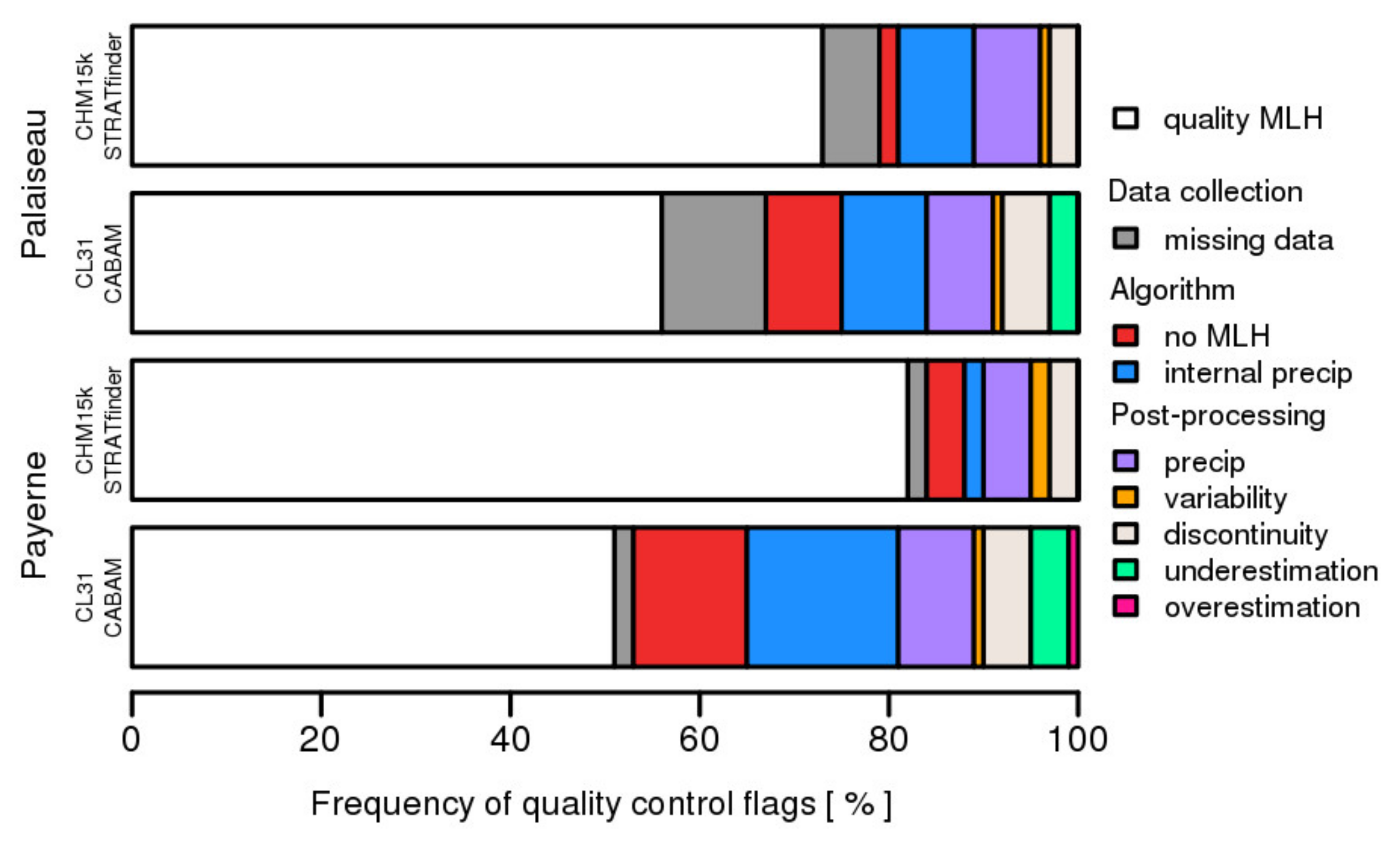
3.1. Detection Rates and Quality Control

High data availability (attenuated backscatter at Payerne (Palaiseau) observed 98% (89–94%) of the time) allowed for MLH detection to be performed on large datasets. After all quality control flags are applied (Figure 2), more MLH results are available from STRATfinder (82% at Payerne, 73% at Palaiseau) compared to CABAM (51% at Payerne, 56% at Palaiseau). Of these, MLH is detected by both algorithms simultaneously 44% (46%) of the time at Payerne (Palaiseau). Data availability by season and time of day at both sites are sufficient for analysis (37–54%;

Table 2. Data availability [%] of periods when both CABAM and STRATfinder results pass quality control at the two sites, stratified by season and time of day with NT (night-time: sunset + 2 h until sunrise), MO (morning: sunrise until sunrise + 4 h), DT (daytime: sunrise + 4 h until sunset − 2 h), and EV (evening: sunset − 2 h until sunset + 2 h).

	Payerne					Palaiseau
	All	NT	MO	DT	EV	All	NT	MO	DT	EV
Winter	44	53	46	47	39	48	53	48	53	45
Spring	41	45	38	42	41	47	48	42	53	47
Summer	43	38	37	49	38	47	45	43	52	51
Autumn	49	54	45	49	49	43	47	40	47	40

).

In a few complex cases (2% at both sites), no layer was detected by STRATfinder. CABAM does not assume a continuous layer throughout the day so that layer heights may be interrupted when no significant gradient is present in the attenuated backscatter profile at a consistent height. These layer gaps and insufficient SNR explain the higher data fraction, with no MLH detected by the low-SNR ALC (12% at Payerne, 8% at Palaiseau). At Payerne, CABAM flags more periods with complex precipitation patterns (16%) compared to STRATfinder (2%), while the internal precipitation flag is more consistent between algorithms (7–9%) at Palaiseau. Further refinement of the respective modules implemented for detection of precipitation could help increase agreement of this quality flag between algorithms. Still, the internal precipitation flag is preferable to simply excluding time periods based on auxiliary precipitation measurements because such data may not always be available, and commonly used systems (such as tipping buckets) do not capture the complexity of precipitation affecting the attenuated backscatter profiles. During post-processing quality control (Section 2.3), about the same amount of data (5–8%) are further excluded due to precipitation for results from the two algorithms.

Few periods are excluded due to unrealistic layer height variability below 300 m for both methods at both sites (1–2%). CABAM results are slightly more often discarded due to unrealistic temporal discontinuity (5% at both sites) compared to STRATfinder (3%). Additional 3–4% (~1%) of CABAM results are flagged for daytime underestimation (nocturnal overestimation).

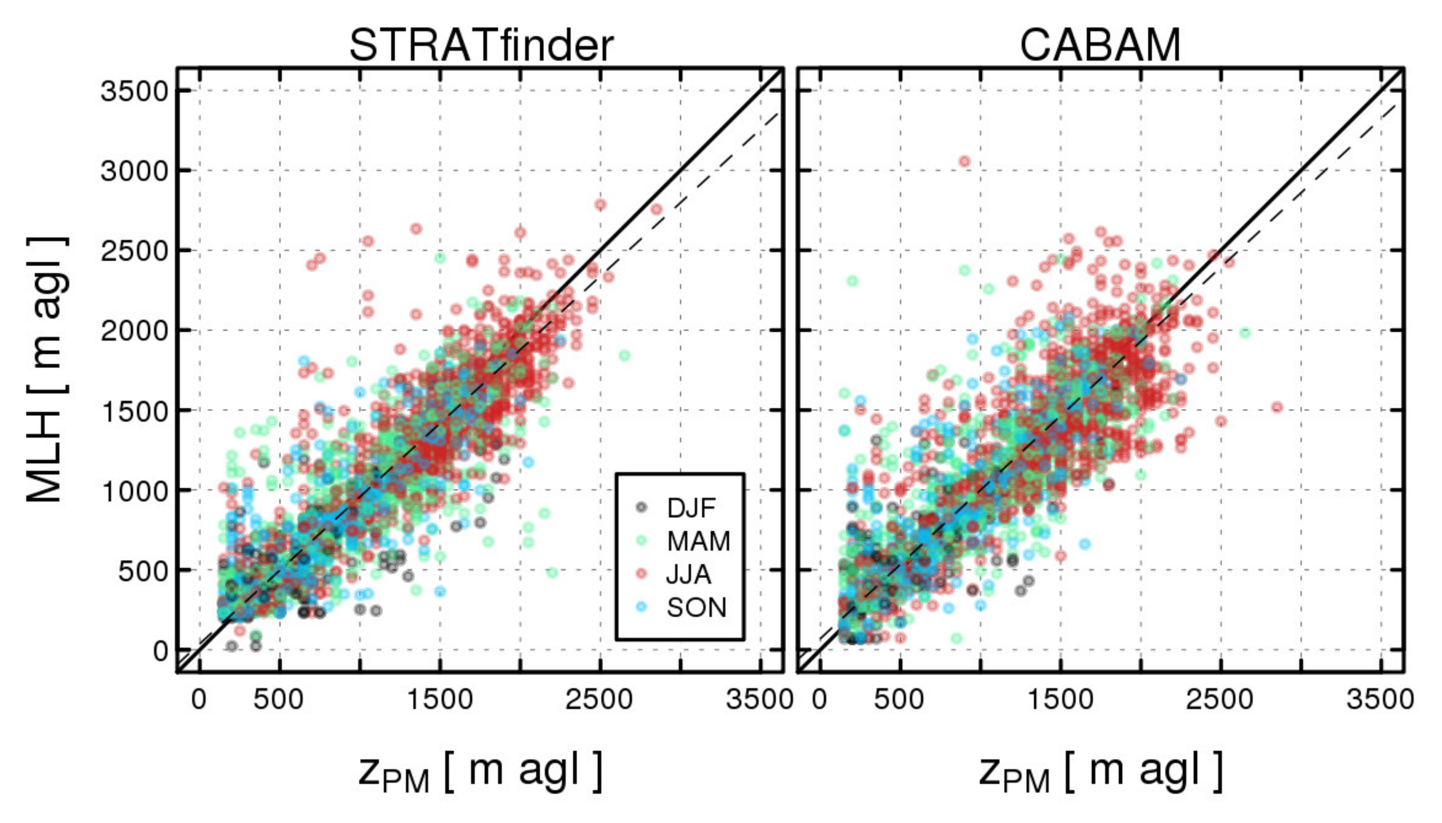
3.2. Evaluation against Thermodynamic Boundary Layer Height

The Palaiseau MLH from STRATfinder and CABAM are evaluated using thermodynamic layer heights derived for the Paris region based on temperature profiles collected by AMDAR (Section 2.4). The high density of reporting airplanes permitted the parcel method height (z_PM) and the height of first temperature inversion (z_ΔT) to be detected 7% and 21% of the time, respectively. Given multi-layer clouds at the top of the ABL are often associated with high temporal variability in the observed temperature profile, days with multi-layer clouds (range of reported CBH between 5 h after sunrise and sunset > 1000 m) or rainfall (diagnosed from ALC) are excluded from analysis. Further, only days are selected when all three methods have data. With most z_PM available in spring and summer, simultaneous layer estimates with the ALC are available for about 2% of the total analysis period.

Overall comparison between the AMDAR layer height z_PM and CABAM and STRATfinder estimates (

Table 3. Comparison between Paris region AMDAR parcel method (z_PM), thermodynamic layer height, and Palaiseau ALC-derived mixed layer height with CABAM and STRATfinder algorithms for times when all three methods are available, stratified by season (DJF: winter, MAM: spring, JJA: summer, SON: autumn). Metrics are: number of samples (N), mean bias error (MBE), mean absolute error (MAE), root mean square error (RMSE), hit rate (HR) with a 300 m absolute deviation threshold, slope (a) and intercept (b) of linear relation, and coefficient of determination (R²).

	STRATfinder					CABAM
	All	DJF	MAM	JJA	SON	All	DJF	MAM	JJA	SON
N	2530	184	836	1136	374	2530	184	836	1136	374
MBE [m]	−54	−69	−52	−63	−26	−10	−16	0	−36	47
MAE [m]	200	207	201	198	198	213	189	203	229	203
RMSE [m]	280	293	291	270	277	303	265	295	317	296
HR [%]	79	77	79	79	79	75	80	77	72	78
a	0.92	0.78	0.88	0.95	0.87	0.93	0.8	0.92	0.94	0.99
b [m]	38	81	78	11	97	70	115	87	43	61
R2	0.75	0.53	0.66	0.77	0.69	0.7	0.59	0.65	0.67	0.67

; Figure 3) indicate the two ALC-based methods have similar statistical agreement. Absolute deviations are slightly smaller for STRATfinder leading to lower MAE and RMSE values and slightly higher hit rates, i.e., overall 79% (75%) of the STRATfinder (CABAM) MLH are within 300 m of the parcel method estimates.

STRATfinder has a small negative bias to z_PM, consistent with other comparisons of thermodynamic layers heights and aerosol-derived MLH [32,39]. CABAM overestimates occur (Figure 3) at times when false layers are detected within the noise region above the ABL as a result of the low SNR signal recorded by the CL31. As the quality control procedure (Section 2.3) is not able to capture all such instances, these over-estimations bring the MBE closer to zero for CABAM (Table 3).

Assessed against AMDAR thermodynamic layer heights, the performance of CABAM at Palaiseau (Table 3) is markedly better than reported for the long-term dataset from London, UK [17]. Improvements of the CABAM MLH by application of the automatic quality control is unlikely responsible for the smaller errors reported here, given supervised layer detection was used in London to minimise false layer attribution. However, z_PM is a more appropriate MLH reference than the temperature inversion height used to evaluate the London MLH, with the latter often marking the top of the residual layer [17]. As synoptic conditions and cloud dynamics modify ABL complexity and sublayer configurations, they may also influence the performance statistics at the two sites.

Comparison of STRATfinder MLH to AMDAR z_PM (Table 3) indicates slightly poorer performance than previous evaluations of its predecessors to radiosonde ascents interpreted with the bulk Richardson method [40]. Estimates at noon for one year at Payerne using pathfinderTURB had a similar MBE (~−50 m) but a RMSE of 162 m (R² = 0.85) [22]. STRAT+ MLH at Palaiseau during spring and summer (5 months) was found to be within ± 150 m of radiosonde layer estimates for 94% of the time (R² = 0.968). The higher discrepancies between STRATfinder and the AMDAR layer estimates could be explained by a combination of different sources of uncertainty:

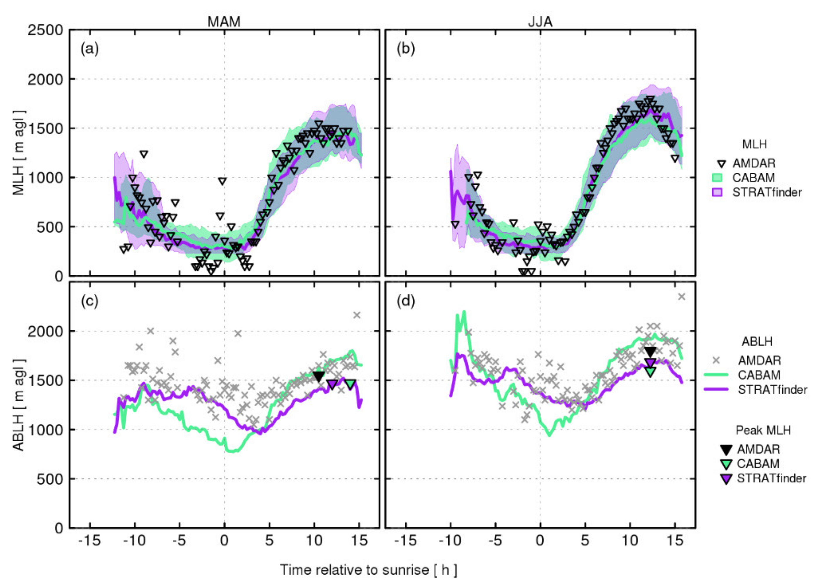
• While previous evaluations against radiosondes were limited to midday conditions (noon ascents), the current AMDAR assessment spans the whole day, including nocturnal periods (Figure 4).
• The mode of data collection for the temperature profile contributes to the uncertainty. While the absolute measurement accuracy of AMDAR data is less than for radiosondes [41], systematic temperature biases are not critical to the ABL layer height detection [34]. However, the vertical resolution of the temperature profiles is usually higher for radiosondes compared to AMDAR. Further, horizontal displacement is greater for airplane flight paths (~10 km km⁻¹, ∆x ∆z⁻¹) than radiosondes (~1 km km⁻¹) [34], which cause changes in both vertical mixing and ABL height when there are variations in orography and/or land-cover [42]. Substantial spatial variations in ABL heights have been found in the Paris area during spring and summer [43].
• Uncertainty arises from thermodynamic retrieval of layer heights from AMDAR and radiosonde profiles. The parcel method and the bulk Richardson method can give different results (e.g., peak MLH at Payerne had MAE of 50–250 m [5]). By selecting only days when these two methods are in “good” agreement (difference < 250 m), Poltera et al. [22] likely removed more complex conditions that lead to a mismatch between aerosol-derived and radiosonde-based MLH estimates. Unfortunately, as the bulk Richardson method requires wind data that are very rarely reported in the AMDAR system, it is not applied here despite being considered better for estimating the convective boundary layer height [5].
• The auxiliary data used by STRAT+ to derive MLH may help reduce uncertainty in aerosol-based layer detection. Further, application to a high-power lidar [15] rather than an ALC likely decreases false layer detection.

Still, the AMDAR dataset provides a beneficial reference for the evaluation the ALC methods as radiosonde ascents [44] do not allow full diurnal evolution of the ABL heights to be assessed.

It is further evaluated how the average seasonal diurnal evolution of the ABL heights compares between the aerosol-based methods and the thermodynamic approach (Figure 4). More simultaneous data are available in spring and summer (Table 3) when unstable atmospheric conditions are more frequent. Here, the MLH is the median z_PM from sunrise + 3 h until sunset, the 10^th percentile of z_ΔT for the night and early morning. The average ABLH is the 75^th percentile of the seasonal z_ΔT statistics.

MLH from both ALC-based methods have a similar diurnal pattern to the AMDAR derived diagnostics (Figure 4a,b). While the AMDAR MLH has considerable uncertainty and temporal variability at night when layers are shallower, the median MLH agrees well during the early morning growth (2–3 h past sunrise). Overall, median AMDAR MLH is within the inter-quartile range of both ALC-derived MLH. In summer, STRATfinder daytime maxima are closer to the AMDAR results (Figure 4b) as the low SNR of the CL31 means periods with deep ABL development are neither always captured accurately by CABAM nor filtered by the quality control (Section 2.3).

The various physical processes related to turbulent mixing and entrainment may result in characteristic vertical profiles of wind, temperature, moisture, and aerosol [45]. Detected layer boundaries differ slightly depending on the method and tracer(s) used. Previous studies found thermodynamic layer heights derived from Doppler wind lidar measurements tend to rise ahead of ALC-based MLH, often reaching greater daytime peak values [31,39]. Layer heights derived from microwave radiometer profiles [5] showed an earlier and faster boundary layer morning growths of results derived based on the bulk Richardson method compared to those from the parcel method. Here, AMDAR MLH starts growing at a similar time as the ALC-derived MLH estimates but then continues to rise at a higher rate to slightly greater heights. Hence, it appears that layer estimates that incorporate wind or turbulence observations tend to detect earlier and faster boundary layer growth compared to methods solely based on temperature and aerosol-based MLH further lag behind the latter.

Given the considerable uncertainty in the ABLH statistics (e.g., substantial temporal variability, Figure 4c,d), only a qualitative first-order comparison of the seasonal average diurnal ABLH based on temperature inversions and ALC is conducted. All three methods indicate an ABLH at a reasonable height above the nocturnal MLH. However, the median diurnal ABLH from the ALC are systematically lower compared to the AMDAR ABLH reference, with a greater underestimation by CABAM (−405 m/−189 m on average in spring/summer) than by STRATfinder (−191 m/−84 m in spring/summer) for the time between sunset and sunrise + 3 h. After this, the AMDAR ABLH mostly falls in-between the CABAM and STRATfinder layer estimates. In autumn and winter (insufficient data for metrics), the temperature inversions are frequently closer to the ABLH results from CABAM.

According to classical ABL theory [45], the mixed layer is expected to extend over the whole ABL following the morning growth period. However, not all methods show the MLH merging into the ABLH (Section 2) during the day on average (Figure 4). While this behaviour is nicely reproduced by ABLH from STRATfinder and AMDAR, CABAM ABLH is strongly overestimated, hence exceeding peak MLH by 512 m (610 m) in spring (summer). This is the first time ABLH is derived in addition to MLH from both AMDAR and ALC observations. Although considerable uncertainty remains for the ABLH derived from low-SNR ALC observations, both AMDAR and ALC analysis have the potential to capture the full ABL sublayer configuration including both the mixed layer and the residual layer. This illustrates the need and benefits of further algorithm development and improved quality control.

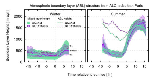
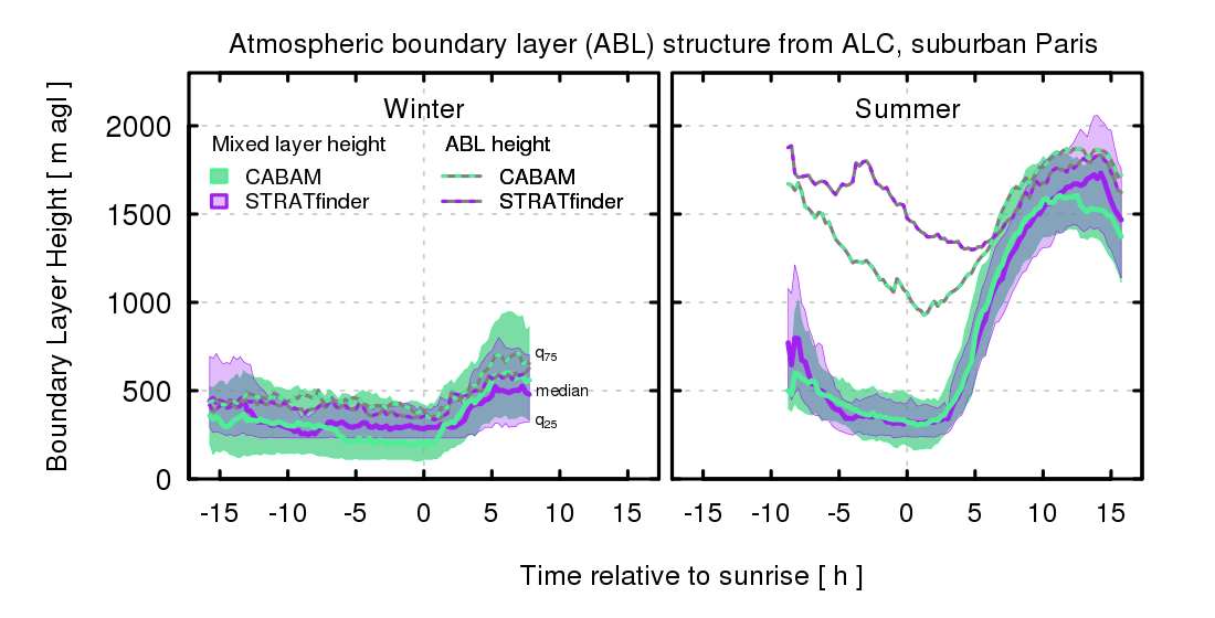
3.3. Average ABL Heights

The STRATfinder and CABAM ability to characterise the ABL heights at the two study sites is assessed. The two independent aerosol-based methods have very similar median diurnal cycle of MLH by season at both Payerne (Figure 5a–d) and Palaiseau (Figure 5e–h). MLH tends to decrease through the night, most evident in the CABAM Palaiseau results. As expected [28,36], MLH starts to rise a few hours after sunrise, with peak values in the afternoon. Median MLH peaks at similar levels at these two sites (Figure 5). The average growth is slightly steadier at Payerne. MLH decreases once there is reduced buoyant activity in the afternoon. In Palaiseau, in spring and summer, this may be hours before sunset, while the height remains rather constant in Payerne. In winter and autumn, at neither site do the two algorithms detect a decay in median MLH before sunset. However, in summer during the evening transition, differences between two ALC types are apparent with the CABAM MLH on average decreasing ahead of the STRATfinder results. These findings should be interpreted with care as the number of data points used to calculate average MLH is considerably lower around sunset (Figure 5) due to changes in solar position over the course of a season. Furthermore, the time of MLH decay is particularly challenging to track using aerosol-based methods as the formation of gradients in attenuated backscatter is likely to depend on aerosol characteristics (e.g., size distributions).

Mostly, the two algorithms capture a very similar behaviour of the nocturnal MLH. However, STRATfinder has slightly larger values at both sites during winter. The very low variability of nocturnal STRATfinder MLH around sunrise in spring and summer at Payerne suggests the algorithm tends to follow the lowest detection limit (Section 2.1) leading to a small average under-estimation compared to CABAM. During morning growth, CABAM MLH occasionally rises ahead of the STRATfinder results, which could be explained by aerosol gradients within or at the top of the residual layer being mistaken for the mixed layer height. This leads to a very small positive bias for CABAM during this time of day.

Overall, the seasonal average MLH from the two ALC have both mean and median differences mostly within ±100 m and very similar diurnal ABL behaviour.

When differentiating between clear and cloudy conditions (not shown), a similar agreement between the average MLH patterns from the two algorithms is found. At both sites, the two algorithms detect greater summer peak MLH on days with convective clouds compared to cloud-free conditions. The effect of a deeper MLH when clouds are forming at the top of the ABL during deep convection is consistent with earlier studies at Palaiseau [36] and London [28].

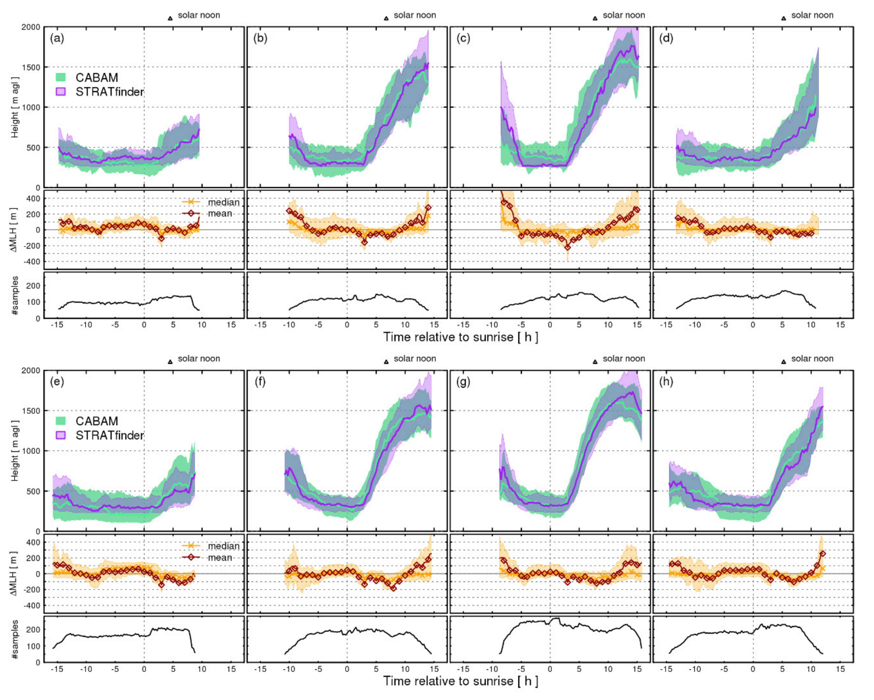
3.4. Direct Comparison of MLH from High-SNR and Low-SNR ALC

Comparison of individual 15 min MLH estimates from STRATfinder and CABAM (

Table 4. Comparison statistics between ALC-based MLH from CABAM and STRATfinder algorithms at Payerne and Palaiseau for all periods and stratified by time of day (see Figure 6 and Table 3 or definitions).

	Payerne					Palaiseau
	All	NT	MO	DT	EV	All	NT	MO	DT	EV
N	45211	17590	8064	12734	6823	72867	29018	13408	19127	11314
MBE [m]	15	8	−55	−13	169	−4	7	−22	−65	96
MAE [m]	214	183	187	215	325	192	175	153	195	277
RMSE [m]	362	281	308	375	539	326	271	256	350	458
a	1.03	0.32	0.38	1.07	1.2	0.95	0.55	0.39	0.92	1.14
b [m]	−5	268	238	−83	14	28	178	226	27	−30
R2	0.53	0.02	0.21	0.56	0.39	0.64	0.07	0.18	0.61	0.5

, Figure 6) confirms the general agreement of the two algorithms at both sites (Section 3.3). Across all data, the linear regression slope is close to unity with a negligible intercept and small MBE. Substantial deviations between MLH from the two methods do occur occasionally (Figure S1) leading to MAE ~200 m and RMSE ~350 m. Still, MLH from the two methods are within 300 m of each other for 77–80% of the time (Figure 6). Given the slightly larger scatter at Payerne, there is marginally better statistical agreement between the methods at Palaiseau. From the summary statistics (Table 4), the aerosol-based MLH determined using the two ALC algorithms are in similar agreement as when either is compared to the thermodynamic layer heights (Section 3.2).

Positive and negative deviations between the STRATfinder and CABAM MLH occur during all periods of the day (Figure 6). At night, the MAE remains below 200 m and the MBE indicates no clear bias between methods. As CABAM’s MLH morning growth is occasionally too rapid (Section 3.3), a small negative bias of STRATfinder is detected for morning (MO) and daytime (DT) periods. When the MLH estimates are particularly similar (< 100 m), CABAM MLH is 6% (10%) more likely to be greater than the STRATfinder-derived layer estimate at Payerne (Palaiseau).

As the CABAM MLH starts to decrease earlier than the STRATfinder MLH (Section 3.3), the MBE is positive and substantial around sunset. During the evening (EV), STRATfinder MLH is 15% (21%) more likely to exceed the corresponding CABAM result by more than 100 m than vice versa at Palaiseau (Payerne). Although a similar number of MLH results from the two algorithms are within 100 m of each other during all periods of the day (Figure 6), the relative deviations are smaller during DT and EV when the absolute magnitude of MLH is greatest. Hence, more MLH values are close to the 1:1 line in the direct comparison (Figure S1) during daytime and evening, leading to an improved linear regression slope and higher coefficient of determination compared to night-time (NT) and MO (Table 4).

The relatively low linear regression slope and coefficient of determination during night and early morning (Table 4) are partly explained by the increased likelihood of STRATfinder MLH being close to its minimum detection height. At night, CABAM frequently has MLH below 200 m at Payerne (Palaiseau) (28% (30%) of the times when both have values). STRATfinder can only detect layers below the minimum detection limit associated with the incomplete optical overlap (Section 2.5) when low clouds or fog are present. As a result, the distributions of MLH at night clearly differ between the two ALC sensor types (Figure 7). Instead of detecting layers below 200 m, STRATfinder assigns layers above 250 m (200 m) at Payerne (Palaiseau). 40% of the nocturnal MLH are between 250–300 m at Payerne as the CHM15k detection limit is higher than for the Palaiseau sensor (Section 2.5). Both algorithms agree nocturnal MLH ≤ 300 m are similarly likely at the two sites (42% at Payerne; 44% at Palaiseau of times when both have data, which is 42% (Payerne) and 45% (Palaiseau) of the possible nocturnal periods).

CABAM nocturnal layer heights have a slightly wider distribution at Palaiseau, but MLH up to ~550 m occur more frequently with the STRATfinder method as its nocturnal search region is restricted by an upper boundary (Section 2.1). Hence, the nocturnal distribution of STRATfinder MLH is sensitive to the user-specified search region. For example, using a search region of 1000 m (cf. 700 m used in the current analysis, Appendix A) creates a positive nocturnal bias (cf. CABAM) at both sites. Note, as the maximum search region also depends on the tracked ABLH (Section 2.1), it is possible for the MLH to exceed the nocturnal maximum specified by the user.

4. Discussion of Site and Sensor Specifics

Applying automatic algorithms to detect the MLH, and potentially ABLH, in a diverse sensor network requires sensor-specific characteristics to be accounted for. The algorithms STRATfinder (Section 2.1) and CABAM (Section 2.2) are designed to take advantage of high-SNR and low-SNR ALC observations, respectively. While discrepancies remain between the methods applied to process observations from the two ALC types (Section 3), their results show very similar seasonal diurnal configurations of the ABL (Section 3.3) and even often agree when individual 15 min values are compared (Section 3.4).

As the algorithms are tested for specific ALC sensors (i.e., Lufft CHM15k [22] for STRATfinder and Vaisala CL31 for CABAM [17]), a first-order assessment of their applicability to other ALC models is performed. For this, STRATfinder is used with Lufft CHM8k data and CABAM with Vaisala CL51 data (Supplementary Materials S.3). Applying the algorithms to the different ALC models is straight forward and without requiring software alterations.

For reference, the CHM15k STRATfinder MLH is used. Both the STRATfinder CHM8k and CABAM CL51 data are affected by the SNR. Given the signal strength of the CHM8k is lower than for the CHM15k (Table 1), uncertainties increase during daytime peak convection, especially when the ABL configuration is complex. Occasionally an overestimation of CHM8k MLH (cf. CHM15k) occurs when the pathfinding algorithm has difficulties distinguishing between the signal in the ABL and either the noise in the free atmosphere, elevated aerosol, or cloud layers aloft. Case studies (Supplementary Materials S.3.1) highlight the importance of absolute calibration of attenuated backscatter [46,47], as this would allow consistent parameter settings across a diverse network. CL51 data are less noisy than CL31 observations (Table 1) leading to slightly better agreement with the STRATfinder CHM15k results (Supplementary Materials S.3.2), even without application of the deep convection module. These first comparisons suggest that the two automatic algorithms are flexible for application in a network setting and further highlight that algorithm performance depends on the quality of the input data provided.

Contrasting SNR characteristics of commonly deployed ALC (CHM15k, CL31) motivated the classification into high- and low-SNR categories. As the low-SNR CL31 does not permit good quality variance fields to be derived, STRATfinder is not suitable to use for this model. However, applying STRATfinder based on CL51 data still needs to be evaluated. Given the CL51 and CHM8k similarities (Table 1), further analysis of long-term measurements with comparison to high-power sensor data could help determine which SNR category is the best fit for these ALC models.

As the choice of site-specific settings (Appendix A) influences the agreement between STRATfinder and CABAM MLH (Section 3), it is important to consider how parameters affect performance by time of day:

(1)

Night: While the STRATfinder MLH search region has an upper limit set, the lower limit is defined by the optical overlap of the individual CHM15k sensor. CABAM can assign any height if there is no other layer below and the layer is temporally consistent. Nocturnal overestimation by CABAM (currently mostly excluded by post-processing quality control) could be reduced if absolute restrictions were implemented, such as for STRATfinder. However, performance in complex cases requires further evaluation. The STRATfinder upper search limit affects the nocturnal MLH distribution, as multiple significant gradients in attenuated backscatter may occur within the residual layer. As STRATfinder does not necessarily follow the layer closest to the ground but rather the stronger negative gradient, elevated layer boundaries within or at the top of the RL may be assigned instead of a weak MLH. Additionally, the instrument optical overlap function is demonstrated (Section 3.4, Figure 7) to impact the detection at very low layer heights. When interpreting MLH results from multiple sensors across a network, this effect must be considered.

(2)

Morning: As STRATfinder uses a pathfinding method, while CABAM connects layers via a decision tree, methodological differences affect their relative performance during morning growth of the mixed layer. CABAM’s rules decide if a layer above or one later in time should be appended to form a consistent MLH estimate. When the MLH rises quickly, the upward turbulent transport of aerosols and entrainment of residual layer air with potentially contrasting characteristics means layer boundaries may not increase in height steadily., MLH can rather suddenly connect to layers existing above and may even alternate up and down (e.g., [48]). While STRATfinder can follow a more complex path, CABAM decisions are simpler, being based on three growth limit values for short-, medium-, and long-distance layer connections (Appendix A). Where rapid, deep convection is common (e.g., Palaiseau), these values need to be set accordingly. Hence, different CABAM settings are used at the two sites in this study. The STRATfinder pathfinding upper boundary is derived from a series of user-defined settings (Section 2.1), including a nocturnal and daytime maximum and a specific growth rate when transitioning between those limits in the morning.

(3)

Daytime: Both methods require a physically possible daytime maximum ABLH to be specified (Appendix A). However, it has minimal impact on performance (unless set too low). During daytime deep convection, a low-SNR sensor is clearly inferior to high-SNR observations. False layers induced by noise may lead to both over- and under-estimation of peak MLH values, depending on the growth limit settings. The improved CABAM performance at Palaiseau with CL51 (cf. CL31) data illustrates this source of uncertainty. The new deep convection module generally improves CABAM performance for CL31 input at Palaiseau where fast growing mixed layers occur frequently during spring and summer. However, occasionally the residual layer may not be completely entrained into the mixed layer during morning growth, or aerosol layers may be advected horizontally without being mixed into the ABL. Such detached, elevated aerosol layers create a very complex ABL that makes MLH tracing even more challenging. On such days, the deep convection module leads to severe MLH overestimation that is not removed by the post-processing quality control. In mountainous Payerne, detached aerosol layers are commonly observed above the ABL [22], so the deep convection module would lead to frequent daytime overestimation and is hence not activated. In addition, activating the deep convection module for MLH detection in an area where the ABL is generally shallower than over Palaiseau [17,28] (e.g., London, UK, where CABAM was developed) could decrease daytime performance.

It has been demonstrated, that the two independent ALC algorithms give comparable MLH estimates. Fully automatic application in a network requires objective methods to specify suitable, site (and potentially sensor) -specific settings. First-order estimates of the general search region limits can be obtained from other ABL methods (e.g., radiosondes) and/or based on the cloud base height climatology given the importance of cloud dynamics to the ABL. Cloud base height data are typically available at ALC sites (prior to recording attenuated backscatter profiles) or can be obtained from other sources (e.g., weather reports). Noise levels of the instrument could be exploited (e.g., to estimate likelihood of false layer detection from low-SNR observations).

5. Conclusions

With increasing density of automatic lidar and ceilometer (ALC) networks the complexity of atmospheric boundary layer (ABL) dynamics that result from the vast heterogeneity of the Earth’s surface and cloud processes will be better captured. This is crucial to provide more detailed information for the evaluation of high-resolution numerical models and potentially aid data assimilation. In July 2020, the European ALC network within the EUMETNET E-PROFILE initiative had 333 ALC across 22 countries [49]. Where land cover or orography are particularly diverse, efforts are being made to further increase sensor density. Reliable, automatic methods are needed to derive higher order products, such as the ABL heights, from this vast amount of data.

Here, two algorithms for automatic detection of the ABL heights are compared to assess their ability to provide consistent information in a heterogeneous ALC network. Commonly used ALC can be roughly divided into (1) relatively high signal-to-noise ratio (SNR) and (2) rather low SNR. The two methods considered are designed to exploit these respective types. STRATfinder, a synthesis of two existing ALC algorithms, is applied for the first time to track the mixed layer height (MLH) and the height of the ABL (ABLH) from high-SNR ALC observations. CABAM, developed for low-SNR ALC to track MLH and additional layers composing the residual layer, is improved and made more flexible for application in a network setting. While both algorithms perform MLH detection at high temporal resolution (≤1 min), 15 min averages are compared.

Measurements from two E-PROFILE network sites with diverse ABL characteristics are used: (1) rural Payerne (Switzerland) has orography that leads to a complex ABL with elevated aerosol layers detached from the ABL and (2) suburban Palaiseau (Paris, France) has frequent rapid deep mixing in spring and summer. Nearly 3 years (Payerne) and 4.5 years (Palaiseau) of simultaneous observations from the two ALC types are analysed.

First the ALC data are processed to E-PROFILE standards to account for sensor specific artefacts and ensure the profile observations are more consistent between instruments. Both algorithms consider the presence of clouds and precipitation to exclude periods when MLH cannot reliably be determined from attenuated backscatter profile observations. Additional filters are applied during post-processing to remove MLH results that appear physically unreasonable (e.g., based on temporal consistency). After quality control, STRATfinder provides more data. At both sites, simultaneous MLH results are available for nearly 50% of the time, with rather homogeneous diurnal and seasonal distribution.

Agreement between the two independent aerosol-based algorithms is similar to when either is compared to thermodynamic layer heights derived from temperature profiles gathered across the Paris region by the Aircraft Meteorological Data Relay (AMDAR; [32]). AMDAR parcel method derived heights are slightly greater than ALC MLH in the morning growth period. This suggests the boundary layer height growth differs with the tracer analysed: faster growth occurs if variations in wind or turbulence are analysed, compared to layer heights solely diagnosed from temperature profiles, which again grow slightly faster than aerosol-based layer estimates. ALC results and AMDAR statistics converge during the day to very similar peak layer heights. MLH from the different methods are within 300 m of each other for about 80% of the time.

Average seasonal diurnal patterns of the ABL described by MLH from STRATfinder and CABAM are very similar, both for cloudy and cloud-free conditions. The greatest discrepancy occurs during the evening decay of the mixed layer around sunset, when STRATfinder has a delayed decline of the mixed layer (cf. CABAM). The MLH decay is challenging to track using aerosol-based information as the gradients in attenuated backscatter likely depend on aerosol characteristics (e.g., size distributions).

With a low-SNR ALC, layer detection uncertainty increases when MLH rises fast to high peak levels (above 2000 m), as instrument-related noise can cause gradients in attenuated backscatter within the mixed layer that may be falsely assigned to the MLH. The new deep convection module improves performance for such spring and summer days at Palaiseau, but it occasionally leads to over-estimation when detached elevated aerosol layers occur above the ABL.

Correlation between MLH from the ALC methods is lower at night and early morning (cf. day-time when the mixed layer is well-established). While layers as low as 50 m can be derived by CABAM with the low-SNR ALC, the high-SNR ALC is poorer at detecting shallow layers because of its incomplete optical overlap. As the optical overlap function is instrument-specific the respective instrument’s blind zone (here below 250 m at Payerne, below 200 m at Palaiseau) affects the distribution of shallow layer heights detected. At both sites the algorithms agree on the probability of nocturnal MLH to be below 300 m (42–44% of times when both have data available). Further do STRATfinder user settings affect the distribution of nocturnal layer results and consequently the agreement between the ALC methods during this time.

First-order estimates of total ABLH are compared, with AMDAR and STRATfinder having reasonable agreement in spring and summer. Both confirm the textbook expectation of the mixed layer extending over the whole ABL once full daytime development is reached. CABAM’s ABLH is significantly overestimated during the day suggesting a dedicated module to track ABLH is needed. Results demonstrate the full ABL sublayer configuration can be characterised automatically solely based on ALC observations provided careful data analyses and quality control. Being able to analyse not only the mixed layer but also the evolution of the residual layer has distinct advantages for interpreting air quality measurements and modelling.

The present analysis shows very good agreement between the MLH from high- and low-SNR ALC can be achieved at two sites with differing ABL dynamics. Careful selection of site-specific parameters generally improves algorithm performance. To apply the automatic ABL methods across a wider range of stations within a diverse network, general criteria are needed to objectively determine appropriate settings. This could use cloud base height statistics. The absolute calibration of recorded ALC signal into units of attenuated backscatter is essential for generic thresholds to be specified. With attenuated backscatter routinely calibrated and corrected for instrument-specific artefacts, objective site-specific settings will allow high-quality products of ABL heights to be possible at national and continental scale.

References

- Mittermaier, M.P. A Strategy for Verifying Near-Convection-Resolving Model Forecasts at Observing Sites. Weather Forecast. 2014, 29, 185–204. [Google Scholar] [CrossRef]
- Illingworth, A.J.; Cimini, D.; Haefele, A.; Haeffelin, M.; Hervo, M.; Kotthaus, S.; Löhnert, U.; Martinet, P.; Mattis, I.; O’Connor, E.J.; et al. How Can Existing Ground-Based Profiling Instruments Improve European Weather Forecasts? Bull. Am. Meteorol. Soc. 2019, 100, 605–619. [Google Scholar] [CrossRef]
- Cazorla, A.; Casquero-Vera, J.A.; Román, R.; Guerrero-Rascado, J.L.; Toledano, C.; Cachorro, V.E.; Orza, J.A.G.; Cancillo, M.L.; Serrano, A.; Titos, G.; et al. Near-real-time processing of a ceilometer network assisted with sun-photometer data: Monitoring a dust outbreak over the Iberian Peninsula. Atmos. Chem. Phys. 2017, 17, 11861–11876. [Google Scholar] [CrossRef]
- Collaud Coen, M.; Praz, C.; Haefele, A.; Ruffieux, D.; Kaufmann, P.; Calpini, B. Determination and climatology of the planetary boundary layer height above the Swiss plateau by in situ and remote sensing measurements as well as by the COSMO-2 model. Atmos. Chem. Phys. 2014, 14, 13205–13221. [Google Scholar] [CrossRef]
- Dang, R.; Yang, Y.; Hu, X.-M.; Wang, Z.; Zhang, S. A Review of Techniques for Diagnosing the Atmospheric Boundary Layer Height (ABLH) Using Aerosol Lidar Data. Remote Sens. 2019, 11, 1590. [Google Scholar] [CrossRef]
- Shi, Z.; Vu, T.; Kotthaus, S.; Harrison, R.M.; Grimmond, S.; Yue, S.; Zhu, T.; Lee, J.; Han, Y.; Demuzere, M.; et al. Introduction to the special issue “In-depth study of air pollution sources and processes within Beijing and its surrounding region (APHH-Beijing)”. Atmos. Chem. Phys. 2019, 19, 7519–7546. [Google Scholar] [CrossRef]
- Stirnberg, R.; Cermak, J.; Kotthaus, S.; Haeffelin, M.; Andersen, H.; Fuchs, J.; Kim, M.; Petit, J.; Favez, O. Meteorology-driven variability of air pollution ( PM1 ) revealed with explainable machine learning. Atmos. Chem. Phys. Discuss. 2020, 1–35. [Google Scholar] [CrossRef]
- Klein, A.; Ancellet, G.; Ravetta, F.; Thomas, J.L.; Pazmino, A. Characterizing the seasonal cycle and vertical structure of ozone in Paris, France using four years of ground based LIDAR measurements in the lowermost troposphere. Atmos. Environ. 2017, 167, 603–615. [Google Scholar] [CrossRef]
- Banks, R.F.; Tiana-Alsina, J.; Rocadenbosch, F.; Baldasano, J.M. Performance Evaluation of the Boundary-Layer Height from Lidar and the Weather Research and Forecasting Model at an Urban Coastal Site in the North-East Iberian Peninsula. Bound. -Layer Meteorol. 2015, 157, 265–292. [Google Scholar] [CrossRef]
- Ciais, P.; Dolman, A.J.; Bombelli, A.; Duren, R.; Peregon, A.; Rayner, P.J.; Miller, C.; Gobron, N.; Kinderman, G.; Marland, G.; et al. Current systematic carbon-cycle observations and the need for implementing a policy-relevant carbon observing system. Biogeosciences 2014, 11, 3547–3602. [Google Scholar] [CrossRef]
- Lauvaux, T.; Miles, N.L.; Deng, A.; Richardson, S.J.; Cambaliza, M.O.; Davis, K.J.; Gaudet, B.; Gurney, K.R.; Huang, J.; O’Keefe, D.; et al. High-resolution atmospheric inversion of urban CO2 emissions during the dormant season of the Indianapolis Flux Experiment (INFLUX). J. Geophys. Res. Atmos. 2016, 121, 5213–5236. [Google Scholar] [CrossRef] [PubMed]
- Geiß, A.; Wiegner, M.; Bonn, B.; Schäfer, K.; Forkel, R.; von Schneidemesser, E.; Münkel, C.; Chan, K.L.; Nothard, R. Mixing layer height as an indicator for urban air quality? Atmos. Meas. Tech. 2017, 10, 2969–2988. [Google Scholar] [CrossRef]
- de Bruine, M.; Apituley, A.; Donovan, D.P.; Klein Baltink, H.; de Haij, M.J. Pathfinder: Applying graph theory to consistent tracking of daytime mixed layer height with backscatter lidar. Atmos. Meas. Tech. Discuss. 2017, 10, 1893–1909. [Google Scholar] [CrossRef]
- Morille, Y.; Haeffelin, M.; Drobinski, P.; Pelon, J. STRAT: An Automated Algorithm to Retrieve the Vertical Structure of the Atmosphere from Single-Channel Lidar Data. J. Atmos. Ocean. Technol. 2007, 24, 761–775. [Google Scholar] [CrossRef]
- Pal, S.; Haeffelin, M.; Batchvarova, E. Exploring a geophysical process-based attribution technique for the determination of the atmospheric boundary layer depth using aerosol lidar and near-surface meteorological measurements. J. Geophys. Res. Atmos. 2013, 118, 9277–9295. [Google Scholar] [CrossRef]
- Haeffelin, M.; Angelini, F.; Morille, Y.; Martucci, G.; Frey, S.; Gobbi, G.P.; Lolli, S.; O’Dowd, C.D.; Sauvage, L.; Xueref-Rémy, I.; et al. Evaluation of Mixing-Height Retrievals from Automatic Profiling Lidars and Ceilometers in View of Future Integrated Networks in Europe. Bound. Layer Meteorol. 2012, 143, 49–75. [Google Scholar] [CrossRef]
- Kotthaus, S.; Grimmond, C.S.B. Atmospheric Boundary Layer Characteristics from Ceilometer measurements Part 1: A new method to track mixed layer height and classify clouds. Q. J. R. Meteorol. Soc. 2018, 144, 1525–1538. [Google Scholar] [CrossRef]
- Martucci, G.; Matthey, R.; Mitev, V.; Richner, H. Frequency of Boundary-Layer-Top Fluctuations in Convective and Stable Conditions Using Laser Remote Sensing. Bound. -Layer Meteorol. 2010, 135, 313–331. [Google Scholar] [CrossRef]
- Di Giuseppe, F.; Riccio, A.; Caporaso, L.; Bonafé, G.; Gobbi, G.P.; Angelini, F. Automatic detection of atmospheric boundary layer height using ceilometer backscatter data assisted by a boundary layer model. Q. J. R. Meteorol. Soc. 2012, 138, 649–663. [Google Scholar] [CrossRef]
- Gan, C.-M.; Wu, Y.; Madhavan, B.L.; Gross, B.; Moshary, F. Application of active optical sensors to probe the vertical structure of the urban boundary layer and assess anomalies in air quality model PM2.5 forecasts. Atmos. Environ. 2011, 45, 6613–6621. [Google Scholar] [CrossRef]
- Wang, Z.; Cao, X.; Zhang, L.; Notholt, J.; Zhou, B.; Liu, R.; Zhang, B. Lidar measurement of planetary boundary layer height and comparison with microwave profiling radiometer observation. Atmos. Meas. Tech. 2012, 5, 1965–1972. [Google Scholar] [CrossRef]
- Poltera, Y.; Martucci, G.; Collaud Coen, M.; Hervo, M.; Emmenegger, L.; Henne, S.; Brunner, D.; Haefele, A. PathfinderTURB: An automatic boundary layer algorithm. Development, validation and application to study the impact on in situ measurements at the Jungfraujoch. Atmos. Chem. Phys. 2017, 17, 10051–10070. [Google Scholar] [CrossRef]
- Wiegner, M.; Mattis, I.; Pattantyús-Ábrahám, M.; Bravo-Aranda, J.A.; Poltera, Y.; Haefele, A.; Hervo, M.; Görsdorf, U.; Leinweber, R.; Gasteiger, J.; et al. Aerosol backscatter profiles from ceilometers: Validation of water vapor correction in the framework of CeiLinEx2015. Atmos. Meas. Tech. 2019, 12, 471–490. [Google Scholar] [CrossRef]
- Kotthaus, S.; O’Connor, E.; Münkel, C.; Charlton-Perez, C.; Haeffelin, M.; Gabey, A.M.; Grimmond, C.S.B. Recommendations for processing atmospheric attenuated backscatter profiles from Vaisala CL31 ceilometers. Atmos. Meas. Tech. 2016, 9, 3769–3791. [Google Scholar] [CrossRef]
- Hervo, M.; Poltera, Y.; Haefele, A. An empirical method to correct for temperature-dependent variations in the overlap function of CHM15k ceilometers. Atmos. Meas. Tech. 2016, 9, 2947–2959. [Google Scholar] [CrossRef]
- Wiegner, M.; Madonna, F.; Binietoglou, I.; Forkel, R.; Gasteiger, J.; Geiß, A.; Pappalardo, G.; Schäfer, K.; Thomas, W. What is the benefit of ceilometers for aerosol remote sensing? An answer from EARLINET. Atmos. Meas. Tech. 2014, 7, 1979–1997. [Google Scholar] [CrossRef]
- E-PROFILE. Available online: http://eumetnet.eu/activities/observations-programme/current-activities/e-profile/ (accessed on 30 August 2020).
- Kotthaus, S.; Grimmond, C.S.B. Atmospheric Boundary Layer Characteristics from Ceilometer measurements, Part 2: Application to London’s Urban Boundary Layer. Q. J. R. Meteorol. Soc. 2018, 144, 1511–1524. [Google Scholar] [CrossRef]
- Dijkstra, E.W. A note on two problems in connexion with graphs. Numer. Math. 1959, 1, 269–271. [Google Scholar] [CrossRef]
- Vienna R Foundation for Statistical Computing. R Core Team. R: A Language and Environment for Statistical Computing. 2020. Available online: https://www.R-project.org/ (accessed on 30 August 2020).
- Kotthaus, S.; Halios, C.H.; Barlow, J.F.; Grimmond, C.S.B. Volume for pollution dispersion: London’s atmospheric boundary layer during ClearfLo observed with two ground-based lidar types. Atmos. Environ. 2018, 190, 401–414. [Google Scholar] [CrossRef]
- Met Office. AMDAR (Aircraft Meteorological Data Relay) Reports Collected by the Met Office MetDB System. NCAS British Atmospheric Data Centre. 2008. Available online: http://catalogue.ceda.ac.uk/uuid/220a65615218d5c9cc9e4785a3234bd0 (accessed on 10 July 2020).
- Holzworth, G.C. Estimates of mean and maximum mixing depths in the contiguous United States. Mon. Weather Rev. 1964, 92, 235–242. [Google Scholar] [CrossRef]
- Rahn, D.A.; Mitchell, C.J. Diurnal Climatology of the Boundary Layer in Southern California Using AMDAR Temperature and Wind Profiles. J. Appl. Meteorol. Climatol. 2016, 55, 1123–1137. [Google Scholar] [CrossRef]
- Haeffelin, M.; Barthès, L.; Bock, O.; Boitel, C.; Bony, S.; Bouniol, D.; Chepfer, H.; Chiriaco, M.; Cuesta, J.; Delanoë, J.; et al. SIRTA, a ground-based atmospheric observatory for cloud and aerosol research. Ann. Geophys. 2005, 23, 253–275. [Google Scholar] [CrossRef]
- Pal, S.; Haeffelin, M. Forcing mechanisms governing diurnal, seasonal, and interannual variability in the boundary layer depths: Five years of continuous lidar observations over a suburban site near Paris. J. Geophys. Res. 2015, 120, 11936–11956. [Google Scholar] [CrossRef]
- Heese, B.; Flentje, H.; Althausen, D.; Ansmann, A.; Frey, S. Ceilometer lidar comparison: Backscatter coefficient retrieval and signal-to-noise ratio determination. Atmos. Meas. Tech. 2010, 3, 1763–1770. [Google Scholar] [CrossRef]
- Corripio, J.G. Insol: Solar Radiation. R Package Version 1.1.1. 2014. Available online: https://CRAN.R-project.org/package=insol (accessed on 10 July 2020).
- Barlow, J.F.; Dunbar, T.M.; Nemitz, E.G.; Wood, C.R.; Gallagher, M.W.; Davies, F.; O’Connor, E.; Harrison, R.M. Boundary layer dynamics over London, UK, as observed using Doppler lidar during REPARTEE-II. Atmos. Chem. Phys. 2011, 11, 2111–2125. [Google Scholar] [CrossRef]
- Richardson, L.F. The Supply of Energy from and to Atmospheric Eddies. Proc. R. Soc. Lond. Ser. A Contain. Pap. Math. Phys. Character 1920, 97, 354–373. [Google Scholar] [CrossRef]
- Ballish, B.A.; Kumar, V.K.; Ballish, B.A.; Kumar, V.K. Systematic Differences in Aircraft and Radiosonde Temperatures. Bull. Am. Meteorol. Soc. 2008, 89, 1689–1708. [Google Scholar] [CrossRef]
- Teuling, A.J.; Taylor, C.M.; Meirink, J.F.; Melsen, L.A.; Miralles, D.G.; van Heerwaarden, C.C.; Vautard, R.; Stegehuis, A.I.; Nabuurs, G.-J.; de Arellano, J.V.-G. Observational evidence for cloud cover enhancement over western European forests. Nat. Commun. 2017, 8, 14065. [Google Scholar] [CrossRef]
- Theeuwes, N.E.; Barlow, J.F.; Teuling, A.J.; Grimmond, C.S.B.; Kotthaus, S. Persistent cloud cover over mega-cities linked to surface heat release. NPJ Clim. Atmos. Sci. 2019, 2, 1–15. [Google Scholar] [CrossRef]
- Seibert, P. Review and intercomparison of operational methods for the determination of the mixing height. Atmos. Environ. 2000, 34, 1001–1027. [Google Scholar] [CrossRef]
- Stull, R.B. An Introduction to Boundary Layer Meteorology; Kluwer Acad. Publisher: Dordrecht, The Netherlands, 1988; p. 688. [Google Scholar]
- Wiegner, M.; Geiß, A. Aerosol profiling with the Jenoptik ceilometer CHM15kx. Atmos. Meas. Tech. 2012, 5, 1953–1964. [Google Scholar] [CrossRef]
- Hopkin, E.; Illingworth, A.J.; Charlton-Perez, C.; Westbrook, C.D.; Ballard, S. A robust automated technique for operational calibration of ceilometers using the integrated backscatter from totally attenuating liquid clouds. Atmos. Meas. Tech. 2019, 12, 4131–4147. [Google Scholar] [CrossRef]
- Träumner, K.; Kottmeier, C.; Corsmeier, U.; Wieser, A. Convective Boundary-Layer Entrainment: Short Review and Progress using Doppler Lidar. Bound. -Layer Meteorol. 2011, 141, 369–391. [Google Scholar] [CrossRef]
- Bircher-Adrot, S.; E-PROFILE Team. E-PROFILE ALC Network Monthly Report: July 2020; p. 59. Available online: ftp://ftp.meteoswiss.ch/Monthly_Report/ALC_monitoring_202007.pdf (accessed on 20 August 2020).