An Integrated Geologic Map of the Rembrandt Basin, on Mercury, as a Starting Point for Stratigraphic Analysis

Abstract

Planetary geologic maps are usually carried out following a morpho-stratigraphic approach where morphology is the dominant character guiding the remote sensing image interpretation. On the other hand, on Earth a more comprehensive stratigraphic approach is preferred, using lithology, overlapping relationship, genetic source, and ages as the main discriminants among the different geologic units. In this work we produced two different geologic maps of the Rembrandt basin of Mercury, following the morpho-stratigraphic methods and symbology adopted by many authors while mapping quadrangles on Mercury, and an integrated geo-stratigraphic approach, where geologic units were distinguished also on the basis of their false colors (derived by multispectral image data of the NASA MESSENGER mission), subsurface stratigraphic position (inferred by crater excavation) and model ages. We distinguished two different resurfacing events within the Rembrandt basin, after the impact event, and four other smooth plains units outside the basin itself. This provided the basis to estimate thicknesses, volumes, and ages of the smooth plains inside the basin. Results from thickness estimates obtained using different methodologies confirm the presence of two distinct volcanic events inside the Rembrandt basin, with a total thickness ranging between 1–1.5 km. Furthermore, model ages suggest that the volcanic infilling of the Rembrandt basin is among the ones that extended well into the mid-Calorian period, when Mercury’s effusive volcanism was previously thought to be largely over.

1. Introduction

Geologic maps of other planets are mainly based on units that are distinguished by surface geomorphology (relief, texture) and stratigraphic relations [1], and only secondarily by their color variation. Colors are however indicative of the diverse composition of each unit and/or their different grade of weathering, which in turn is related to their exposure ages. Hence, by ignoring or under-evaluating color variation, geologic mappers are inherently neglecting an important source of information. Such information can improve understanding of the genesis and relative emplacement age of the different geologic units. In this regard, planetary geologic maps are different from classical terrestrial ones, where many other kinds of information apart from geomorphology and texture are taken into consideration.

The surface of Mercury, in particular, is well suited for carrying out mapping where color variations and color derived stratigraphy can be considered to be discriminant factors among geologic units. Throughout Mercury’s history, it has been shaped by impacts and volcanic resurfacing events [2,3,4,5,6,7,8,9,10], giving rise to a complex stratigraphy reflected by an outstanding color variegation on specific red, green and blue (RGB) color composites and a considerable variability in terms of surface composition [11,12,13,14,15,16].

Geologic maps of some quadrangles on Mercury [17,18,19,20] provide the most detailed cartographic products available for the planet up to date. These maps focus on geologic units distinguished mainly on the basis of their morphology, texture (i.e., roughness) and crosscutting relationships with faults, but their stratigraphic relationship has been just barely defined by means of color variegation. Nonetheless, some authors identified stratigraphic correlations across Mercury’s surface also based on spectral characteristics and model ages of geologic units [4,12,21,22,23], where ages are basically assessed through the accumulated numbers of impact craters. Therefore, an integrated approach to planetary mapping, which takes into account both morphology and colors, is highly recommended and provides and essential starting point for further stratigraphic correlation and analysis.

We chose the 715-km diameter Rembrandt basin as one of the most representative areas of Mercury’s stratigraphic variation (Figure 1), displaying a variety of different stratigraphic units, with different ages. The Rembrandt basin is almost coeval with the Caloris basin, with an age bound at 3.8 ± 0.1 Ga [24,25]. The floor of Rembrandt is covered by younger smooth plains (associated with lava infill) that are thought to have been emplaced up to 3.6 ± 0.1 Ga [25], therefore temporally unrelated to the impact event and thus attributed to a volcanic origin [3,24,26]. Furthermore, several spectrally distinct smooth plains cover a large area surrounding the basin, attributed by [26] to either volcanic resurfacing events or impact melt, due to the basin-related impact event. [25] dated the south-western portion of these external plains as coeval with those inside the basin (i.e., 3.6 ± 0.1 Ga), suggesting a possible correlation between the external and the internal events. The western portion of the basin is crosscut by a ~1000-km-long lobate scarp, Enterprise Rupes, which is the longest lobate scarp on Mercury, attributed mainly to crustal shortening induced by global contraction [27], and possibly with a contribution from mantle convection and tidal de-spinning [28,29,30]. The activity of the Enterprise system was dated by [31] between 3.8 ± 0.8 Ga and 2.0 ± 0.4 Ga.

We mapped this area both in a traditional way (morpho-stratigraphic map) and taking into account the surface color variation and stratigraphy (geo-stratigraphic map). Based on the second mapping approach, we also calculated the thickness of the units infilling the Rembrandt basin and estimated their age through crater-counting techniques. Furthermore, we compared the stratigraphic columns of the two maps displaying the age and geologic correlation between the two. Finally, we estimated the volume of the volcanic infilling of the Rembrandt basin.

2. Geologic Mapping Materials and Methods

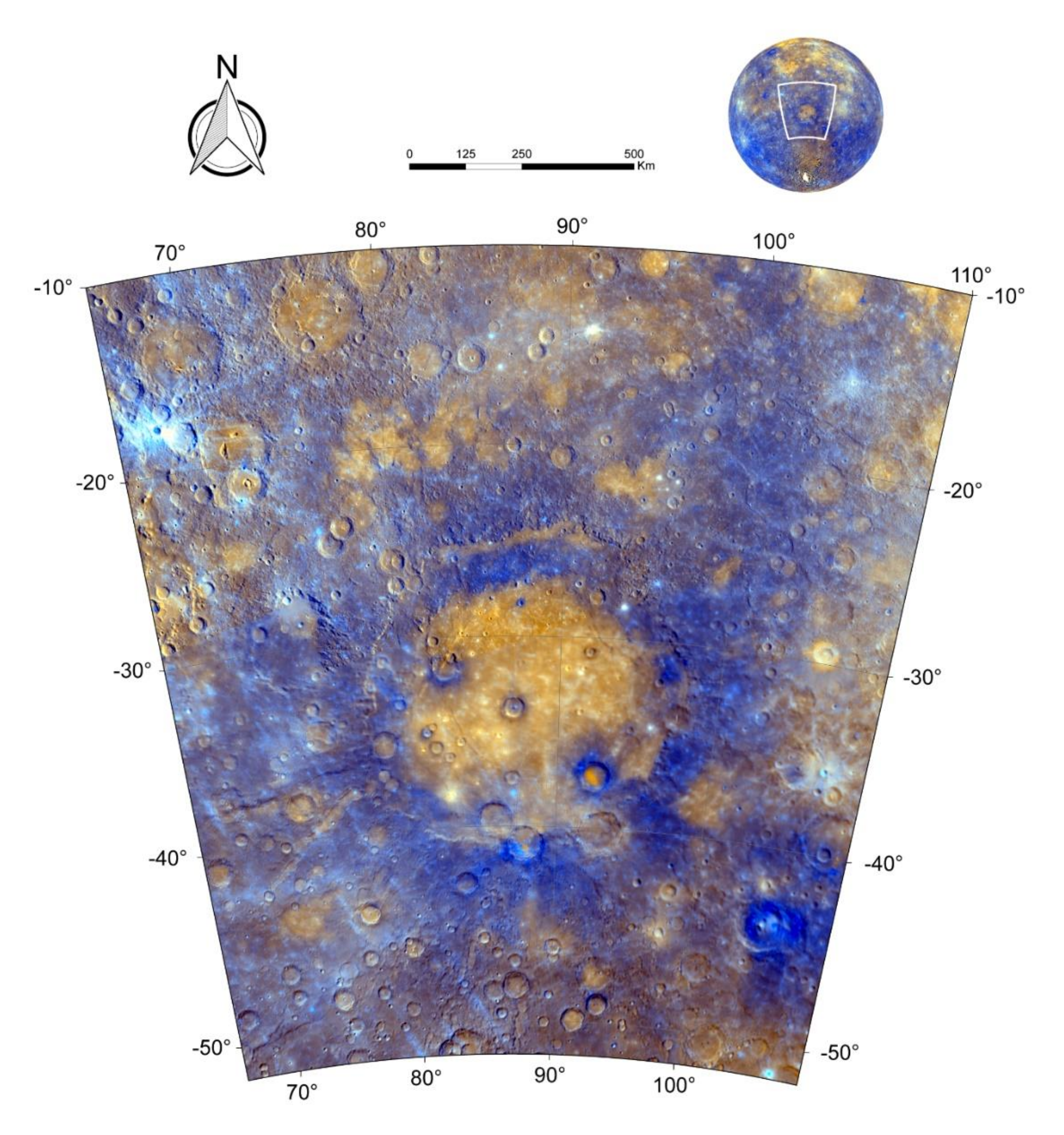
2.1. Data

We used the basemaps derived from the Mercury Dual Imaging System (MDIS) [32], consisting of a wide-angle camera (WAC) and a narrow-angle camera (NAC). A detailed list of the basemaps (last update 12/05/2017) is shown in

Table 1. List of all the basemaps used in this work, including topography.

Basemap	Resolution (m/pixel)	Source
MDIS Global monochrome BDR (map-projected Basemap Reduced Data Record) (v1)	166	https://astrogeology.usgs.gov/search/map/Mercury/Messenger/Global/Mercury_MESSENGER_MDIS_Basemap_BDR_Mosaic_Global_166m
MDIS BDR (v2) (quadrants H09, H10, H13, H14)	166	https://pdsimage2.wr.usgs.gov/Missions/MESSENGER/
MDIS Basemap Low-incidence angle—LOI Global Mosaic	166	https://astrogeology.usgs.gov/search/map/Mercury/Messenger/Global/Mercury_MESSENGER_MDIS_Basemap_LOI_Mosaic_Global_166m
MDIS High-incidence angle East—HIE (v2) (quadrants H09, H10, H13, H14)	166	https://pdsimage2.wr.usgs.gov/Missions/MESSENGER/
MDIS High-incidence angle West—HIW (v2) (quadrants H09, H10, H13, H14)	166	https://pdsimage2.wr.usgs.gov/Missions/MESSENGER/
MDIS Basemap Enhanced-Color Global Mosaic	665	https://astrogeology.usgs.gov/search/map/Mercury/Messenger/Global/Mercury_MESSENGER_MDIS_Basemap_EnhancedColor_Mosaic_Global_665m
MDIS Basemap MD2–Color Global Mosaic	665	https://astrogeology.usgs.gov/search/map/Mercury/Messenger/Global/Mercury_MESSENGER_MDIS_Basemap_MD3Color_Mosaic_Global_665m
MDIS Basemap MDR 8-Color Global Mosaic	665	http://messenger.jhuapl.edu/Explore/Images.html#global-mosaics
For topography: MESSENGER Global DEM (v2)	665	https://astrogeology.usgs.gov/search/map/Mercury/Topography/MESSENGER/Mercury_Messenger_USGS_DEM_Global_665m_v2

, including the global stereo-topography [33].

Monochrome basemaps (166 m/pixel) are based on NAC or WAC 750-nm images. Concerning the 11 available WAC filters, the 2–color mosaic (665 m/pixel) is made up of 1000-nm, 750-nm, and 430-nm RGBs, whereas the Enhanced-Color Global Mosaic (665 m/pixel) (Figure 1) is obtained by placing the second principal component, the first principal component, and the 430 nm/1000 nm ratio in the red, green, and blue channels respectively [3]. The second principal component (red channel) removes most of the maturity effects highlighted by the first principal component (green channel) [3]. Therefore, red-orange materials are interpreted to have different compositions with respect to blue materials, and cyan and green features highlight fresh (less mature) materials. In this regard, false-color mosaics provide information on either compositional differences or on the different degree of weathering, or both [3,12].

2.2. Geographic Coordinate System and Projections

The projection used for mapping areas at mid-latitudes is the Lambert Conformal Conic (LCC) projection, with standard parallels chosen (according to a standard rule) at a distance of 1/6 and 5/6 of the latitudinal range in which the target is included [34]. The center of the Rembrandt basin is at 32.89°S latitude and 87.86°E longitude, so we adopted 26.0°S and 40.0°S as standard parallels and 87.0°E as central meridian. This permitted us to minimize distortions across the mapping area. We used a sphere of 2439.4 km radius as a reference datum to stay consistent with the end-of-mission basemaps geographic reference system [9].

2.3. The Choice of Two Map Layers

In Earth science, geologic maps are often defined according to the different aspects they want to emphasize, so that a geomorphologic map is obviously different from a geo-structural map, and both of them are different from a geo-stratigraphic map or a map of the metamorphic domains.

In planetary sciences ‘morpho-stratigraphic’ maps, assembled on the basis of morphological characteristics and stratigraphic information, are instead considered the standard approach [1] as well as reference base of the official quadrangles [35]. From the Apollo era onward, planetary ‘geologic’ mapping has been carried out on panchromatic and monochromatic images (e.g., see [36,37,38]). However, in recent decades, false-color composites and ancillary compositional data would have given the possibility to attempt a more comprehensive geologic mapping on particularly variegated planetary surfaces such as that of Mercury. It is nonetheless worth remarking that no single-layer map can encompass all the geologic information derivable from a given planetary surface. Therefore, it is logical that in planetary sciences, as on Earth, such integrated stratigraphic maps should be complementary to the morpho-stratigraphic ones.

In this work, we produced two geologic map layers. The first one (‘morpho-stratigraphic’ map) is focused on geomorphology and morpho-stratigraphy and follows the methods and symbology adopted by [17,18,19,20] while mapping Mercury’s quadrangles. The second layer is based on units that can be related to different events and that are also distinguished by their color variegation and model ages. We labelled this map as ‘geo-stratigraphic’, being a more comprehensive geologic mapping with respect to the standard morpho-stratigraphic approach. Therefore, geologic boundaries are drawn following different principles.

In the geo-stratigraphic map layer, the geologic contacts were interpreted following boundaries highlighted by color variations, which did not always coincide with the morphological boundaries. Those that do coincide include the boundaries between smooth plains and more heavily cratered units, fresh ejecta deposits overlapping older units, or well-defined central peak structures emerging from crater floors. Contacts that do not coincide with morphological boundaries include, for instance, stratigraphic boundaries between smooth plains of different colors both inside and outside the Rembrandt basin.

Furthermore, crater materials, including ejecta deposits and central peaks, were mapped and classified taking into consideration their color [12] and their regional stratigraphic position inferred by the crater excavation. Consequently, all the ejecta deposits and central peaks were attributed to the main geo-stratigraphic unit that they originated from, and distinguished from the related autochthonous unit. Furthermore, crater floors were considered to be a separate unit when interpreted as volcanic infill or impact melt, being spectrally distinct and/or without any obvious connections with the surrounding material. In this case, the principle is similar to the geologic maps of volcanic fields on Earth where diverse eruptive complexes are well distinguished from one another.

On both maps we also included all secondary features (i.e., linear and surface features, such as tectonic features, crater-rim crests, secondary crater chains, ejecta rays, hollows material, and probable pyroclastic deposits). Among them, the tectonic features were subdivided into three separate groups, respectively associated with Enterprise Rupes, the Rembrandt-related extensional and contraction features, and all other tectonic features mapped outside the basin.

2.4. Mapping Scale

During the mapping activities we adopted different scales depending on the average resolution of the basemaps used. In particular, we used the cartographic rule set by [39] (see also [35]), according to which the mapping scale should be 2000 times the basemap resolution. While producing the morpho-stratigraphic map, we mapped at a scale varying between 1:300,000 and 1:500,000, based on the resolution of ~166m/pixel of the monochrome basemaps. On the other hand, the geo-stratigraphic map was compiled using false-color basemaps that have spatial resolution of 665 m/pixel, suggesting a mapping scale of more than 1:1,300,000.

To assist the lower scale mapping, we increased false-color basemap resolution using pan-sharpening techniques (e.g., [40,41]). Specifically, we used the Color Normalized (Brovey) Sharpening method (run in the Harris Geospatial ENVI software environment), which multiplied each value of the RGB bands of the 665-m/pixel image by a ratio of the 166-m/pixel monochrome basemaps divided by the sum of the color bands. RGB bands were resampled to 166-m/pixel using the bilinear interpolation algorithm, which allows the conservation of the shapes of surface features [42,43].

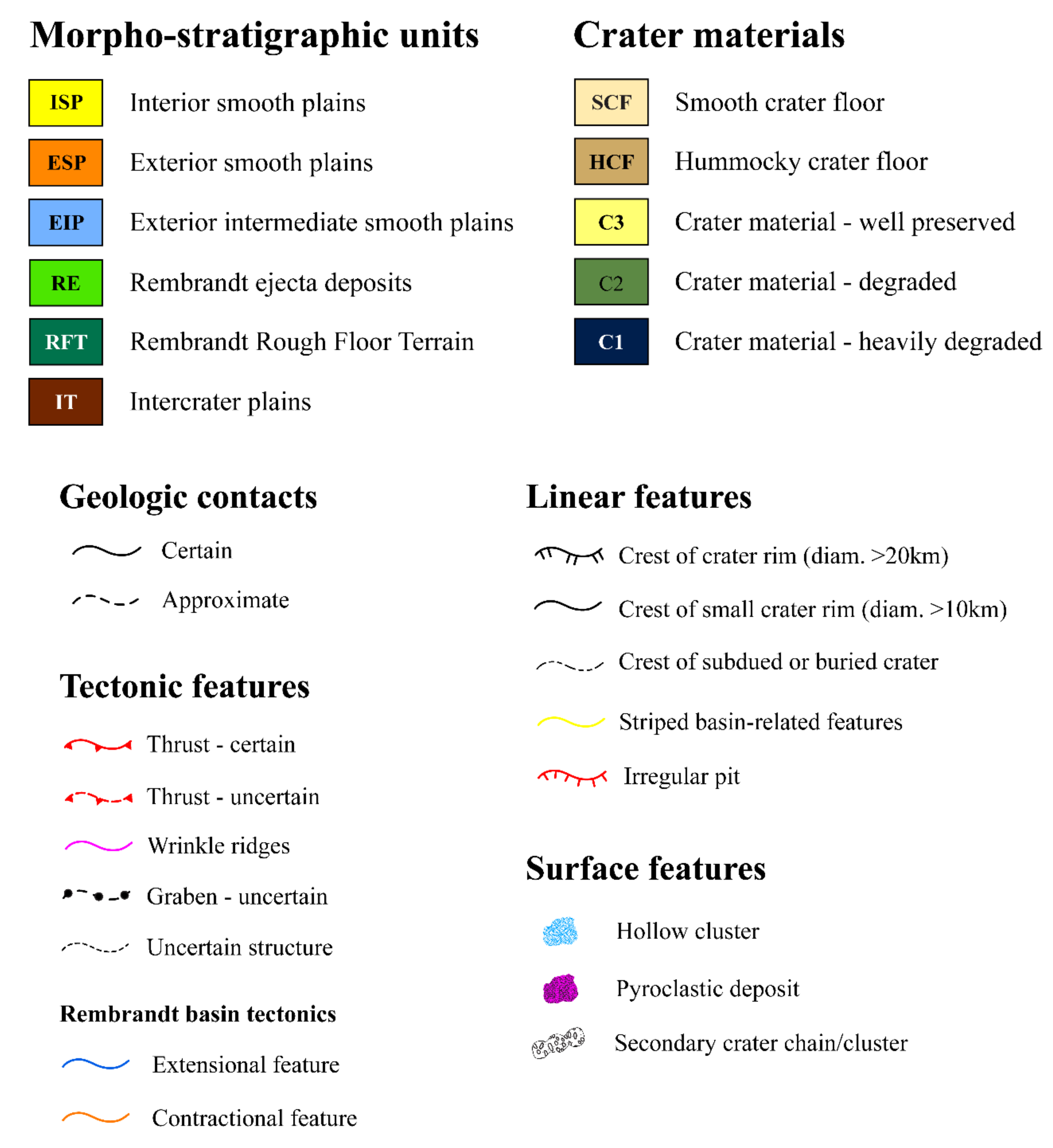
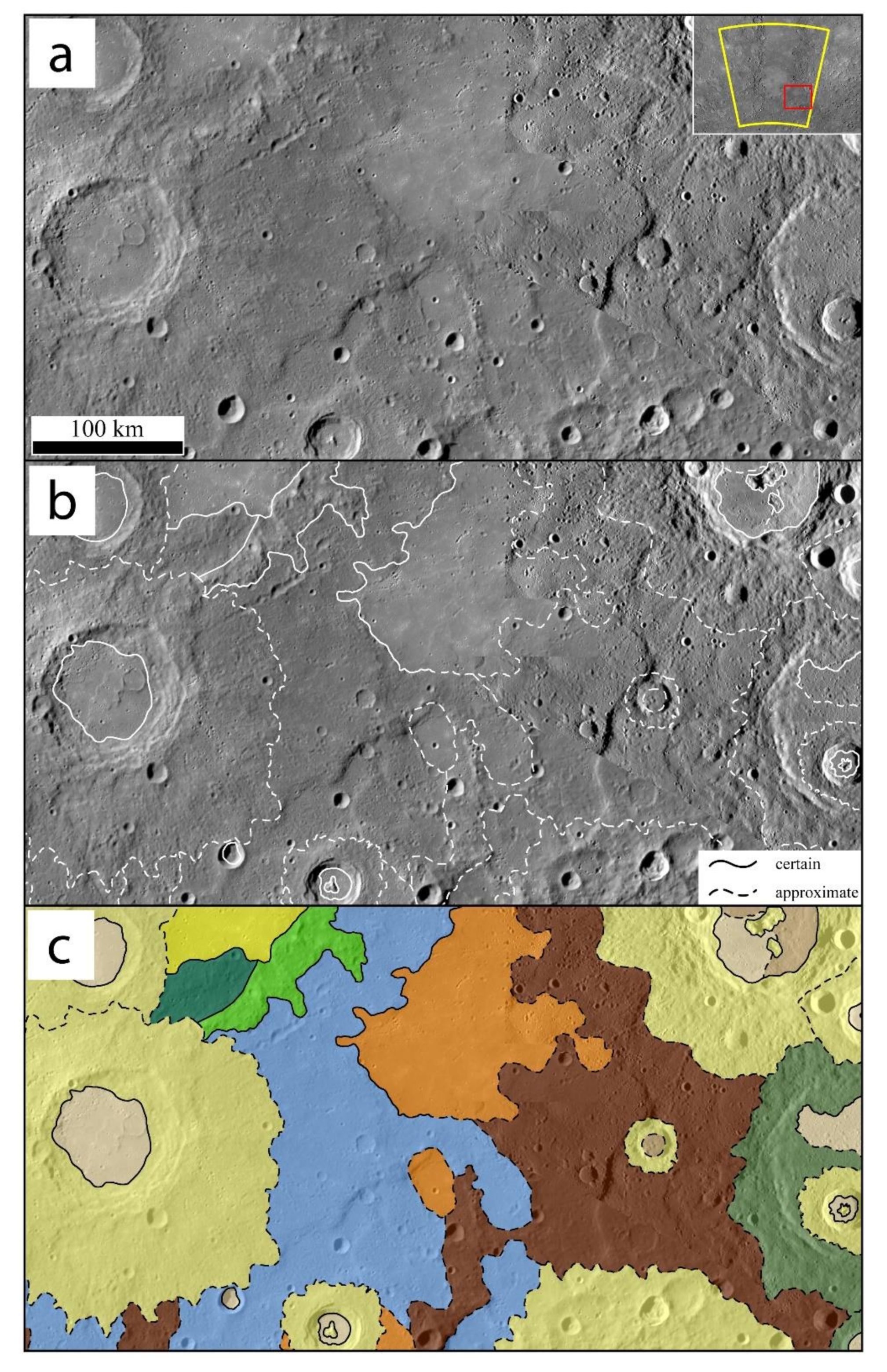
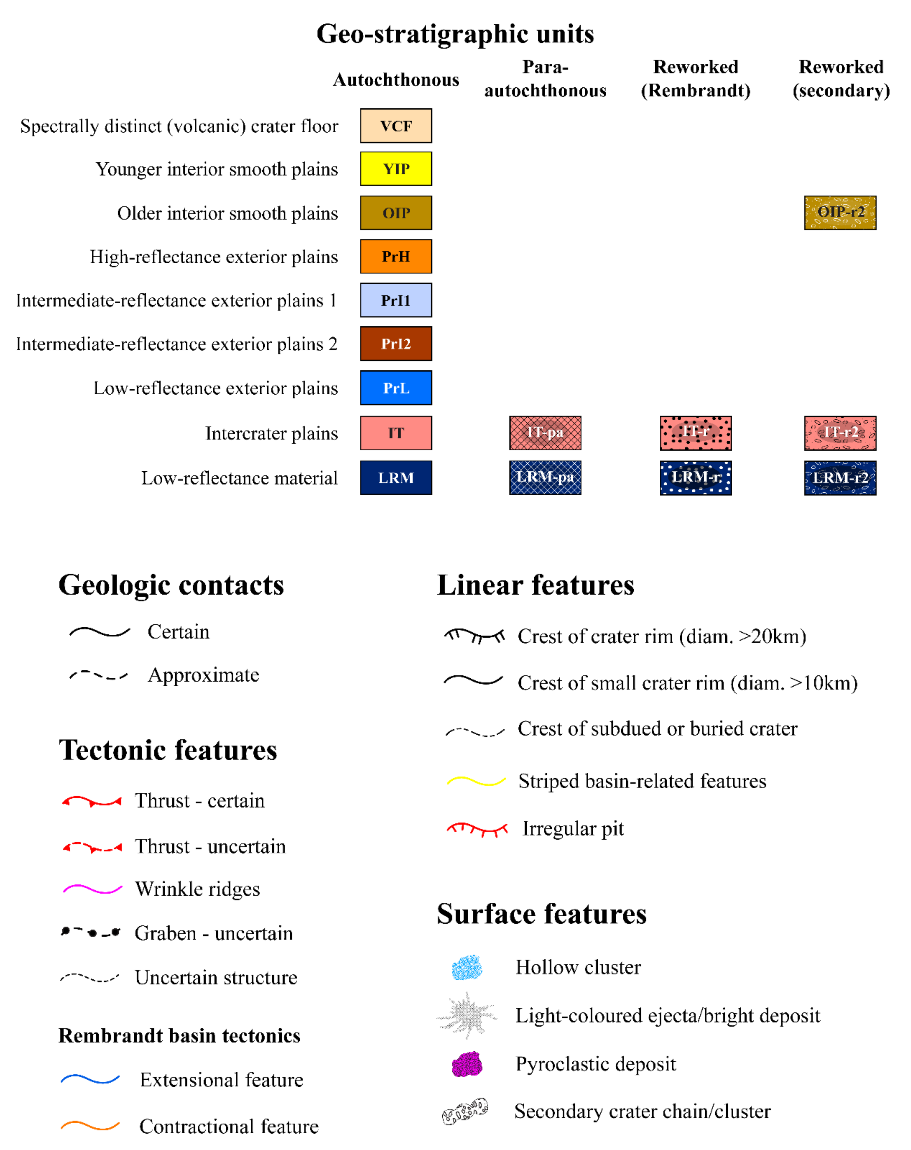
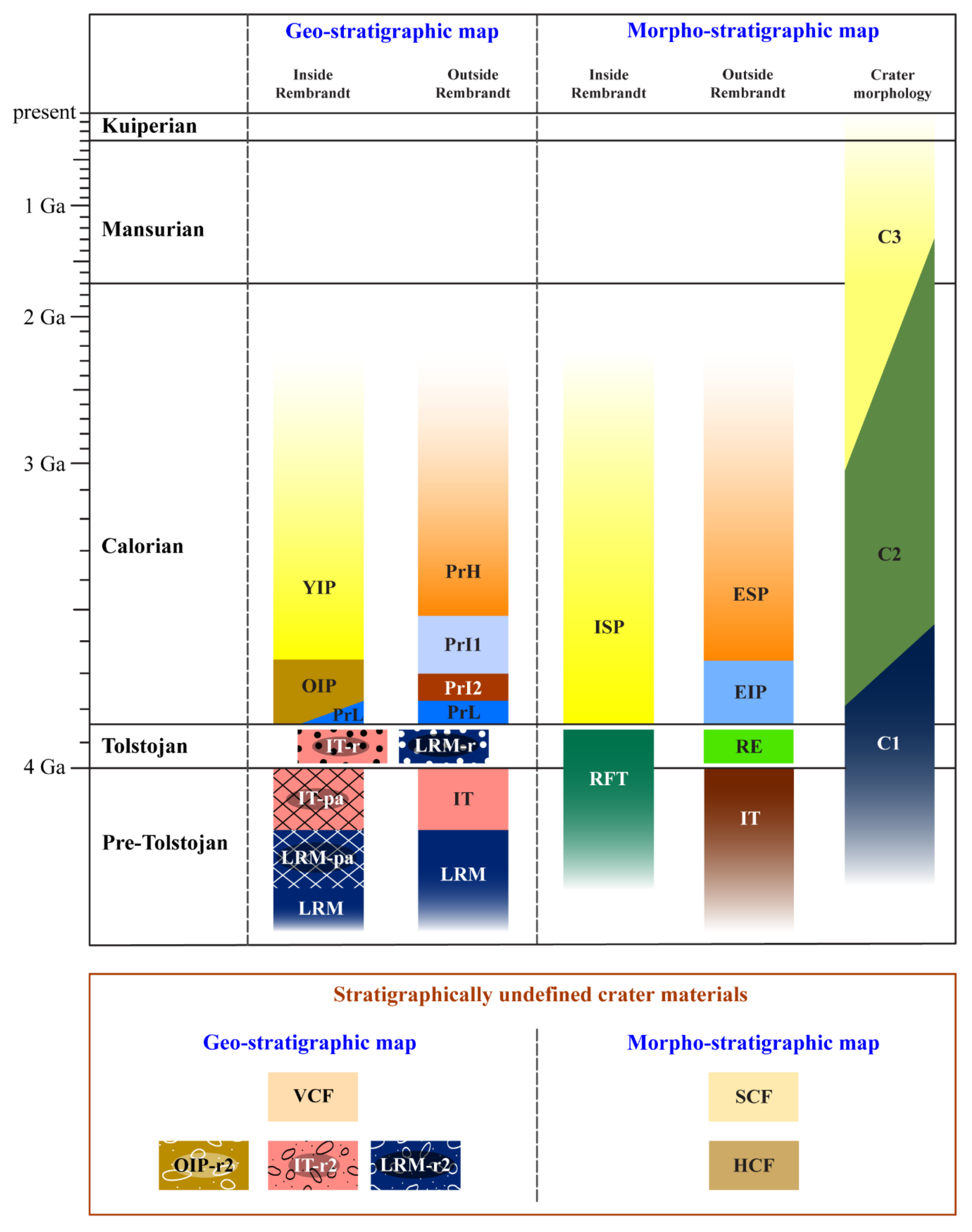
3. Geologic Units Description

In the following sections we describe the main geologic units that we distinguished within the Rembrandt basin and the surrounding area, first based on conventional morpho-stratigraphy, and then by using the geo-stratigraphic approach. The mapping shapefiles and the GIS project of both maps (compatible with the ESRI ArcGIS software) are available in the Supplementary Materials.

The two maps are obviously different and cannot be integrated into a single layer, but being both related to the sequence of geologic events recorded on overlapping units of different relative ages, some relations exist among their units. These relations are discussed comparing their stratigraphic columns in Section 5.

3.1. Morpho-Stratigraphic Map Units

In this section we present the morpho-stratigraphic map and its related units (Figure 2). A detail of the map units is presented in Figure 3.

3.1.1. Interior Smooth Plains (ISP)

These plains are smoother than the surroundings and have higher albedo than the other basin-related units. Interior smooth plains are found in two discontinuous exposures, with no connection to each other. The most extensive part is located in the central portion of the basin, easily distinguishable from the Rembrandt Rough Floor Terrain (RFT—see in the next paragraphs) by its texture; locally it also embays hills of RFT giving a transitional contact with the latter. At their southern boundaries, the ISP appear reworked by superposed craters and are often embayed by ejecta deposits of fresh and younger craters. A less extensive area of interior smooth plains occurs close to the northern basin rim wall. This occurrence is at a higher elevation than the central portion, from which it is separated by the arcuate belt of exposed RFT. The two occurrences are possibly connected through a narrow channel at the western end of the northern example. Due to their similar morphologic properties and continuity, we decided to map all the smooth plains inside the basin as a single morpho-stratigraphic unit.

Like the exterior smooth plains, the ISP display many buried craters, seen as both partially embayed craters and ghost craters, indicating volcanic resurfacing sufficiently long after the basin-forming impact event for the basin floor to have become scarred by subsequent impacts [25]. This is in marked contrast to the Caloris basin, where no embayed or ghost craters are recognized in its interior smooth plains [17].

Additionally, this unit is widely deformed by concentric and radial extensional faults (grabens) and wrinkle ridges, by thrusts and by the Enterprise Rupes system, indicating that its tectonic activity postdates (or at least continued after) the emplacement of these interior smooth plains [25,26,44].

3.1.2. Exterior Smooth Plains

The exterior smooth plains were initially distinguished by [26] into two different units. Following only a morphological classification we were also able to distinguish two smooth plains outside the basin, quite similar to those identified by [26], but with slightly different boundaries (see the detail in Figure 3).

1.

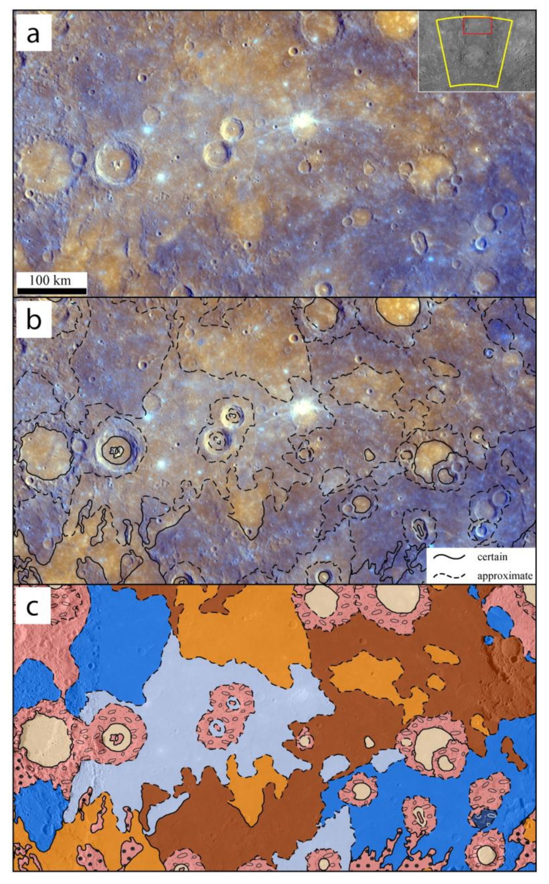
Exterior Smooth Plains (ESP). These plains appear as a smooth, lightly cratered terrain, also distinctly brighter than the surrounding material, and must have been emplaced subsequently to the basin formation (if prior, they would have been destroyed or covered by impact ejecta). As for the ISP, ESP are most probably of volcanic origin [26], showing lower crater density than their surroundings, with which they have sharp morphological boundaries. Furthermore, ESP seem to be controlled by topography, as they mainly occur in topographic lows. They are also modified by post-emplacement tectonics (wrinkle ridges).

2.

Exterior Intermediate Smooth Plains (EIP). These plains display a more cratered terrain and have a slightly rougher texture than all other smooth plains. They do not seem to be confined to topographic lows; instead, each deposit covers both low and high-standing topography. Additionally, EIP are modified by tectonic processes (both wrinkle ridges and lobate scarps), indicating post-emplacement modification. Due to their controversial morphological characteristics, the origin of these plains is still debated, as they could be either volcanic (similarly to the ESP) or impact melt [26].

3.1.3. Rembrandt Ejecta Deposits (RE)

The basin ejecta material is presumed to have formed instantaneously after the impact event and the basin formation. It is found beyond the partially subdued basin rim as a radially lineated terrain that surrounds almost the entire rim crest. It appears as a coherent material, coeval with the rough terrain found inside the basin [25], which is our RFT (see below). Analyzing the area surrounding the Rembrandt basin, some of the basin-related ejecta deposits are found even far away from the basin as closely spaced strips, with sharp morphological boundaries (thus easily recognizable) when overlapping intercrater plains (IT—see below). Therefore, these features can be associated with distal ejecta of the Rembrandt basin, similarly to the Caloris basin [45], and they are often embayed by younger smooth plains. We included the basin-related proximal and distal ejecta within the same unit, since the boundary between the two is often not well-identified.

3.1.4. Rembrandt Rough Floor Terrain (RFT)

This material is composed of a mixture presumed to be impact melt and ejecta deposits (breccias) (see description of the “Hummocky Material” unit in [25]). This unit appears as an undulating and rough terrain that forms hills and depressions. Rougher and lower in albedo than the interior plains, the RFT unit emerges in a concentric arc in the northern half of the basin, but we infer that it underlies the Interior Smooth Plains (ISP) across the whole of the basin. We recognize some smaller patches of exposed RFT within the interior plains in some southern parts of the basin.

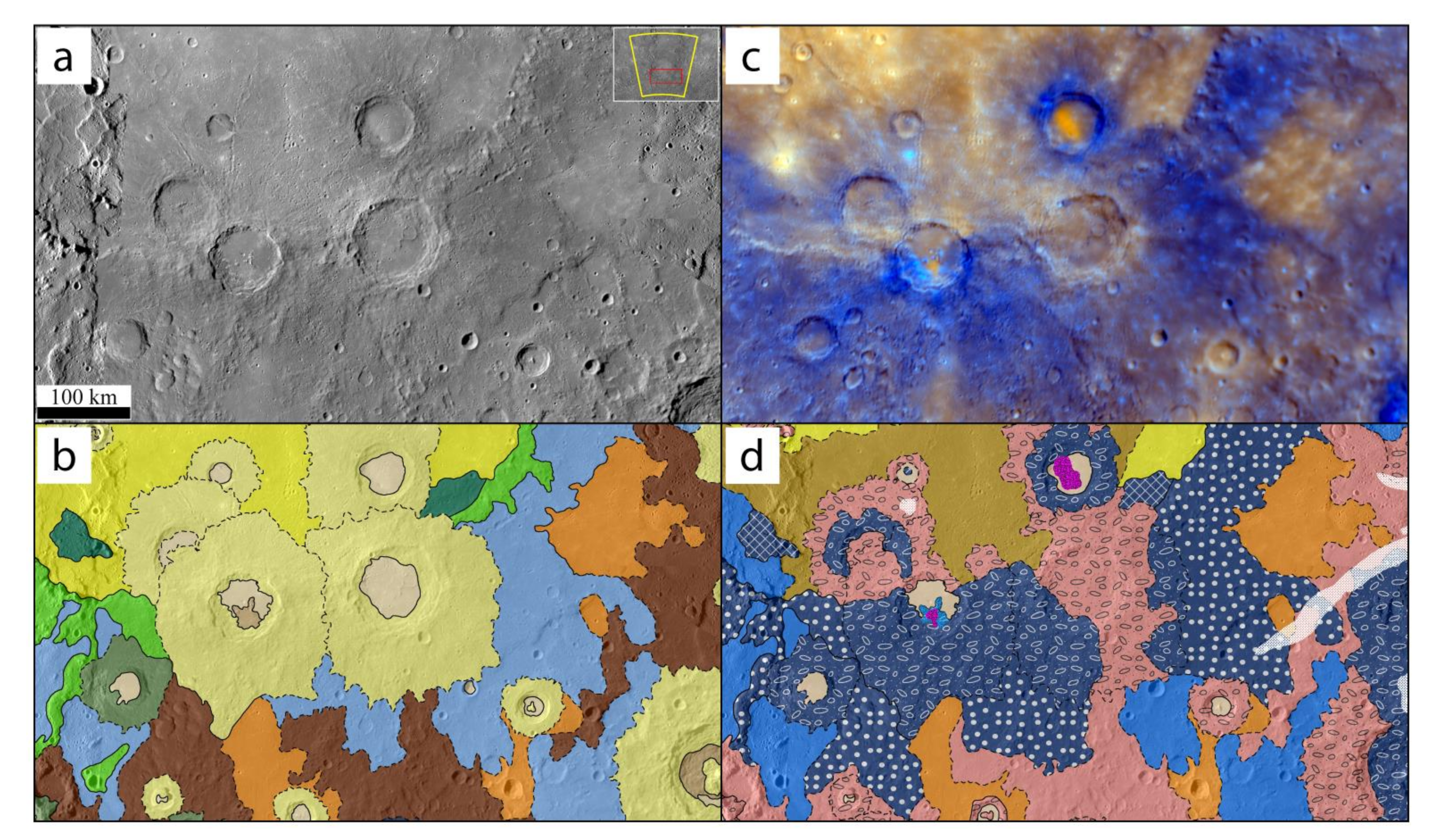
3.1.5. Intercrater Plains (IT)

These plains are the roughest and most cratered surfaces found on our target area, heavily modified by post-emplacement tectonism (see the detail in Figure 3). [46] first recognized, described and mapped this terrain unit as “level to gently rolling ground between and around large craters and basins”. As for the EIP, the origin and identification of these plains has been debated by many authors [2,26,46,47,48,49,50,51] and is not further investigated in our work.

3.1.6. Crater Material

We distinguished three classes of craters, C1–C3, based on their degradation and thus relative age, following the classification proposed by [18] and also adopted by [17,19,20]. This classification represents a simplification compared to the global five-class distinction suggested by [52] and subsequently revised by [53,54]. However, because of the geologic complexity of our study area, we opted for the three-class crater distinction. In particular, C1 and C3 craters are associated respectively to the end members of the oldest and younger craters described by [54] (respectively class 1 and class 5), whereas C2 craters include all other intermediate cases (for further details on this classification, see [18]).

We mapped crater materials for all craters with a diameter > 20 km. Furthermore, we classified the crater floor materials into:

• Smooth crater floor (SCF): smooth crater infill consistent with either impact melt or post-impact volcanism and confined within the crater. They have similar texture compared to that of the smooth plains (interior and exterior).
• Hummocky crater floor (HCF): rough crater infill, including all material reworked during the impact. Very similar texture to that of the IT.

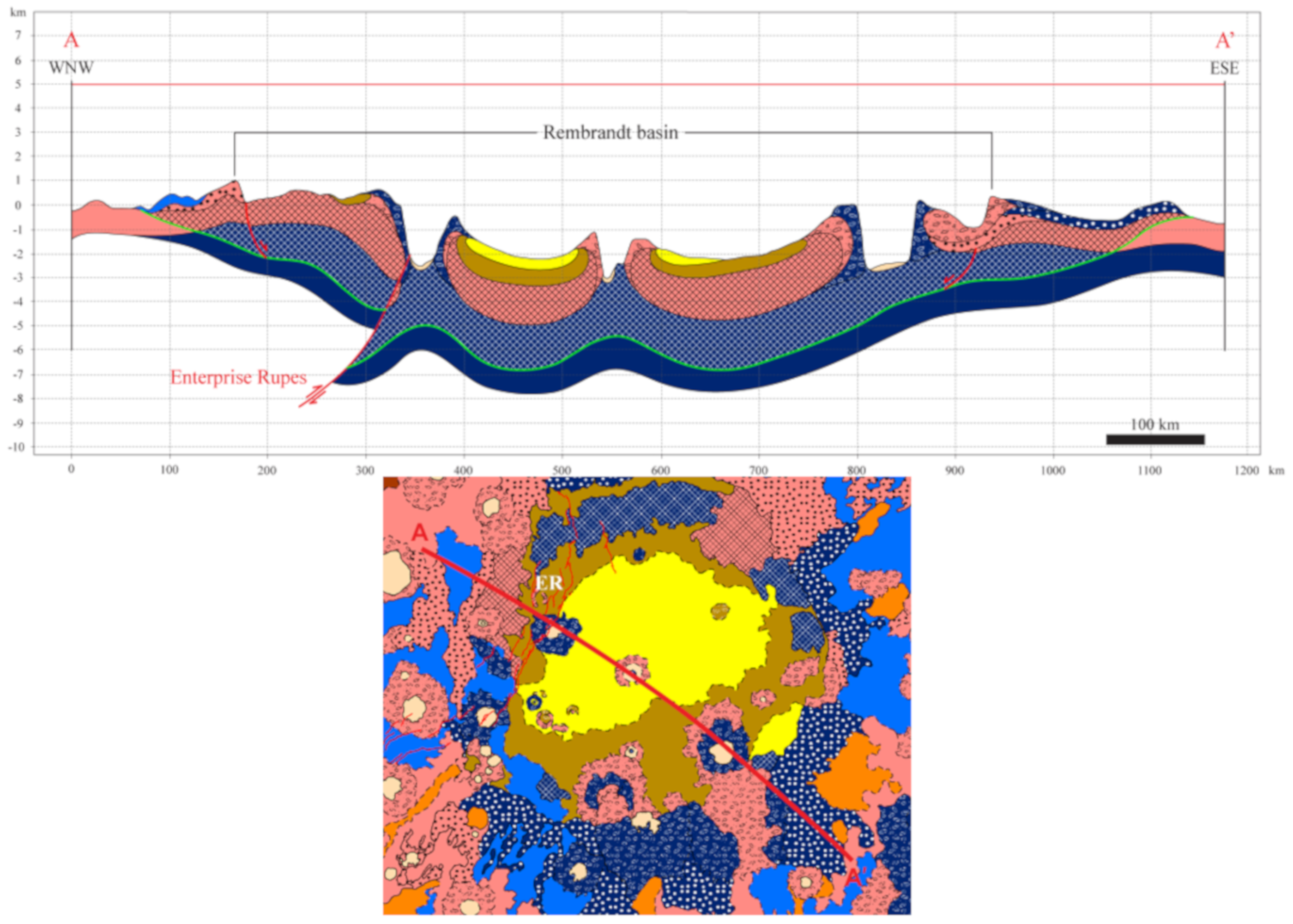
3.1.7. Main Tectonic Features

Within our maps we identified all tectonic structures. In particular, we mapped as “thrust” both lobate scarps and high-relief ridges, which are respectively asymmetrical landforms associated with thrust faults [48,55,56,57,58] and symmetrical narrow ridges associated with buried high-angle reverse faults [56,57,58,59,60]. More limited in length and with lower amount of displacement are wrinkle ridges [61,62,63], i.e., other landforms associated with thrust faults but commonly observed within volcanic plains [57,58,64]. Furthermore, in the W-NW portion the Rembrandt basin is crosscut by an extensive lobate scarp, i.e., the Enterprise Rupes, which we identified within both maps with the label “ER”. All these tectonic structures are interpreted as evidence of planetary cooling and contraction [27,48,56,64,65,66].

In addition, the smooth plains inside the Rembrandt basin are modified by multiple sets of contractional and extensional tectonic structures, developed both radially and concentrically towards the center of the basin [24,25]. Other major impact craters on Mercury, such as the Caloris basin, display similar pattern and structures [45,67,68]. Therefore, we chose to distinguish two main features: contractional (e.g., thrust faults and wrinkle ridges) and extensional (e.g., grabens).

In the SW portion of the map, another fault scarp extends up to the basin rim, known as Belgica Rupes (identified with the label “BR” within both maps). Along with Enterprise Rupes, this scarp system bounds a flat-floored, low-lying area that lies between the two scarps, with a mean width of ~400 km. Thrust motion on the two rupes has opposite sense of vergence. For further details regarding the kinematics of both fault systems and their crosscutting relations with the Rembrandt basin, the reader is referred to [44,69].

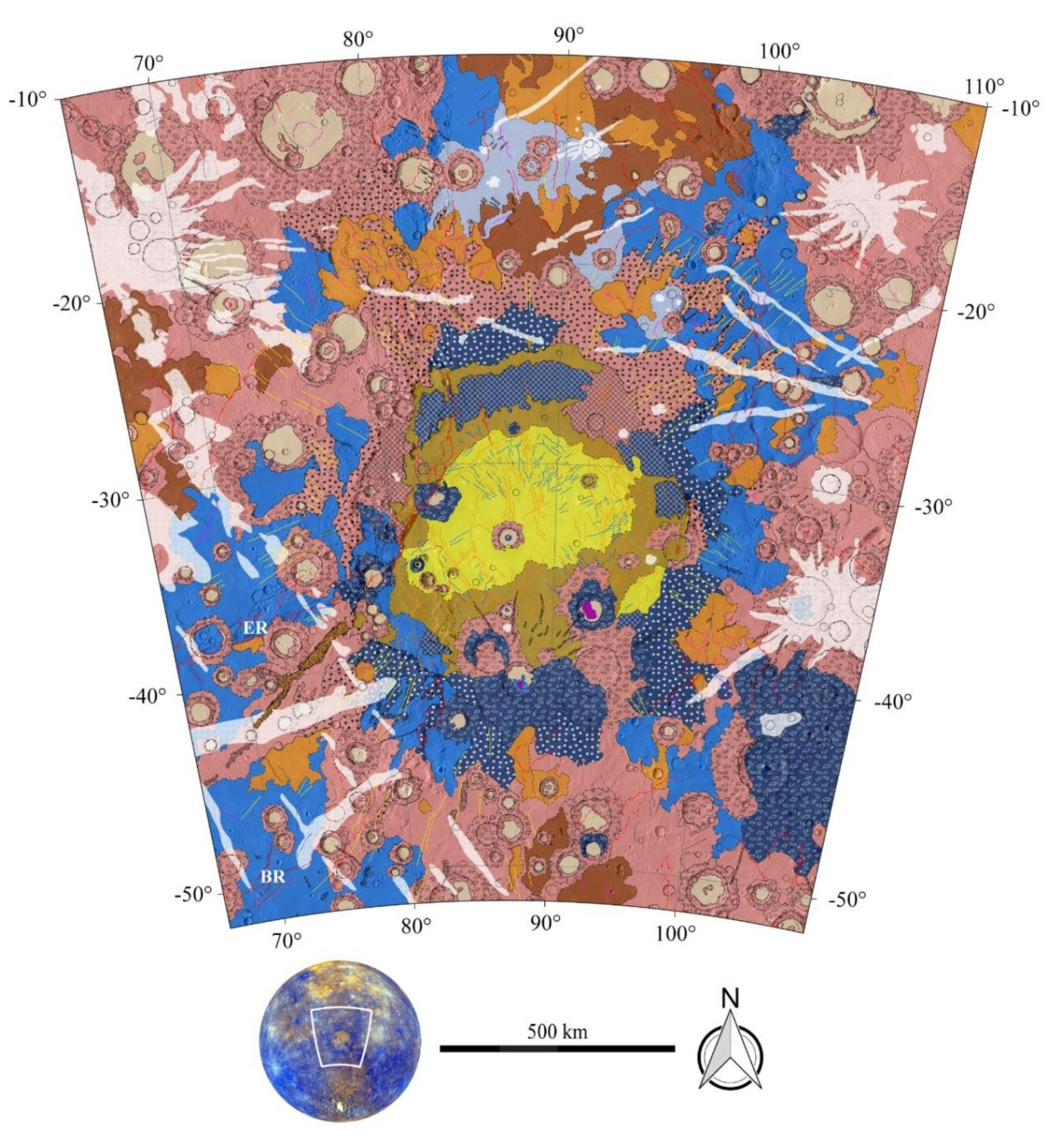
3.2. Geo-Stratigraphic Map Units

In this section we present the geo-stratigraphic map and its related units (Figure 4). A detail of the map units is presented in Figure 5.

3.2.1. Interior Smooth Plains

Considering the stratigraphic evolution of the Rembrandt basin, it is possible to infer that the basin floor is covered by a series of volcanism-related smooth plains (along with a potential base level of impact melt), rather than one single even (e.g., [25,26]).

Mapped as a single unit in the morpho-stratigraphic map (due to their similar crater density and surface morphology), these interior plains, indeed, show a subtle variation in tone in the color images [25], more noticeable in the Enhanced-Color mosaic (see Figure 1). This color variation is possibly associated with different volcanic flooding events. Therefore, we distinguished two different smooth plains units inside the basin, related to two distinct events corresponding to different relative and absolute model ages (discussed in Section 4.3). In particular, the unit mapped in the central portion, i.e., Younger interior smooth plains (YIP), has brighter color and higher albedo compared to the surrounding, i.e., Older interior smooth plains (OIP), suggesting less degradation of surface material by space weathering and therefore a younger age or a different composition [70,71].

3.2.2. Exterior Smooth Plains

Although they are distinguished into just two geologic units by morphological observations, the smooth plains outside the basin can be subdivided into four units taking into account their color variations (see the detail in Figure 5).

• High-reflectance exterior smooth plains (PrH). These plains appear distinctly as the brightest examples, with a similar tone to the youngest smooth plains inside the Rembrandt basin. PrH are also the smoothest and least cratered terrain found in the mapping area. As such, they can be considered the youngest event outside the basin. These plains are most likely to be related to a volcanic origin [26] (for the morphological characteristics, see ESP in the morpho-stratigraphic map).
• Low-reflectance exterior smooth plains (PrL). These plains are characterized by the darkest tone (in some places even similar to the low-reflectance material—see below) and are more heavily cratered than other smooth plains. These plains were attributed to impact melt by [26] (for the morphological characteristics, see EIP in the morpho-stratigraphic map). In the south-west portion of the basin, this material extends within the basin rim, suggesting that some impact melt might have been emplaced inside the basin, as well.
• Intermediate-reflectance Exterior Plains (PrI). We distinguished two additional plain units with different colors and albedo with respect to PrH and PrL. These plains, diverse in color and brightness one to each other, show an intermediate crater density with respect to the two end members. Therefore, from crater density and overlapping relationship, we can recognize the following stratigraphic sequence, from younger and brighter to older and darker units: PrH, PrI1, PrI2, PrL.

3.2.3. Intercrater Plains (IT)

These plains are related to the same unit described in the morpho-stratigraphy map layer as IT (see Section 3.1 for details). On the color images, these plains are hardly distinguishable from the surrounding material: they are found with a dark color (similar to the PrI2 and PrL) but distinctly brighter than the Low-reflectance material. The identification of these plains is mainly made by morphological characteristics (higher crater density and rougher surface texture).

The IT are found as both autochthonous or para-autochthonous material (the latter being uplifted by basin impact), respectively identified with the mapping codes IT and IT-pa). We also mapped IT as reworked material, excavated and ejected by either the Rembrandt basin itself (IT-r) or by subsequent impact craters (IT-r2). Within this map, we distinguished these materials as different units, maintaining the same fill color but with distinct pattern.

3.2.4. Low-Reflectance Material (LRM)

This material is thought to be the oldest material found on Mercury’s surface [72], and it is also used as stratigraphic marker due to its unique spectral properties [12]. Within the mapping area, this material is found as the darkest areas on the surface (within all color mosaics), with a dark blue color, and thus easily distinguished from the surrounding material (although in some cases, when excavated from small impact craters and covering PrL or IT, it displays a lighter color). LRM in this area is found as mainly allochthonous material, excavated from deep below the surface by the Rembrandt basin impact event, and subsequently reworked by other impact craters. Therefore, its color signature can be found in some parts of the basin’s proximal ejecta, and also inside the basin, where the smooth plains did not cover the basin floor, such as in the RFT. In fact, the RFT likely consists of para-autochthonous material, associated with either IT or LRM (respectively IT-pa and LRM-pa), which has been uplifted but not detached from the related pre-impact geologic units.

Furthermore, because the impact event was a very complex process, able to excavate and rework material coming from different sources and at different depths, it is hard to distinguish excavated LRM from other examples, since it is mostly found as regolith/breccias and reworked material covering the surface. Nonetheless, as for the IT, we were able to distinguish the LRM excavated from the Rembrandt basin (identified with the mapping code LRM-r) from that reworked by subsequent impact craters (LRM-r2). As for the IT, the distinction is highlighted by proper pattern.

In addition, it is likely that ejected material fell even within the basin, partially covering para-autochthonous material at its margins. However, as stated above, due to the complexity of the impact processes and lack of high-resolution surface information, we mapped ejected material (IT-r and LRM-r) only outside the basin.

We have not found direct evidence of autochthonous LRM on the surface of our study area, since this unit most likely lies below the basin floor.

3.2.5. Crater Material

As stated in Section 2.3, in the geo-stratigraphic map we mapped crater materials with the same color as the pristine geo-stratigraphic unit from which they are derived. However, a distinct overlying pattern indicates the allochthonous and reworked nature of these materials. Specifically, we distinguished crater material excavated and reworked by the Rembrandt basin itself (IT-r and LRM-r), from that excavated by subsequent impact craters (including IT-r2, LRM-r2, and also OIP-r2 within the basin).

Furthermore, many impact craters are filled with material that is smoother and brighter than their surroundings. We interpreted such material as either volcanic infill or impact melt, and hence not specifically attributable to any excavated stratigraphic unit. Therefore, we mapped these floors as a separate unit, as spectrally distinct (Volcanic) Crater Floor (VCF). Nonetheless, in some cases this infill shows the same color as the youngest exterior smooth plains, most probably indicating the same material composition. This consideration could lead to the geologic interpretation by which the smooth plains outside impact craters and confined within them were emplaced during the same event. Nonetheless, we chose to map them separately, since the volcanic plains infilling impact craters can be attributed to independent centers of effusion, and thus not always directly relatable to the surrounding smooth plains. Craters containing spectrally distinct floor material are widespread over the surface and can be as small as 5 km in diameter, but for the purpose of this work, which is to highlight the main geo-stratigraphic units, we mapped this unit only within craters with diameter > 20 km, being also consistent with craters mapped in the morpho-stratigraphic map. Some additional smaller craters within the Rembrandt basin were also identified to highlight spectrally distinct ejected material inside the basin.

In Figure 6 we present a close-up displaying a comparison between the two map layers produced in this work.

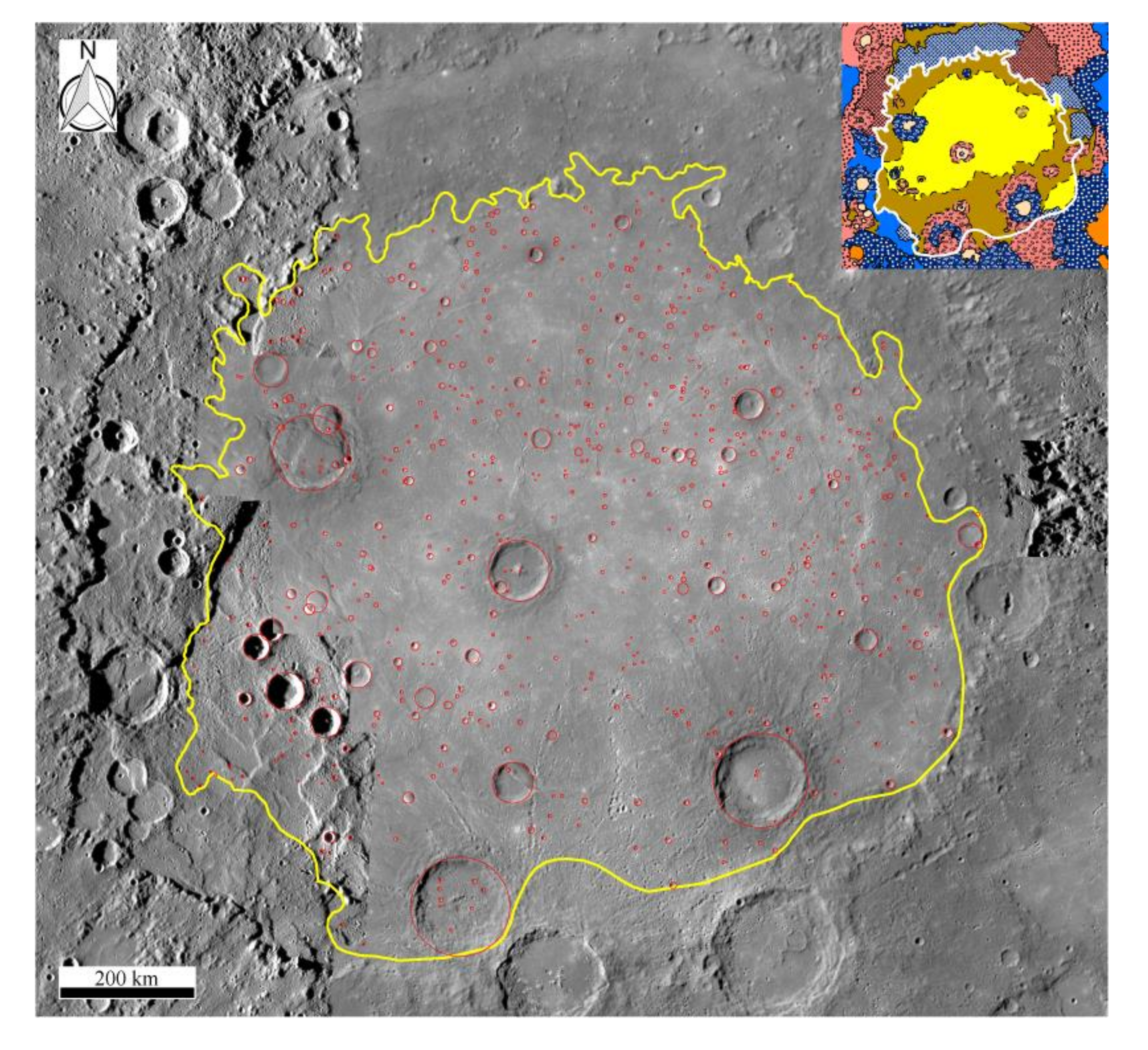
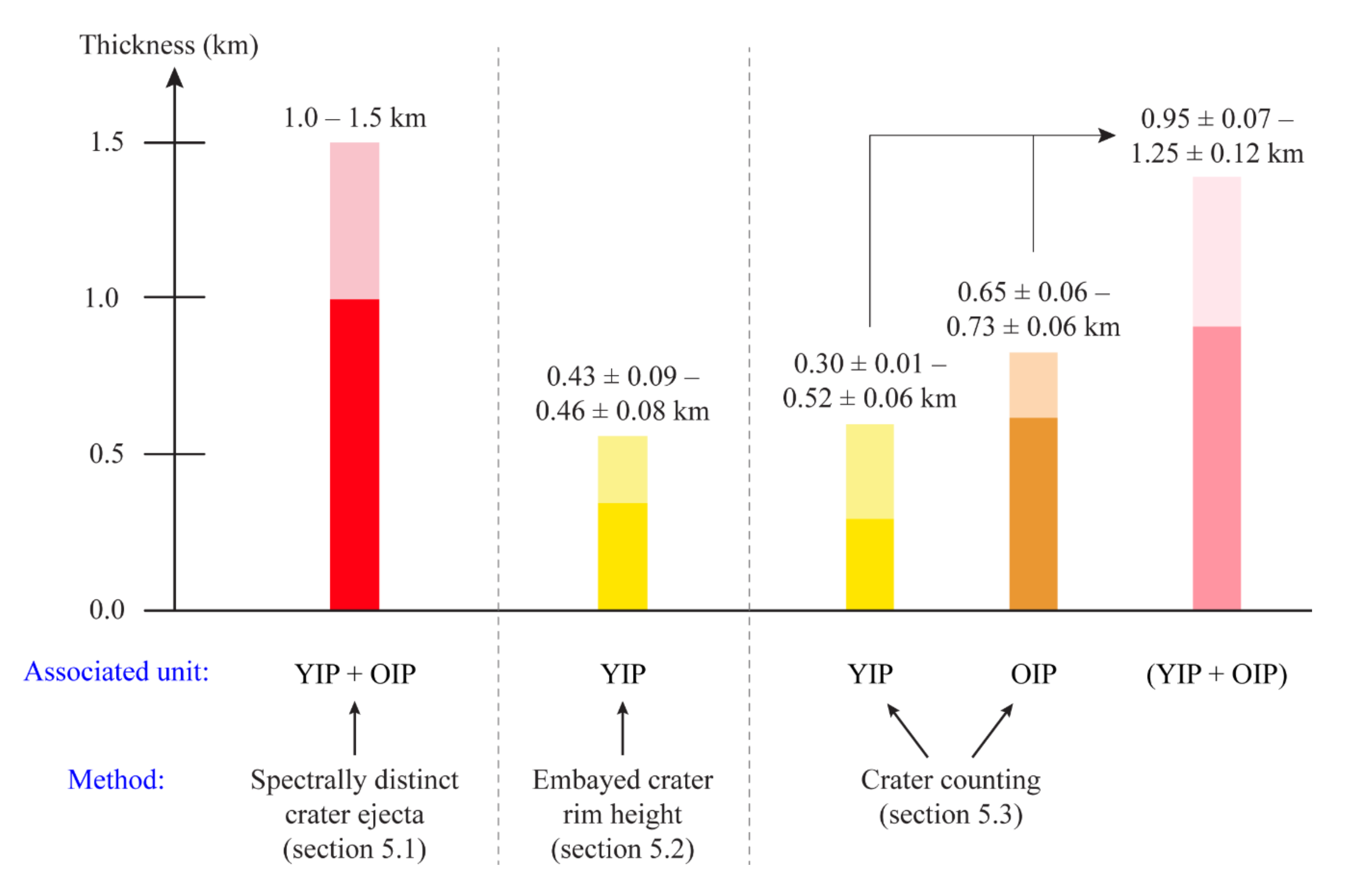
4. Thickness Estimated and Infilling History of the Rembrandt Basin

The geo-stratigraphic map reports two different infillings (YIP and OIP) and two base layers (LRM and IT) within the Rembrandt basin. This allowed us to proceed with thickness estimates of the two plain units, by applying several methods previously adopted by different authors [12,25,26] and merging them in a unified framework. In the following sections we present each method along with results and discussions. Subsequently, a final interpretation is given, together with our estimate of the total volume of lava infilling.

4.1. Spectrally Distinct Ejecta as Indicators of Maximum Thickness of Smooth Plains

An impact crater can provide a good insight into the local stratigraphy, in many different ways. [12] suggested that impact craters can be used as “well points” on the surface of Mercury, able to provide information on the depth and thickness of different geologic units. The maximum excavation depth of an impact crater (and therefore the maximum depth at which crater material is coming from) can be approximated to one-tenth the diameter of the related transient crater D_tc [73,74]. It is called “maximum” excavation depth, since it can be shallower for non-vertical impacts. Therefore, by attributing the ejecta deposits of each impact crater to the excavated geo-stratigraphic units, it is possible to derive their thicknesses.

If an impact exposes the same material composition as the surrounding unit (i.e., same color), which means that it does not penetrate other spectrally distinct units, the maximum excavation depth for that crater is an indicator of the minimum thickness for the surface layer. On the other hand, if an impact crater exposes spectrally distinct material (i.e., a different unit), the upper layer must be thinner than the value of the maximum excavation depth derived for that impact crater.

Consequently, following [12], we first measured rim-to-rim crater diameters D_r, and then derived the relative transient crater diameters D_tc using the scaling relationships found by [75], which are based on the following equation:

$$D_{tc}\approx C{D}_r^k$$

(1)

where following [75]:

$$k = 0.921$$

(2)

$$C = 0.758 D^{* 0.079}$$

(3)

We set the transition diameter D* between simple and complex craters on Mercury to 11.7 ± 1.2 km as determined by [76], in agreement with the values obtained by [77,78], who estimated D* respectively after NASA Mariner 10 and MESSENGER missions.

Following the method of [12], we analyzed spectrally distinct crater material in order to provide depth information for the geologic units where they occur. We furthermore derived the maximum excavation depth of impact craters within the YIP and OIP (Figure 7). In this case, we were interested in estimating the maximum thickness of the smooth plains inside the basin, identified as “bright material” in

Table 2. Analyzed Craters for which the maximum excavation depth was derived, along with the related thickness estimates.

Crater	Dr Measured	Maximum Excavation Depth 1	Excavated Unit 2	Minimum Thickness of Smooth Plains	Minimum Depth of Dark Material 3
1	44	3.00	DM		<3.0
2	11	0.84	BM	>0.84
3	13.5	1.01	BM	>1.01
4	13.5	1.01	BM	>1.01
5	21	1.52	BM	>1.52
6	13.5	1.01	BM	>1.01
7	10	0.77	BM	>0.77
8	21	1.52	DM		<1.52
9	31	2.18	DM		<2.18
10	6.5	0.52	BM	>0.52
11	10	0.77	DM		<0.77
12	11	0.84	BM	>0.84
13	59	3.94	DM		<3.94
14	24.5	1.75	DM		<1.75
15	39	2.05	DM		<2.05
16	17	1.25	BM	>1.25
17	19	1.39	DM		<1.39
18	9	0.70	BM	>0.70
19	9	0.70	BM	>0.70
20	8.5	0.66	BM	>0.66
21	23	1.65	DM		<1.65
22	73	4.79	DM		<4.79
23	79	5.15	DM		<5.15
24	67	4.42	DM		<4.42
25	16	1.18	DM		<1.18

¹ Values obtained from the equations derived by [75]. ² All values are expressed in km. “DM” stands for “Dark Material” (LRM, IT or potential “dark” impact melt), “BM” stands for “Bright Material” (YIP or OIP). See text for details. ³ Smooth plains are shallower than this value.

, as opposed to “dark material”, which includes spectrally distinct material related to either IT or LRM component (or even potential “dark” impact melt emplaced within to the basin—see PrL in Section 3.2).

Analysis of spectrally distinct crater ejecta constrains the thickness of the smooth plains inside the basin, and therefore the depth of the boundary between the smooth plains and the basin floor. Analyzing our results (Table 2), many impact craters within the basin were found excavating only bright material from a depth greater than 1 km (craters 3, 4, 5, 6 and 16), in some cases also 1.2 km close to the basin rim (Crater 16) and even 1.5 km in the center of the basin (crater 5). Other impact craters excavate dark material from a depth of 1.5–1.7 km (craters 8, 14 and 21), and in some cases at a depth of 1.2–1.4 km (craters 17 and 25), indicating that the smooth plains are thinner than these values. Moreover, Crater 11 excavates dark material from a depth of 0.8 km, suggesting thinning of the smooth plains in the northern part of the basin, close to the basin rim. However, considering all values, we are confident in deducing the average thickness of the smooth plains inside the Rembrandt basin (including both the YIP and OIP) to be in the range 1.0–1.5 km.

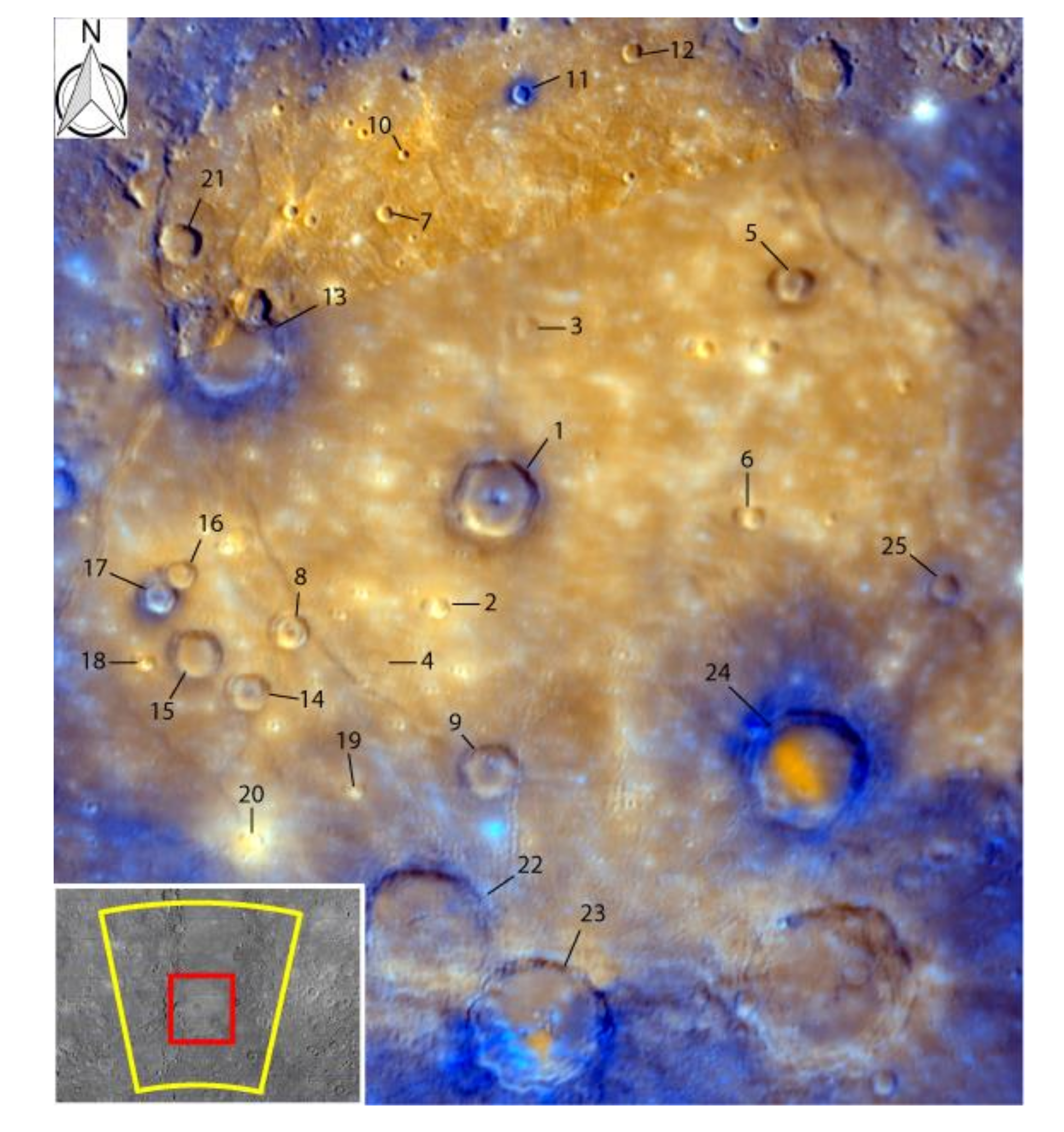
4.2. Measured vs. Predicted Rim Height of Embayed Craters as Thickness Estimates of Shallow Layers

Craters are “embayed” if a younger resurfacing event covers almost entirely its ejecta deposit, leaving only its rim exposed and visible (Figure 8), or “ghost”, when the crater is completely buried and filled up with lavas, including its rim, so that only the smoothed shape of the latter remains visible on the surface. When considering embayed craters, following the method used by [26] it is possible to estimate the overlapping plain thickness, by deriving the predicted rim height of that impact crater (before the resurfacing event), and then subtracting the measured rim height of the buried crater. Observing Figure 8, we determined the “measured rim height” by taking multiple profiles across each analyzed embayed or ghost crater and obtaining an average rim height. The “predicted rim height” was calculated using the following morphological relations for Mercurian craters, quantified by [76], who corrected previous equations obtained by [77,78] (respectively after Mariner 10 and MESSENGER flyby results):

$$h= \left(0.02\pm 0.01\right)D^{\left(1.19\pm 0.32\right)}$$

(4)

$$h=\left(0.25\pm 0.06\right)D^{\left(0.28\pm 0.06\right)}$$

(5)

where D is the measured rim-to-rim crater diameter and h is the predicted rim height before the emplacement of the plain lavas, distinguished in simple (4) and complex craters (5).

The estimated plain thickness is obtained as a difference between the predicted rim height and the measured rim height.

To avoid tectonic modification, which might lead to topographic variations comparable to or even exceeding the crater-rim elevations, we analyzed only embayed and ghost craters on flat plains close to the center of the basin, where post-emplacement tectonic processes are absent or negligible.

We found 3 embayed craters within the central portion of the basin (Figure 9) that were large enough to allow reliable thickness estimates. The results (

Table 3. Results from the analyzed embayed and ghost craters. All values are expressed in km. Errors are expressed in standard deviation.

Crater	Average Diameter	Measured Rim Height	σ Measured Rim Height	Predicted Rim Height	σ Predicted Rim Height	Plains Thickness	σ Plains Thickness
1 a	43.4	0.705	0.081	0.718	0.06	0.01 (≈ 0.00)	0.14
2 b	11.3	0.063	0.028	0.360	0.01 *	0.30 *	0.04
				0.493	0.06 **	0.43 **	0.09
3	13.5	0.075	0.028	0.518	0.06	0.44	0.09
4	13.7	0.058	0.017	0.520	0.06	0.46	0.08

^a Crater 1 (Bellini), being neither embayed or ghost crater, is used as a constraint to verify the reliability of the method, and returned a null value for the plain thickness (i.e., within the measurement error). ^b Crater 2 has a diameter that falls within the transition diameter between simple and complex crater, and therefore we present the results using both Equation (4) (values marked with *) and Equation (5) (values marked with **), respectively for simple and complex craters (see text for details). However, since this crater has a similar diameter to Crater 3 and 4, we kept the value obtained from the equation used for complex craters.

) suggest an average thickness of a surface layer of ~0.5 km (0.43 ± 0.09–0.46 ± 0.08 km including errors). We also analyzed a crater that is likely to be younger than the smooth plains (Bellini crater—Crater 1 in Table 3) due to its morphological characteristics (sharp rim and well-preserved ejecta deposits) and morphometry. For Bellini, the predicted rim height is equal (i.e., within the measurement error) to the measured rim height. In other words, the estimated thickness of the shallow layer resulted in a null value, indicating that this crater has not been covered by subsequent flows. Consequently, this crater provides an effective constraint on the reliability of the adopted method.

The value of ~0.5 km clearly differs from the values obtained with the previous method (see Section 4.1), which constrains the average thickness of the smooth plains (both YIP and OIP) to 1.0–1.5 km. As such, it is likely that the value of ~0.5 km represents the average thickness of the shallowest layer, associated with the youngest event, i.e., the YIP, and that craters 2, 3 and 4 formed on lower plains, presumably on the OIP, before the emplacement of YIP. Therefore, the underlying OIP likely reach an average thickness between 0.5–1 km.

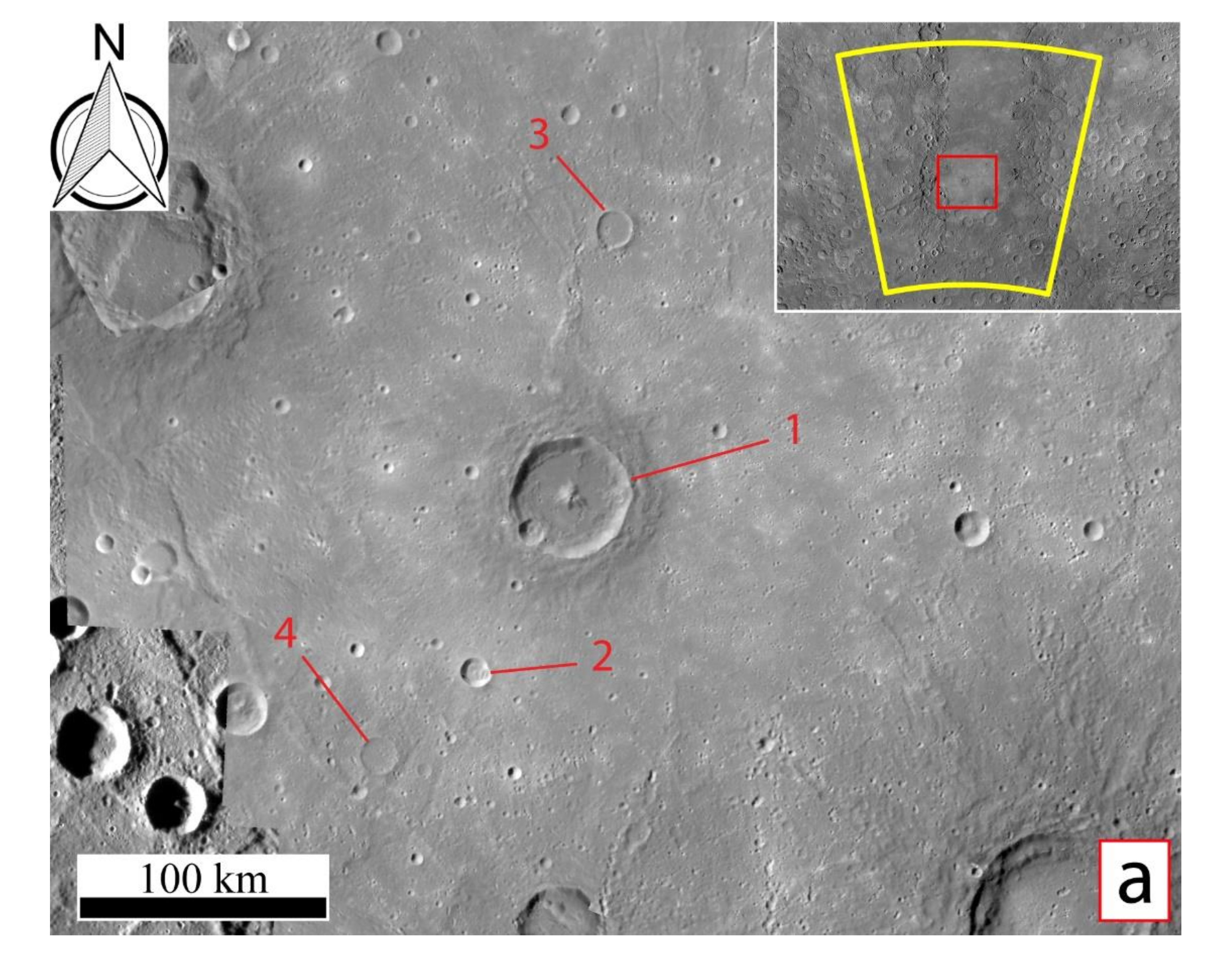
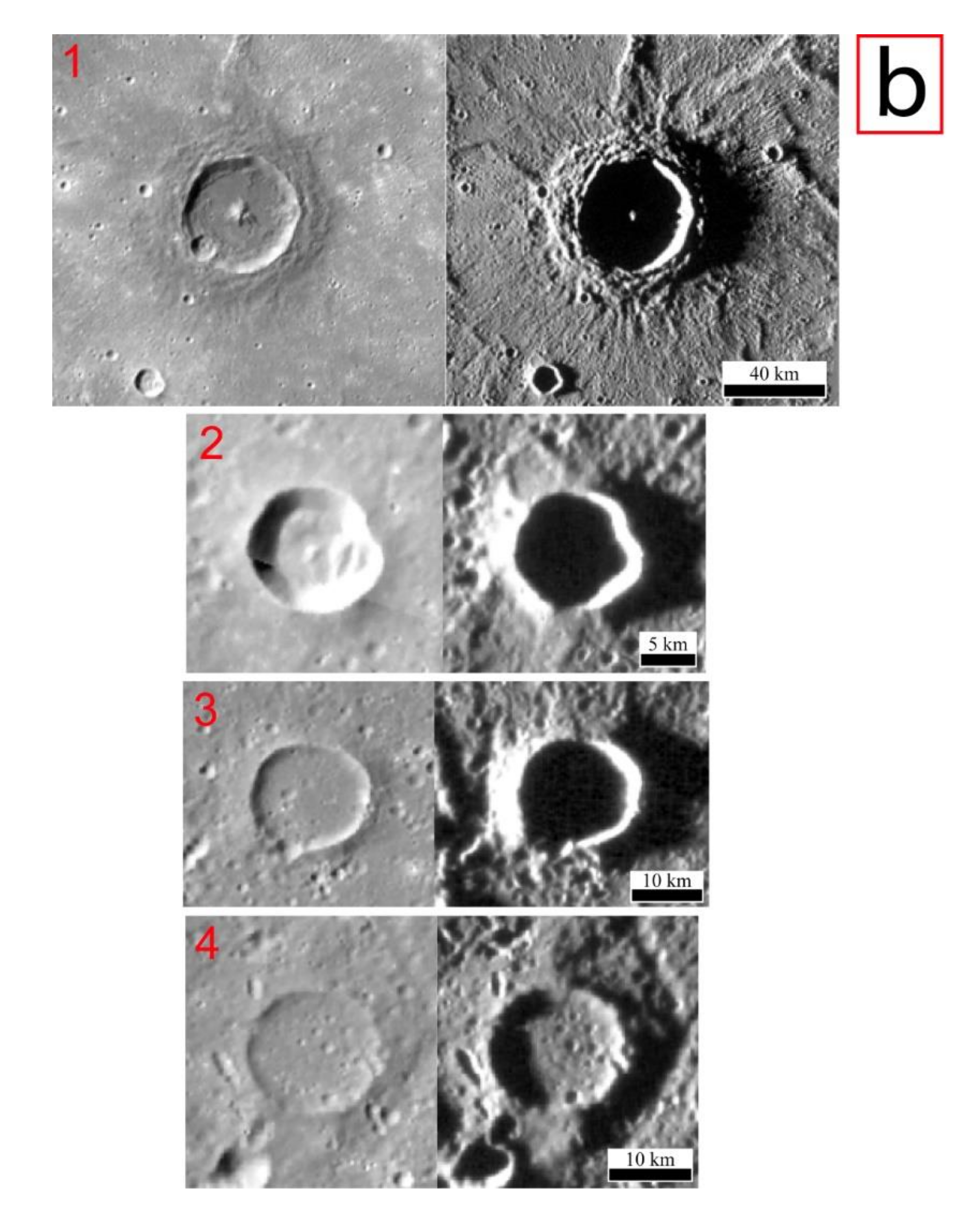
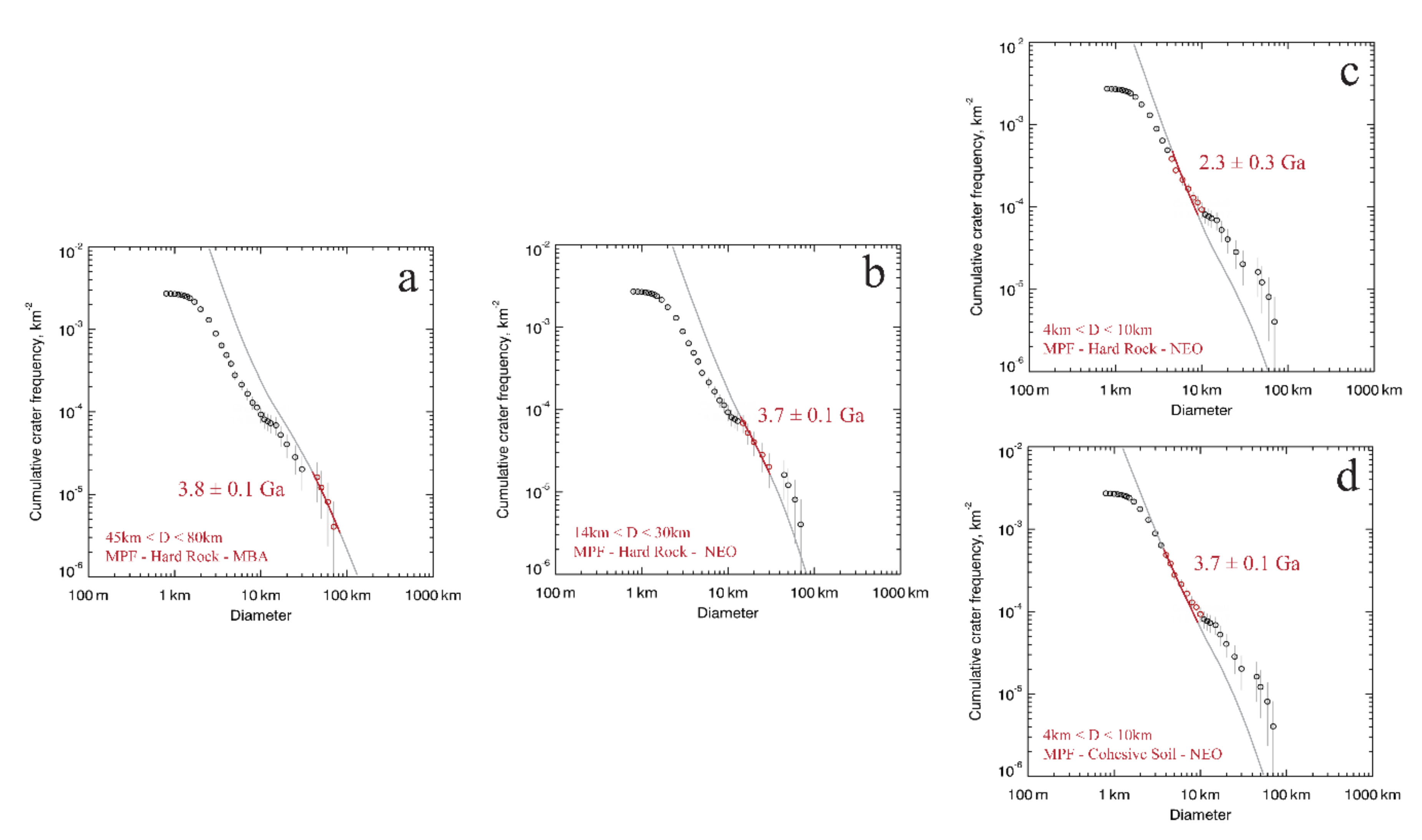
4.3. Crater Counting for Dating and Surface Layering Thickness Estimates

Several methods of age determination based on crater counting have been applied on many planetary surfaces and on different targets, aiming to obtain a model age of various surfaces [79,80,81,82]. Absolute model ages are assessed by relating the number and size of craters counted in a given area with the accumulation rate of craters (i.e., impactor flux) in a target body. Such flux is derived from dynamic models of the Main Belt Asteroids (MBAs) and Near-Earth Objects (NEOs), and converted into Crater Size-Frequency Distributions (CSFDs) through calibration with radiometric ages of different regions on the Moon’s surface [83]. In addition, cumulative crater counting can be used to infer surface layering, due to resurfacing processes (e.g., volcanic flows [25,84]).

Considering the stratigraphic evolution of the Rembrandt basin, many of the subdued craters that are observed within the smooth plains were not actually formed on the shallowest (i.e., the youngest) surface layer, but on deeper older layers. This is the case of ghost and embayed craters described in the previous section. As a result, if included within CSFDs, these craters can produce an S-shaped kink, with an apparent lower frequency of smaller craters, since those formed on an older surface were efficiently hidden by later resurfacing events. This kink, therefore, can be related to a surface layering.

Furthermore, following [25], by extracting from the CSFD the minimum and maximum diameter values at which these kinks occur, it is possible to convert these values into minimum and maximum thickness of the plain layers that must have covered those craters. This conversion is made by applying the same exponential laws derived by [76] and described in the previous section.

In this case, the result consists of an average thickness of the shallower unit responsible for the resurfacing events, whereas on the previous methods the results were derived as point information, referred to the analyzed impact craters.

Hence, to identify possible multiple events and surface layering, all impact craters were taken into account when producing the CSFD plot, including ghost and embayed craters. However, we avoided chains and clusters of craters that may be associated with secondary impacts (Figure 10).

We performed crater counting and obtained the cumulative crater-count distribution using the CraterTools add-on for ArcMap [85], and subsequently analyzed the cumulative plot with the Craterstats2 software [86]. We applied the Model Production Function of [81] using both the Hard Rock and the Cohesive Soil scaling laws to fit the different portions of the CSFD. In particular, the Cohesive Soil regime is applied to smaller craters that affect only the upper cohesionless regolith and fractured layers, while larger craters affecting the unfractured bedrock form on the Hard-Rock regime. The transition from one regime to the other occurs at different depth (and therefore crater size), depending on the planetary body and the target area [81,83].

Therefore, we applied the Model Production Function on the smooth plains inside the Rembrandt basin, in order to derive model ages and potential surface layering (i.e., observing the kinks from which the thickness of resurfacing events is derived). Results are displayed in Figure 11.

Results from the Model Production Function best fits display different model ages that can be associated with different geologic events related to the impact basin:

• The age of 3.8 ± 0.1 Ga (Figure 11a) is likely to be associated with RFT, mapped and interpreted as the bottom layer within the basin, i.e., a mixture of LRM and IT reworked in the early stages after the impact event and before the emplacement of the smooth plains. Therefore, this age can be related to the Rembrandt basin impact event, being also consistent with previous works [24,25].
• Secondly, we link the age of 3.7 ± 0.1 Ga (Figure 11b) to the emplacement of the first smooth plain event, i.e., the OIP: although this value falls within the fit error of the previous age, the two different fits are separated by a visible S-shape kink that occurs between 30–45 km.
• Lastly, CSFD for craters with diameter <10 km resulted in ambiguous age assessments:

  a.

  The Hard-Rock scaling law (Figure 11c) suggests the presence of a resurfacing event, significantly distinct in terms of age from the OIP and indeed possibly associated with the YIP of 2.3 ± 0.3 Ga.

  b.

  Using the Cohesive Soil scaling law (Figure 11d), which is consistent with fractured material (i.e., breccias) expected for smaller crater sizes [81], the resulting CSFD at craters <10 km returns an age of 3.7 ± 0.1 Ga. This suggests a continuity in the filling process of smooth plains within the basin, being the same age of 3.7 ± 0.1 Ga for all craters with diameter <30 km. According to this interpretation, the YIP and OIP (well visible in the geo-stratigraphic map) are not separable in terms of model age, since they pertain to two phases of the same infilling event developed in the time bracket of the model-age error bar (i.e., 100 Ma).

Considering the CSFD for craters <10 km, following the first explanation, the kink reflects the resurfacing event that covered most of the smaller old craters. According to the second explanation, the S-shaped kink occurring between 10–14 km should be attributed to the Hard Rock–Cohesive Soil change in scaling law (e.g., [83,84]).

Assuming that all the kinks (at 10–14 km and 30–45 km) are due to the emplacement of younger layers of smooth plains associated with volcanic resurfacing, we were able to use the relationships derived by [76] described in Section 4.2 to convert these diameter ranges into minimum and maximum thickness of multiple surface layers. By doing so, the results are thickness values ranging between 0.30 ± 0.01 km and 0.52 ± 0.06 km for the upper layer (the kink at 10–14 km), and between 0.65 ± 0.06 km and 0.73 ± 0.06 km for the lower layer (the kink at 30–45 km).

These values are highly consistent with the thickness values obtained with previous methods. In particular, the value of 0.30 ± 0.01–0.52 ± 0.06 km is consistent with the thickness of ~0.5 km of the YIP obtained analyzing embayed craters (see Section 4.2). Furthermore, the value of 0.65 ± 0.06–0.73 ± 0.06 km (approximated to ~0.7 km) can be associated with an older resurfacing event, hence likely referred to the OIP. In fact, taken together, these average thickness values obtained for the YIP and OIP are consistent with the total thickness of the volcanic infilling of the Rembrandt basin, estimated between 1.0–1.5 km by analyzing spectrally distinct crater ejecta (see Section 4.1).

Hence, given the consistency among the different methods of thickness estimates, which confirm the presence of an additional resurfacing event, we believe that the cratering model age obtained using the Hard-Rock scaling law is indeed the most reliable also for the small crater sizes (Figure 11c), and constrains the last volcanic emplacement event within the Rembrandt basin at 2.3 Ga.

In Figure 12, we present a summary of all values obtained from thickness estimates, for an overall comprehension of the results and a better understanding of the smooth plain layering inside the Rembrandt basin.

4.4. Volume Estimate of the Basin Infilling

We provided volume estimates for the smooth plains inside the Rembrandt basin, assuming these units as cylindrical bodies and considering the area of the related mapped polygons, along with the maximum thickness values we obtained in this work (thus the volume estimate represents a maximum value). With an area of ~2.5 × 10⁵ km² (including the YIP and the OIP) and an average thickness between 1.0–1.5 km, the estimated volume becomes 2.5–3.7 × 10⁵ km³. These may be compared with those obtained by [22] for the Caloris basin, where the interior smooth plains were estimated of 3.2–5.2 × 10⁶ km³, being also thicker than those of the Rembrandt basin (1.5–3.5 km—see [22]). This seems to be reasonable given the smaller size of Rembrandt basin with respect to Caloris and the likely lesser excavation depth.

5. Discussions

Given that the morpho-stratigraphic map and the integrated geo-stratigraphic map both try to relate the different units in a sequence of geologic events, it is possible to infer a stratigraphic correlation between the units inside and outside the basin in each map. The relations among the different units, also comparing the two maps, are shown on the stratigraphic columns in Figure 13. In addition, the geologic section of Figure 14 shows the thicknesses of the different layers of the geo-stratigraphic map, the connection between the ejecta of the larger craters and their deep sources, and the relationships between the allochthonous, autochthonous, and para-autochthonous materials.

The main similarities and differences among the two maps and the related implications for the geologic evolution of the Rembrandt basin and its units are summarized in the following points:

• The Intercrater plains (IT) and the Low-Reflectance Material (LRM) of the geo-stratigraphic map, attributed to the pre-Tolstojan and Tolstojan age [19], correspond in the morpho-stratigraphic map to the Intercrater plains (IT) as well as the ejecta (RE) and rough floor (RFT) of the Rembrandt basin. It is worth recalling here that while the pristine IT are thought to pre-date the Rembrandt basin impact, the LRM has been interpreted as uplifted basin floor material from lower crust or upper mantle [22,26] or crystallized (and differentiated?) impact melt [88], so it can be either related to the impact or pre-date it. However, in our geo-stratigraphic map and chart we have specifically distinguished the following materials:

  a.

  Autochthonous pre-impact material (IT and LRM)

  b.

  Syn-impact para-autochthonous material (uplifted but not detached) (IT-pa and LRM-pa—which are associated with the RFT in the morpho-stratigraphic map)

  c.

  Post-impact material, reworked by the Rembrandt impact itself (IT-r and LRM-r)

  d.

  Material reworked by subsequent impact craters (IT-r2 and LRM-r2)

The relationships among these units are addressed in Figure 14.

2.

The smooth plains are broadly unified in three large units within and outside the basin in the morpho-stratigraphic map, whereas they are subdivided into several emplacement events in the geo-stratigraphic map. Within the geo-stratigraphic map, in particular, we distinguished two different smooth plain units inside the Rembrandt basin, associated with two different volcanic resurfacing events that occurred after the impact basin. Model-age results for the younger smooth plains (YIP) suggest either early-Calorian or mid-Calorian age (considering the age boundaries proposed by [87]), using respectively the Cohesive Soil or Hard-Rock production function for smaller craters. Analysis of the S-shaped kinks obtained by using the Hard-Rock production function returned thickness estimates consistent with those derived by independent methods (see Section 4) and thus the mid-Calorian age seems more reliable. This means that the volcanic activity within the Rembrandt basin would have been maintained much longer (up to 2.3 Ga instead of 3.5 Ga) than generally thought for most of the Mercury surface (e.g., [8]) being coeval to the younger volcanism up to date documented only in a few other minor basins [89].

3.

Our volume estimate of the entire Rembrandt infilling is around 2.5–3.7 × 10⁵ km³. This is appreciably lower than that of the larger Caloris basin, which was flooded by a volume ranging between 3.2 and 5.2 × 10⁶ km³ [22]. It is thus reasonable that the first lava infilling of the two basins was of similar early-Calorian age [4,21,25], but the volume of lava infilling much greater in Caloris than in Rembrandt.

4.

The crater deposits are considered in totally different ways in the morpho-stratigraphic and geo-stratigraphic maps. The former is more informative about their relative age, constrained by the degradation degree, whereas the latter attempts to distinguish the original source of their materials. How best to combine these two types of information is still to be evaluated in function of map readability and purpose.

It is, therefore, evident that the classification criteria of the units in the morpho-stratigraphic and geo-stratigraphic maps are different and not unifiable in a single map layer. In fact, the first one is devoted to morphological features and textures and the latter one enables more accurate stratigraphic classification and thus detailed reconstruction of the crustal geologic evolution. In terms of relative age discrimination, the morpho-stratigraphic approach is more effective for crater materials, whereas the geo-stratigraphic one can better discriminate the superposition among older units.

6. Conclusions

We produced two distinct geologic maps of Rembrandt basin, displaying complementary geologic information. The first map layer is focused on geomorphology and morpho-stratigraphy, following the methods adopted in the production of geologic maps of the Mercury quadrangles. The second map layer is based on main geo-stratigraphic units, which can be related to different events, and thus different ages; these can be distinguished by color variegation, reflecting their different material composition or relative exposure age. Crater floors, ejecta deposits, and central peak structures were classified depending on the color-stratigraphic unit they are constituted of, neglecting their degradation state. The geo-stratigraphic map is thus more effective for differentiating autochthonous and reworked material coming from the same source. Moreover, in this map, we were able to distinguish four different smooth plains units in the area surrounding the Rembrandt basin (PrH, PrI1, PrI2, PrL), and two units inside the basin itself (YIP and OIP). By contrast the morpho-stratigraphic map is more effective in discriminating the relative age of the crater materials, based on the degradation classes defined by morphological characteristics. Future attempts should be devoted in integrating the more informative fields of each map.

Analyzing spectrally distinct crater ejecta inside the basin, we estimated the total average thickness of the volcanic infilling inside the Rembrandt basin to be between 1.0 and 1.5 km. Furthermore, measuring the rim height of embayed and ghost craters, we bound the average thickness for the youngest volcanic event, the YIP, at ~0.5 km. S-shaped kinks in the crater size-frequency distribution confirm the same thickness value of the YIP and also suggest an average thickness of ~0.7 km for the older event, the OIP. Taken together, these values are consistent with the total thickness of the volcanic resurfacing, mentioned above.

Model ages suggest an age of 3.8 ± 0.1 Ga for the Rembrandt basin impact (which is consistent with [24,25]) and possibly two distinct volcanic resurfacing events, the oldest yielding an ending age of 3.7 ± 0.1 Ga and the youngest of 2.3 ± 0.3 Ga. The second event implies extensive lava emplacement on Mercury even in the mid-Calorian, up to an age of 2.3 Ga.

The integrated mapping of the Rembrandt basin area provides important references for the ongoing ESA-JAXA BepiColombo mission to Mercury, supporting target selection for the Spectrometer and Imaging for MPO (Mercury Planetary Orbiter) BepiColombo Integrated Observatory SYStem (SIMBIO-SYS) payload [90].

References

1. Hargitai, H. Planetary Cartography and GIS; Springer International Publishing: Berlin/Heidelberg, Germany, 2019. [Google Scholar]
2. Spudis, P.D.; Guest, J.E. Stratigraphy and geologic history of Mercury. In Mercury; University of Arizona Press: Tucson, AZ, USA, 1988; pp. 118–164. [Google Scholar]
3. Denevi, B.W.; Robinson, M.S.; Solomon, S.C.; Murchie, S.L.; Blewett, D.T.; Domingue, D.L.; McCoy, T.J.; Ernst, C.M.; Head, J.W.; Watters, T.R.; et al. The evolution of Mercury’s crust: A global perspective from MESSENGER. Science 2009, 324, 613–618. [Google Scholar] [CrossRef] [PubMed]
4. Denevi, B.W.; Ernst, C.M.; Meyer, H.M.; Robinson, M.S.; Murchie, S.L.; Whitten, J.L.; Head, J.W.; Watters, T.R.; Solomon, S.C.; Ostrach, L.R.; et al. The distribution and origin of smooth plains on Mercury. J. Geophys. Res. E Planets 2013, 118, 891–907. [Google Scholar] [CrossRef] [Green Version]
5. Rothery, D.A. Planet Mercury: From Pale Pink Dot to Dynamic World; Springer: Berlin/Heidelberg, Germany, 2014. [Google Scholar]
6. Ostrach, L.R.; Robinson, M.S.; Whitten, J.L.; Fassett, C.I.; Strom, R.G.; Head, J.W.; Solomon, S.C. Extent, age, and resurfacing history of the northern smooth plains on Mercury from MESSENGER observations. Icarus 2015, 250, 602–622. [Google Scholar] [CrossRef]
7. Prockter, L.M.; Head, J.W.I.I.I.; Byrne, P.K.; Denevi, B.W.; Kinczyk, M.J.; Fassett, C.I.; Whitten, J.L.; Thomas, R.J.; Ernst, C.M. The First Global Geological Map of Mercury. In Proceedings of the 47th Lunar and Planetary Science Conference, The Woodlands, TX, USA, 21–25 March 2016; Lunar and Planetary Institute: Houston, TX, USA, 2016; p. 1245. [Google Scholar]
8. Byrne, P.K.; Ostrach, L.R.; Fassett, C.I.; Chapman, C.R.; Denevi, B.W.; Evans, A.J.; Klimczak, C.; Banks, M.E.; Head, J.W.; Solomon, S.C. Widespread effusive volcanism on Mercury likely ended by about 3.5 Ga. Geophys. Res. Lett. 2016, 43, 7408–7416. [Google Scholar] [CrossRef] [Green Version]
9. Denevi, B.W.; Chabot, N.L.; Murchie, S.L.; Becker, K.J.; Blewett, D.T.; Domingue, D.L.; Ernst, C.M.; Hash, C.D.; Hawkins, S.E.; Keller, M.R.; et al. Calibration, Projection, and Final Image Products of MESSENGER’s Mercury Dual Imaging System. Space Sci. Rev. 2018, 214. [Google Scholar] [CrossRef]
10. Solomon, S.C.; Nittler, L.R.; Anderson, B.J. Mercury: The View after MESSENGER; Cambridge University Press: Cambridge, UK, 2018. [Google Scholar]
11. Melosh, H.J.; Dzurisin, D. Mercurian global tectonics: A consequence of tidal despinning? Icarus 1978, 35, 227–236. [Google Scholar] [CrossRef]
12. Ernst, C.M.; Murchie, S.L.; Barnouin, O.S.; Robinson, M.S.; Denevi, B.W.; Blewett, D.T.; Head, J.W.; Izenberg, N.R.; Solomon, S.C.; Roberts, J.H. Exposure of spectrally distinct material by impact craters on Mercury: Implications for global stratigraphy. Icarus 2010, 209, 210–223. [Google Scholar] [CrossRef]
13. Peplowski, P.N.; Lawrence, D.J.; Feldman, W.C.; Goldsten, J.O.; Bazell, D.; Evans, L.G.; Head, J.W.; Nittler, L.R.; Solomon, S.C.; Weider, S.Z. Geochemical terranes of Mercury’s northern hemisphere as revealed by MESSENGER neutron measurements. Icarus 2015, 253, 346–363. [Google Scholar] [CrossRef]
14. Weider, S.Z.; Nittler, L.R.; Starr, R.D.; Crapster-Pregont, E.J.; Peplowski, P.N.; Denevi, B.W.; Head, J.W.; Byrne, P.K.; Hauck, S.A.; Ebel, D.S.; et al. Evidence for geochemical terranes on Mercury: Global mapping of major elements with MESSENGER’s X-Ray Spectrometer. Earth Planet. Sci. Lett. 2015, 416, 109–120. [Google Scholar] [CrossRef]
15. Namur, O.; Charlier, B. Silicate mineralogy at the surface of Mercury. Nat. Geosci. 2017, 10, 9–13. [Google Scholar] [CrossRef]
16. Bott, N.; Doressoundiram, A.; Zambon, F.; Carli, C.; Guzzetta, L.; Perna, D.; Capaccioni, F. Global Spectral Properties and Lithology of Mercury: The Example of the Shakespeare (H-03) Quadrangle. J. Geophys. Res. Planets 2019, 124, 2326–2346. [Google Scholar] [CrossRef]
17. Mancinelli, P.; Minelli, F.; Pauselli, C.; Federico, C. Geology of the Raditladi quadrangle, Mercury (H04). J. Maps 2016, 12, 190–202. [Google Scholar] [CrossRef] [Green Version]
18. Galluzzi, V.; Guzzetta, L.; Ferranti, L.; Di Achille, G.; Rothery, D.A.; Palumbo, P. Geology of the Victoria quadrangle (H02), Mercury. J. Maps 2016, 12, 227–238. [Google Scholar] [CrossRef]
19. Guzzetta, L.; Galluzzi, V.; Ferranti, L.; Palumbo, P. Geology of the Shakespeare quadrangle (H03), Mercury. J. Maps 2017, 13, 227–238. [Google Scholar] [CrossRef] [Green Version]
20. Wright, J.; Rothery, D.A.; Balme, M.R.; Conway, S.J. Geology of the Hokusai quadrangle (H05), Mercury. J. Maps 2019, 15, 509–520. [Google Scholar] [CrossRef]
21. Strom, R.G.; Banks, M.E.; Chapman, C.R.; Fassett, C.I.; Forde, J.A.; Head, J.W.; Merline, W.J.; Prockter, L.M.; Solomon, S.C. Mercury crater statistics from MESSENGER flybys: Implications for stratigraphy and resurfacing history. Planet. Space Sci. 2011, 59, 1960–1967. [Google Scholar] [CrossRef]
22. Ernst, C.M.; Denevi, B.W.; Barnouin, O.S.; Klimczak, C.; Chabot, N.L.; Head, J.W.; Murchie, S.L.; Neumann, G.A.; Prockter, L.M.; Robinson, M.S.; et al. Stratigraphy of the Caloris basin, Mercury: Implications for volcanic history and basin impact melt. Icarus 2015, 250, 413–429. [Google Scholar] [CrossRef]
23. Murchie, S.L.; Klima, R.L.; Denevi, B.W.; Ernst, C.M.; Keller, M.R.; Domingue, D.L.; Blewett, D.T.; Chabot, N.L.; Hash, C.D.; Malaret, E.; et al. Orbital multispectral mapping of Mercury with the MESSENGER Mercury Dual Imaging System: Evidence for the origins of plains units and low-reflectance material. Icarus 2015, 254, 287–305. [Google Scholar] [CrossRef]
24. Watters, T.R.; Head, J.W.; Solomon, S.C.; Robinson, M.S.; Chapman, C.R.; Denevi, B.W.; Fassett, C.I.; Murchie, S.L.; Strom, R.G. Evolution of the Rembrandt impact basin on Mercury. Science 2009, 324, 618–621. [Google Scholar] [CrossRef]
25. Ferrari, S.; Massironi, M.; Marchi, S.; Byrne, P.K.; Klimczak, C.; Martellato, E.; Cremonese, G. Age relationships of the Rembrandt basin and Enterprise Rupes, Mercury. Geol. Soc. Spec. Publ. 2015, 401, 159–172. [Google Scholar] [CrossRef]
26. Whitten, J.L.; Head, J.W. Rembrandt impact basin: Distinguishing between volcanic and impact-produced plains on Mercury. Icarus 2015, 258, 350–365. [Google Scholar] [CrossRef]
27. Watters, T.R.; Solomon, S.C.; Robinson, M.S.; Head, J.W.; André, S.L.; Hauck, S.A.; Murchie, S.L. The tectonics of Mercury: The view after MESSENGER’s first flyby. Earth Planet. Sci. Lett. 2009, 285, 283–296. [Google Scholar] [CrossRef]
28. Klimczak, C.; Byrne, P.K.; Solomon, S.C. A rock-mechanical assessment of Mercury’s global tectonic fabric. Earth Planet. Sci. Lett. 2015, 416, 82–90. [Google Scholar] [CrossRef]
29. Massironi, M.; Di Achille, G.; Rothery, D.A.; Galluzzi, V.; Giacomini, L.; Ferrari, S.; Zusi, M.; Cremonese, G.; Palumbo, P. Lateral ramps and strike-slip kinematics on Mercury. Geol. Soc. Spec. Publ. 2015, 401, 269–290. [Google Scholar] [CrossRef]
30. Crane, K.T.; Klimczak, C. Tectonic patterns of shortening landforms in Mercury’s northern smooth plains. Icarus 2019, 317, 66–80. [Google Scholar] [CrossRef]
31. Giacomini, L.; Massironi, M.; Galluzzi, V.; Ferrari, S.; Palumbo, P. Dating long thrust systems on Mercury: New clues on the thermal evolution of the planet. Geosci. Front. 2020, 11, 855–870. [Google Scholar] [CrossRef]
32. Hawkins, S.E.; Boldt, J.D.; Darlington, E.H.; Espiritu, R.; Gold, R.E.; Gotwols, B.; Grey, M.P.; Hash, C.D.; Hayes, J.R.; Jaskulek, S.E.; et al. The Mercury dual imaging system on the MESSENGER spacecraft. Space Sci. Rev. 2007, 131, 247–338. [Google Scholar] [CrossRef]
33. Becker, K.J.; Robinson, M.S.; Becker, T.L.; Weller, L.A.; Edmundson, K.L.; Neumann, G.A.; Perry, M.E.; Solomon, S.C. First global digital elevation model of Mercury. In Proceedings of the 47th Lunar and Planetary Science Conference, The Woodlands, TX, USA, 21–25 March 2016; Lunar and Planetary Institute: Houston, TX, USA, 2016; p. 2959. [Google Scholar]
34. Deetz, C.H.; Adams, O.S. Elements of Map Projection with Applications to Map and Chart Construction, 5th ed.; US Coast and Geodetic Survey Special Publication 68; U.S. Department of Commerce: Washington, DC, USA, 1945. [Google Scholar]
35. Galluzzi, V. Multi-mapper projects: Collaborative Mercury mapping. In Planetary Cartography and GIS; Springer: Berlin/Heidelberg, Germany, 2019; pp. 207–218. [Google Scholar]
36. Shoemaker, E.; Hackman, R.J. Lunar Photogeologic Chart LPC 58. Copernicus, Prototype Chart; USGS, unpublished; U. S. Air Force’s Chart and Information Center (ACIC): St. Louis, MO, USA, 1961. [Google Scholar]
37. Mason, A.C.; Hackman, R.J. Photogeologic study of the Moon. Moon 1962, 14, 301–316. [Google Scholar] [CrossRef]
38. Shoemaker, E.M.; Hackman, R.J. Stratigraphic basis for a lunar time scale. Moon 1962, 14, 89–300. [Google Scholar] [CrossRef]
39. Tobler, W.R. Experiments in migration mapping by computer. Am. Cartogr. 1987, 14, 155–163. [Google Scholar] [CrossRef] [Green Version]
40. Du, Q.; Younan, N.H.; King, R.; Shah, V.P. On the performance evaluation of pan-sharpening techniques. IEEE Geosci. Remote Sens. Lett. 2007, 4, 518–522. [Google Scholar] [CrossRef]
41. Parente, C.; Pepe, M. Influence of the weights in IHS and Brovey methods for pan-sharpening WorldView-3 satellite images. Int. J. Eng. Technol. 2017, 6, 71–77. [Google Scholar] [CrossRef] [Green Version]
42. Vrabel, J. Multispectral imagery band sharpening study. Photogramm. Eng. Remote Sens. 1996, 62, 1075–1083. [Google Scholar]
43. Pushparaj, J.; Hegde, A.V. Evaluation of pan-sharpening methods for spatial and spectral quality. Appl. Geomat. 2017, 9, 1–12. [Google Scholar] [CrossRef]
44. Watters, T.R.; Montési, L.G.J.; Oberst, J.; Preusker, F. Fault-bound valley associated with the Rembrandt basin on Mercury. Geophys. Res. Lett. 2016, 43, 11536–11544. [Google Scholar] [CrossRef] [Green Version]
45. Watters, T.R.; Murchie, S.L.; Robinson, M.S.; Solomon, S.C.; Denevi, B.W.; André, S.L.; Head, J.W. Emplacement and tectonic deformation of smooth plains in the Caloris basin, Mercury. Earth Planet. Sci. Lett. 2009, 285, 309–319. [Google Scholar] [CrossRef]
46. Trask, N.J.; Guest, J.E. Preliminary geologic terrain map of Mercury. J. Geophys. Res. 1975, 80, 2461–2477. [Google Scholar] [CrossRef]
47. Murray, B.C. The Mariner 10 pictures of Mercury: An overview. J. Geophys. Res. 1975, 80, 2342–2344. [Google Scholar] [CrossRef] [Green Version]
48. Strom, R.G.; Trask, N.J.; Guest, J.E. Tectonism and volcanism on Mercury. J. Geophys. Res. 1975, 80, 2478–2507. [Google Scholar] [CrossRef]
49. Wilhelms, D.E. Mercurian volcanism questioned. Icarus 1976, 28, 551–558. [Google Scholar] [CrossRef]
50. Oberbeck, V.R. Comparative studies of the Moon, Mercury and Mars. NASTM 1977, 3511, 39–41. [Google Scholar]
51. Kiefer, W.S.; Murray, B.C. The formation of Mercury’s smooth plains. Icarus 1987, 72, 477–491. [Google Scholar] [CrossRef]
52. McCauley, J.F.; Guest, J.E.; Schaber, G.G.; Trask, N.J.; Greeley, R. Stratigraphy of the Caloris basin, Mercury. Icarus 1981, 47, 184–202. [Google Scholar] [CrossRef]
53. Kinczyk, M.J.; Prockter, L.M.; Chapman, C.R.; Susorney, H.C.M. A morphological evaluation of crater degradation on Mercury: Revisiting crater classification using MESSENGER data. In Proceedings of the 47th Annual Lunar and Planetary Science Conference, The Woodlands, TX, USA, 21–25 March 2016; Lunar and Planetary Institute: Houston, TX, USA, 2016; p. 1573. [Google Scholar]
54. Kinczyk, M.J.; Prockter, L.M.; Byrne, P.K.; Susorney, H.C.M.; Chapman, C.R. A morphological evaluation of crater degradation on Mercury: Revisiting crater classification with MESSENGER data. Icarus 2020, 341, 113637. [Google Scholar] [CrossRef]
55. Massironi, M.; Byrne, P.K.; van der Bogert, C.H. Lobate Scarp. In Encyclopedia of Planetary Landforms; Springer: New York, NY, USA, 2015; pp. 1255–1262. [Google Scholar]
56. Melosh, H.J.; McKinnon, W.B. The tectonics of Mercury. In Mercury; University of Arizona Press: Tucson, AZ, USA, 1988; pp. 374–400. [Google Scholar]
57. Watters, T.R.; Robinson, M.S.; Bina, C.R.; Spudis, P.D. Thrust faults and the global contraction of Mercury. Geophys. Res. Lett. 2004, 31, 1–5. [Google Scholar] [CrossRef] [Green Version]
58. Watters, T.R.; Nimmo, F. The tectonics of Mercury. Planet. Tecton. 2010, 11, 15–80. [Google Scholar] [CrossRef]
59. Dzurisin, D. The tectonic and volcanic history of Mercury as inferred from studies of scarps, ridges, troughs, and other lineaments. J. Geophys. Res. Solid Earth 1978, 83, 4883–4906. [Google Scholar] [CrossRef]
60. Massironi, M.; Byrne, P.K. High-relief ridge. In Encyclopedia of Planetary Landforms; Springer: New York, NY, USA, 2015; pp. 932–934. [Google Scholar]
61. Korteniemi, J.; Walsh, L.S.; Hughes, S.S. Wrinkle ridge. In Encyclopedia of Planetary Landforms; Springer: New York, NY, USA, 2015; pp. 2324–2331. [Google Scholar]
62. Schultz, R.A. Localization of bedding plane slip and backthrust faults above blind thrust faults: Keys to wrinkle ridge structure. J. Geophys. Res. E Planets 2000, 105, 12035–12052. [Google Scholar] [CrossRef]
63. Watters, T.R. Wrinkle ridge assemblages on the terrestrial planets. J. Geophys. Res. Solid Earth 1988, 93, 10236–10254. [Google Scholar] [CrossRef] [Green Version]
64. Byrne, P.K.; Klimczak, C.; Sengör, A.M.C.; Solomon, S.C.; Watters, T.R.; Hauck, S.A. Mercury’s global contraction much greater than earlier estimates. Nat. Geosci. 2014, 7, 301–307. [Google Scholar] [CrossRef]
65. Hauck, S.A.; Dombard, A.J.; Phillips, R.J.; Solomon, S.C. Internal and tectonic evolution of Mercury. Earth Planet. Sci. Lett. 2004, 222, 713–728. [Google Scholar] [CrossRef] [Green Version]
66. Watters, T.R.; Robinson, M.S.; Cook, A.C. Topography of lobate scarps on Mercury: New constraints on the planet’s contraction. Geology 1998, 26, 991–994. [Google Scholar] [CrossRef]
67. Murchie, S.L.; Watters, T.R.; Robinson, M.S.; Head, J.W.; Strom, R.G.; Chapman, C.R.; Solomon, S.C.; McClintock, W.E.; Prockter, L.M.; Domingue, D.L.; et al. Geology of the Caloris basin, Mercury: A view from MESSENGER. Science 2008, 321, 73–76. [Google Scholar] [CrossRef] [Green Version]
68. Byrne, P.K.; Watters, T.R.; Murchie, S.L.; Klimczak, C.; Solomon, S.C.; Prockter, L.M.; Freed, A.M. A tectonic survey of the Caloris basin, Mercury. In Proceedings of the 43rd Lunar and Planetary Science Conference, The Woodlands, TX, USA, 19–23 March 2012; Lunar and Planetary Institute: Houston, TX, USA, 2012; p. 1722. [Google Scholar]
69. Ruiz, J.; López, V.; Dohm, J.M.; Fernández, C. Structural control of scarps in the Rembrandt region of Mercury. Icarus 2012, 219, 511–514. [Google Scholar] [CrossRef] [Green Version]
70. Lucey, P.G.; Riner, M.A. The optical effects of small iron particles that darken but do not redden: Evidence of intense space weathering on Mercury. Icarus 2011, 212, 451–462. [Google Scholar] [CrossRef]
71. Riner, M.A.; Lucey, P.G. Spectral effects of space weathering on Mercury: The role of composition and environment. Geophys. Res. Lett. 2012, 39, 1–5. [Google Scholar] [CrossRef]
72. McClintock, W.E.; Izenberg, N.R.; Holsclaw, G.M.; Blewett, D.T.; Domingue, D.L.; Head, J.W.; Helbert, J.; McCoy, T.J.; Murchie, S.L.; Robinson, M.S.; et al. Spectroscopic Observations of Mercury’s Surface Reflectance During MESSENGER’s First Mercury Flyby. Science 2008, 321, 62–65. [Google Scholar] [CrossRef] [PubMed]
73. Croft, S.K. The scaling of complex craters. J. Geophys. Res. 1985, 90, C828. [Google Scholar] [CrossRef]
74. Melosh, H.J. Impact Cratering: A Geologic Process; Research supported by NASA. New York, Oxford University Press (Oxford Monographs on Geology and Geophysics), No. 11; Oxford University Press: New York, NY, USA, 1989. [Google Scholar]
75. Holsapple, K.A. The scaling of impact processes in planetary sciences. Annu. Rev. Earth Planet. Sci. 1993, 21, 333–373. [Google Scholar] [CrossRef]
76. Susorney, H.C.M.; Barnouin, O.S.; Ernst, C.M.; Johnson, C.L. Morphometry of impact craters on Mercury from MESSENGER altimetry and imaging. Icarus 2016, 271, 180–193. [Google Scholar] [CrossRef] [Green Version]
77. Pike, R.J. Geomorphology of impact craters on Mercury. In Mercury; University of Arizona Press: Tucson, AZ, USA, 1988; pp. 165–273. [Google Scholar]
78. Barnouin, O.S.; Zuber, M.T.; Smith, D.E.; Neumann, G.A.; Herrick, R.R.; Chappelow, J.E.; Murchie, S.L.; Prockter, L.M. The morphology of craters on Mercury: Results from MESSENGER flybys. Icarus 2012, 219, 414–427. [Google Scholar] [CrossRef] [Green Version]
79. Strom, R.G.; Neukum, G. The cratering record on Mercury and the origin of impacting objects. In Mercury; University of Arizona Press: Tucson, AZ, USA, 1988; pp. 336–373. [Google Scholar]
80. Neukum, G.; Oberst, J.; Hoffmann, H.; Wagner, R.; Ivanov, B.A. Geologic evolution and cratering history of Mercury. Planet. Space Sci. 2001, 49, 1507–1521. [Google Scholar] [CrossRef]
81. Marchi, S.; Mottola, S.; Cremonese, G.; Massironi, M.; Martellato, E. A new chronology for the Moon and Mercury. Astron. J. 2009, 137, 4936–4948. [Google Scholar] [CrossRef] [Green Version]
82. Le Feuvre, M.; Wieczorek, M.A. Nonuniform cratering of the Moon and a revised crater chronology of the inner Solar System. Icarus 2011, 214, 1–20. [Google Scholar] [CrossRef] [Green Version]
83. Massironi, M.; Cremonese, G.; Marchi, S.; Martellato, E.; Mottola, S.; Wagner, R.J. Mercury’s geochronology revised by applying Model Production Function to Mariner 10 data: Geological implications. Geophys. Res. Lett. 2009, 36, 1–6. [Google Scholar] [CrossRef] [Green Version]
84. Marchi, S.; Massironi, M.; Cremonese, G.; Martellato, E.; Giacomini, L.; Prockter, L. The effects of the target material properties and layering on the crater chronology: The case of Raditladi and Rachmaninoff basins on Mercury. Planet. Space Sci. 2011, 59, 1968–1980. [Google Scholar] [CrossRef] [Green Version]
85. Kneissl, T.; Van Gasselt, S.; Neukum, G. Map-projection-independent crater size-frequency determination in GIS environments-New software tool for ArcGIS. Planet. Space Sci. 2011, 59, 1243–1254. [Google Scholar] [CrossRef]
86. Michael, G.G.; Neukum, G. Planetary surface dating from crater size-frequency distribution measurements: Partial resurfacing events and statistical age uncertainty. Earth Planet. Sci. Lett. 2010, 294, 223–229. [Google Scholar] [CrossRef]
87. Banks, M.E.; Xiao, Z.; Braden, S.E.; Barlow, N.G.; Chapman, C.R.; Fassett, C.I.; Marchi, S. Revised constraints on absolute age limits for Mercury’s Kuiperian and Mansurian stratigraphic systems. J. Geophys. Res. Planets 2017, 122, 1010–1020. [Google Scholar] [CrossRef]
88. Potter, R.W.K.; Head, J.W. Basin formation on Mercury: Caloris and the origin of its low-reflectance material. Earth Planet. Sci. Lett. 2017, 474, 427–435. [Google Scholar] [CrossRef]
89. Fegan, E.R.; Rothery, D.A.; Marchi, S.; Massironi, M.; Conway, S.J.; Anand, M. Late movement of basin-edge lobate scarps on Mercury. Icarus 2017, 288, 226–234. [Google Scholar] [CrossRef] [Green Version]
90. Cremonese, G.; Capaccioni, F.; Capria, M.T.; Doressoundiram, A.; Palumbo, P.; Vincendon, M.; Massironi, M.; Debei, S.; Zusi, M.; Altieri, F.; et al. SIMBIO-SYS: Scientisfic Cameras and Spectrometer for the BepiColombo Mission. Space Sci. Rev. 2020, 216. [Google Scholar] [CrossRef]
Figure 1. The Rembrandt basin, as seen on the MESSENGER Mercury Dual Imaging System (MDIS) Enhanced-color Global Mosaic, displaying its surface color variations. Lambert Conformal Conic projection, centered on the basin.
Remotesensing 12 03213 g001
Figure 2. Morpho-stratigraphic map of the Rembrandt basin and the surrounding area, with related legend. Lambert Conformal Conic projection, centered on the basin. (ER: Enterprise Rupes; BR: Belgica Rupes). See the following text for unit descriptions.
Remotesensing 12 03213 g002aRemotesensing 12 03213 g002b
Figure 3. Detail from the morpho-stratigraphic map focusing on the morphological characteristics and texture of the units observed in a South-East area outside the basin. (a) BDR monochrome basemap v2; (b) same as (a) with geologic contact linework; (c) Morpho-stratigraphic map. Notice the difference in crater density and texture between ESP, EIP, and IT. For unit colors the reader is referred to the Legend in Figure 2.
Remotesensing 12 03213 g003
Figure 4. Geo-stratigraphic map layer of the Rembrandt basin and the surrounding area, produced in this work. Lambert Conformal Conic projection, centered on the basin. Please note that as stated in the following text, we found no evidence of autochthonous Low-Reflectance Material (LRM) at the surface of our study area (only para-autochthonous), but we nonetheless included the unit in the legend for proper reference. See the following text for unit descriptions.
Remotesensing 12 03213 g004aRemotesensing 12 03213 g004b
Figure 5. Detail from the Geo-stratigraphy map focusing on the exterior smooth plains, north of the Rembrandt basin. (a) MDIS Enhanced-color basemap; (b) same as (a) with geologic contact linework; (c) Geo-stratigraphic map. We distinguished four different units, based on color variation. Spectrally distinct crater floor was mapped for impact craters > 20 km. See text for details. For unit colors and symbology, the reader is referred to the Legend in Figure 4.
Remotesensing 12 03213 g005
Figure 6. Detail from the South-Eastern sector of the Rembrandt basin, displaying a comparison between the two geologic maps produced using different methodologies. (a) MDIS BDR basemap v2; (b) Morpho-stratigraphic map; (c) MDIS Enhanced-color basemap; (d) Geo-stratigraphic map. For Legend and unit symbology, the reader is referred to Figure 2 and Figure 4.
Remotesensing 12 03213 g006
Figure 7. Impact craters analyzed in this work. Numbers refer to Table 2.
Remotesensing 12 03213 g007
Figure 8. Cross section of an embayed crater, from which we estimated the plains thickness. See text for details.
Remotesensing 12 03213 g008
Figure 9. (a) BDR monochrome basemap of the Rembrandt basin, highlighting the analyzed craters. We used the same numbers assigned to craters in Table 2. (b) Details of the analyzed craters. Each crater is displayed within BDR monochrome basemap, along with a High-Incidence angle mosaic—West (HIW). In particular, Crater 2, 3, and 4 display partially covered ejecta deposits, but a well-preserved rim, characteristics of an embayed Crater. In contrast, Bellini (Crater 1) displays a sharp rim and fresh, well-preserved ejecta deposits, indicating that this crater is younger than the surrounding smooth plains.
Remotesensing 12 03213 g009aRemotesensing 12 03213 g009b
Figure 10. 672 craters were mapped within the smooth plain units interpreted inside the Rembrandt basin (see the frame on top right), avoiding chains or clusters of craters associated with secondary impacts. On top right is a frame of the geo-stratigraphic map, for a quick reference of the target area.
Remotesensing 12 03213 g010
Figure 11. Different fits and relative model ages derived from the cumulative crater-count distribution for the smooth plains inside the Rembrandt basin, obtained using the Model Production Function (MPF) of [81]. When applying the MPF, we considered the Hard-Rock crater scaling law (HR) for all diameter ranges (a-b-c), and one additional fit (d) for small craters considering Cohesive Soil (CS) as target material (see [81]). In particular: (a) MPF best fit applied for craters 45 km < D < 80 km, with age referred to the Main Belt Asteroid population (MBA). (b) MPF best fit for craters 14 km < D < 30 km, reporting the age assessment for Near-Earth Objects (NEO). (c) MPF best fit applied for craters 4 km < D < 10 km with age referred to the NEO population. (d) Same as the previous fit, but using CS instead of HR as crater scaling law. For all fits we adopted a strength value of 2 × 10⁷ dyne cm−2 [81].
Remotesensing 12 03213 g011
Figure 12. Summary of the YIP and OIP unit thickness estimates obtained from all the different methods. In lighter colors are the thickness values including errors. The last bar on the right refers to the thickness of both the YIP and OIP obtained by adding the two thickness values of the smooth plains resulted from crater-counting methods.
Remotesensing 12 03213 g012
Figure 13. Stratigraphic columns displaying the correlation of the main map units, included within both the geo-stratigraphic map and the morpho-stratigraphic map (for mapping codes and units description, see Section 3). We also distinguished the units mapped inside the Rembrandt basin from those outside the basin. We have not investigated the absolute model age of the smooth plains outside Rembrandt in this work: therefore, the reader should consider the absolute age boundaries of these units (on both maps) as indicative. We used the basal ages provided by [87] for the Kuiperian and Mansurian period, [2] for Calorian and Tolstojan, and [17,20] as reference for C1–C3 crater age distribution. The numerical scale is stretched to older ages for a better display of the geologic units.
Remotesensing 12 03213 g013
Figure 14. Geologic section crosscutting the Rembrandt basin and Enterprise Rupes, displaying the main geo-stratigraphic units distinguished within this work. The vertical scale is exaggerated x25. For the legend and symbology, the reader is referred to Figure 4. Note the distinction between allochthonous, autochthonous, and para-autochthonous IT and LRM. The green line marks the boundary between the basin floor (composed by pre-impact autochthonous material) and syn-impact para-autochthonous material.
Remotesensing 12 03213 g014