Diffuse Attenuation of Clear Water Tropical Reservoir: A Remote Sensing Semi-Analytical Approach

Abstract

The diffuse attenuation coefficient of downwelling irradiance ($K_d$) is an essential parameter for inland waters research by remotely sensing the water transparency. Lately, $K_d$ semi-analytical algorithms substituted the empirical algorithms widely employed. The purpose of this research was to reparametrize a semi-analytical algorithm to estimate $K_d$ and then apply it to a Sentinel-2 MSI time-series (2017–2019) for the Três Marias reservoir, Brazil. The results for the $K_d$ semi-analytical reparametrization achieved good accuracies, reaching mean absolute percentage errors (MAPE) for bands B2, B3 and B4 (492, 560 and 665 nm), lower than 21% when derived from in-situ remote sensing reflectance ($R_{rs}$), while for MSI Data, a derived MAPE of 12% and 38% for B2 and B3, respectively. After the application of the algorithm to Sentinel-2 images time-series, seasonal patterns were observed in the results, showing high $K_d$ values at 492 nm during the rainy periods, mainly in the tributary mouths, possibly due to an increase in the surface runoff and inflows and outflow rates in the reservoir watershed.

1. Introduction

Três Marias (TM) reservoir is an essential tropical inland water body situated in the southeast of Brazil (Minas Gerais State), in the São Francisco River upper valley [1,2]. The main use of TM reservoir is the hydroelectric power generation [3], with an installed capacity of 45 MW. Moreover, TM reservoir provides other ecosystem services such as water supply, irrigation, fishing, and fish-farming [4]. Shifts in rainfall precipitation and surface runoff seasonal variability over the watershed induce significant changes in the water quantity and quality, affecting the management and multiple uses of water and land over the reservoir basin [5,6,7]. With clear waters, TM reservoir might vary from oligo to mesotrophic state waters [8,9,10] depending on the season of the year. Therefore, it is essential to understand the spatiotemporal dynamics of water quality in TM to provide proper management of those waters. Changes in the water optical active constituents (OACs) such as phytoplankton, suspended sediments, and Colored Dissolved Organic Matter (CDOM) modify water transparency, affecting the light attenuation on the water column [11]. As this attenuation is intrinsically connected to OACs, underwater light measurements are critical for understanding the physical and biogeochemical processes, such as primary productivity, euphotic zone depth, visibility, and heat transfer [12,13,14,15].

A frequently used method to understand light attenuation in the water column is the diffuse attenuation coefficient of downwelling irradiance ($K_d$) (see Table 1 for symbols and acronyms used in this paper). $K_d$ is an apparent optical property (AOP) that depends on both the composition of the medium and on the light field structure. It is defined by the exponential decrease of the downwelling irradiance in the water column [16]. However, Kirk [17] has shown that $K_d$ values are largely determined by inherent optical properties (IOP) of the aquatic medium, being slightly altered by variations in the light field, such as the changes in the solar elevation. The characterization and accurate estimation of $K_d$ is, therefore, critical to the understanding of light spectral availability in the euphotic zone, phytoplankton photosynthesis, primary productivity [18,19], as well as heat transfer in the upper layer of the water column [20].

Table 1. Symbols and Acronyms.

Parameter	Definition	Unit
OAC	Optically active constituent	-
IOP	Inherent optical property	-
AOP	Apparent optical property	-
$L_t\left(\mathsf{\lambda }\right)$	Above water upwelling irradiance	W m−2 sr−1
$L_{sky}\left(\mathsf{\lambda }\right)$	Sky diffuse radiance	W m−2 sr−1
$E_s\left(\mathsf{\lambda }\right)$	Above water surface downwelling irradiance	W m−2
$E_d\left(\mathrm{z};\mathsf{\lambda }\right)$	Underwater downwelling irradiance at depth z	W m−2
$K_d\left(\mathrm{z};\mathsf{\lambda }\right)$	Diffuse attenuation coefficient of downwelling irradiance	m−1
$R_{rs}\left(\mathsf{\lambda }\right)$	Remote sensing reflectance	sr−1
$r_{rs}\left(\mathsf{\lambda }\right)$	Subsurface remote sensing reflectance	sr−1
$Z_{sd}$	Secchi disk depth	m
$A\left(\mathsf{\lambda }\right)$	Spectral absorbance	-
$a\left(\mathsf{\lambda }\right)$	Total absorption coefficient, $a$w + $a$ϕ + $a$d + $a$CDOM	m−1
$a_p\left(\mathsf{\lambda }\right)$	Total absorption of the particulate material	m−1
$a_d\left(\mathsf{\lambda }\right)$	Total absorption of the detritus	m−1
$a_{CDOM}\left(\mathsf{\lambda }\right)$	Absorption coefficient of colored dissolved organic matter	m−1
$a_{\mathsf{\varphi }}\left(\mathsf{\lambda }\right)$	Absorption coefficient of Phytoplankton pigments	m−1
$a_w\left(\mathsf{\lambda }\right)$	Absorption coefficient of pure water	m−1
$b_b\left(\mathsf{\lambda }\right)$	Total backscattering coefficient, $b$bp + $b$bw	m−1
$b_{bp}\left(\mathsf{\lambda }\right)$	Backscattering coefficient of particles	m−1
$b_{bw}\left(\mathsf{\lambda }\right)$	Backscattering coefficient of pure water	m−1
$Chla$	Chlorophyll a concentration	mg m−3
CDOM	Colored dissolved organic matter	-
TSS	Total suspended solids	g m−3
${\mathsf{\lambda }}_0$	Reference wavelength	nm
$u\left(\mathsf{\lambda }\right)$	Ratio of backscattering coefficient to the sum of absorption and backscattering coefficient	-
$\mathsf{\eta }$	Slope power of $b_{bp}$	-

The connection between AOPs and IOPs is the key of understanding how to link $K_d$ variations with remote sensing (RS) measurements. This connection is frequently made by empirical or semi-analytical algorithms. For an extended period, the standard method to estimate $K_d$ from remotely sensed data has been by empirical approaches using the relationship between $K_d$ and remote sensing reflectance ($R_{rs}$) [21,22]. However, uncertainties related to the dataset used for reparametrization and validation of empirical approaches are inherent to this method, making it insufficient to provide an accurate estimation of the $K_d$ for ranges not used in the reparametrization process [23]. To overcome this issue, semi-analytical approaches based on radiative transfer equations have been proposed [13,24,25,26], improving the accuracy of $K_d$ estimations. The semi-analytical approaches require IOPs as input (absorption and backscattering coefficients), which is done by AOPs inversion. By combining the semi-analytical $K_d$ algorithms with existing semi-analytical algorithms for the derivation of the water total absorptions and total backscattering coefficients (water plus constituents), $K_d$ can easily be implemented using satellite data [25,27]. Despite the successful use of IOPs inversion algorithms in oceanic and coastal waters, their use in inland waters still requires a reparameterization of the approaches used to provide a high-performance algorithm.

Therefore, the main purpose of this research was to evaluate the performance of Lee et al. [26] semi-analytical algorithm to derive $K_d$ from $R_{rs}$ using in-situ and Sentinel-2 MSI data. As the algorithm requires IOPs as input, the Quasi-Analytical Algorithm (QAA) was reparametrized to TM reservoir using IOPs in-situ measurements. The validated $K_d$ algorithm was, therefore, applied to a time-series of Sentinel-2 MSI images to understand the spatial and temporal variability of light attenuation in TM reservoir and its relationship with precipitation events. Before that, a brief characterization of TM reservoir waters was done to support the $K_d$ results discussions.

2. Materials and Methods

The development of this study is organized in four steps (Figure 1): (1) Database organization and study area characterization; (2) Semi-analytical algorithms for $K_d$ estimation; (3) Statistical validation of the results; and (4) Image time-series application.

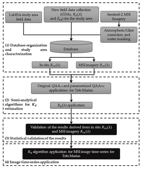
Figure 1. Materials and methods flowchart. LabISA stands for Instrumentation Laboratory for Aquatic Systems (in Portuguese).

2.1. Study Area

The study area consists of the Três Marias (TM) hydroelectric reservoir located in the upper valley of the São Francisco River, in the central region of Minas Gerais state (Figure 2) [1,2]. Constructed in 1957 and operating since 1962, TM reservoir is approximately 100 km long in its main axis along the São Francisco River and has a volume of at least 20 billion m³ of water [3]. Moreover, the TM reservoir has clear water characteristics, except at the entrance of its tributaries and the banks due to its shallow depth favoring sediment resuspension and bottom effect transparency measurements [28,29]. TM reservoir watershed is characterized by a humid tropical climate with average annual rainfall precipitation of 1400 mm of [30] concentrated between October and March (85%) [31]. Most of its watershed is inside the Cerrado biome (Brazilian Savannah), with some fragments of the Mata Atlântica biome (Atlantic Forest) [32]. The main rivers feeding TM reservoir are São Francisco, Pará, and Paraopeba Rivers (Figure 2a) [33]. Furthermore, TM watershed main land uses and land cover consist of cattle grazing, patches of the Atlantic forest, urban areas, and a relevant mining industry activity [32].

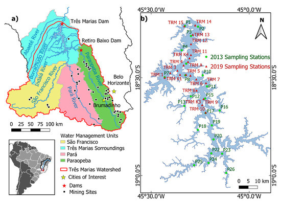
Figure 2. Study area: (a) Três Marias drainage basin; and (b) 2013 and 2019 sampling stations.

Most of the mining sites inside TM watershed are located within Paraopeba and Pará Rivers sub-basins. Most of them are located along the Paraopeba River, with particular attention to the region between Brumadinho city and Belo Horizonte Metropolitan Region, and Pará River sub-basin (Figure 2a). This area suffered a huge disaster related to the breaking of a mining tailings dam in Brumadinho city on the 25 January 2019, which caused at least 259 deaths [34]. This event highlighted the importance of the Paraopeba river since it drains all the runoff waters from Brumadinho city and part of the Belo Horizonte Metropolitan Region [32,35].

The water transparency and the trophic state of the TM reservoir show seasonal changes with lower concentrations of $chla$ and TSS during the dry season [8,10,36]. Generally, the TM reservoir waters are more transparent in the middle of its main channel, having the lowest transparencies at the entrances of its main tributaries. In general, São Francisco River waters that flow into the TM have higher TSS concentrations and lower transparency than those of Paraopeba River [37]. This difference may be explained by the existence of a small-scale reservoir (Retiro Baixo) just upstream of the Paraopeba River entrance that holds part of the sediments which, otherwise would be transported into TM reservoir.

2.2. Field Data Acquisition

Data collection was carried out at 42 sampling stations (see Figure 2b): 22 from 17–22 June 2013; and 20 from 30 June to 2 July 2019.

Radiometric data were acquired using inter-calibrated TriOS-RAMSES radiometers (Rastede, Germany) to measure $L_t\left(\mathsf{\theta };\mathsf{\varphi };\mathsf{\lambda }\right)$, $L_{sky}\left(\mathsf{\theta }\prime ;\mathsf{\varphi };\mathsf{\lambda }\right)$, $E_s\left(\mathsf{\lambda }\right)$ and $E_d\left(\mathrm{z};\mathsf{\lambda }\right)$, within 350–900 nm wavelength range. The framework for the four radiometers (Figure 3) was: (i) $L_w\left(\mathsf{\lambda }\right)$ within a nadir angle ($\mathsf{\theta }$) of 45° and Sun azimuth angle ($\mathsf{\varphi }$) of 135°; (ii) $L_{sky}\left(\mathsf{\lambda }\right)$ within a zenithal angle ($\mathsf{\theta }\prime$) of 45° and azimuthal angle of 135°; (iii) $E_s\left(\mathsf{\lambda }\right)$ at 180° in relation to the water surface; and, (iv) $E_d\left(\mathrm{z};\mathsf{\lambda }\right)$ positioned in a cage and submerged with the aid of a crane. The above-water sensors were positioned 2 m away from the water surface to avoid shadow and vessel reflections. This acquisition geometry is based on Mobley [38] to avoid glint effects.

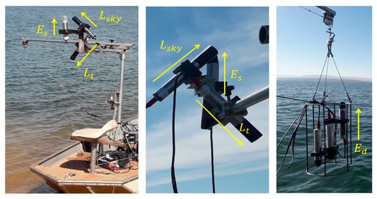
Figure 3. Field radiometric measurements framework scheme.

The total absorption coefficient $a\left(\mathsf{\lambda }\right)$ was measured with the Wetlabs Spectral Absorption and Attenuation meter (ACS, Bellevue, United States) [39] during the 2013 campaign, while in 2019, it was determined in the laboratory as described in Section 2.3.

Water sampling collection protocols followed the American Public Health Association (APHA) [40]. Water samples were collected at approximately 30 cm of depth using sampling bottles coated with opaque material and then stored inside a cooler with ice until its filtration. After the samples collection, the filtration was conducted to prepare the water samples and the filters for laboratory analysis and determination of $chla$, TSS, $a_{CDOM}\left(\mathsf{\lambda }\right)$, $a_p\left(\mathsf{\lambda }\right)$, and its fractions $a_{\mathsf{\varphi }}\left(\mathsf{\lambda }\right)$ and $a_d\left(\mathsf{\lambda }\right)$. Filter Whatman GF/F was used for chla, $a_p\left(\mathsf{\lambda }\right)$, and its fractions $a_{\mathsf{\varphi }}\left(\mathsf{\lambda }\right)$ and $a_d\left(\mathsf{\lambda }\right)$, and Whatman GF/C for TSS, while water samples filtered using Nylon filters with pore diameter of 0.22 µm were used for CDOM. The chla and TSS samples were frozen inside envelopes at temperatures below 0°C, while $a_p\left(\mathsf{\lambda }\right)$ and fractions samples were frozen inside opaque vials in a liquid nitrogen bottle at temperatures below −196 °C. The CDOM water samples were chilled without freezing it.

2.3. Spectral and Water Quality Field Data

2.3.1. Optically Active Constituents

The $chla$ concentration was determined using the Nush method [41] based on the 665 and 750 nm absorbances read in a spectrophotometer (brand Agilent/Varian, model Cary-50 Conc, Santa Clara, United States). This method extracts the phytoplankton pigments retained in the Whatman GF/F filter by warm ethanol followed by a thermal shock. The extracted pigments were put to rest for 6 to 24 h inside a fridge protected from light before the measurements. Finally, sample extractions were read in the spectrophotometer using quartz cuvettes with 50 mm of the optical path.

TSS concentrations were computed using pre-calcined and pre-weighed Whatman GF/C filters. Before laboratory analysis, the filters were thawed in the laboratory and dried using a laboratory drying-oven. After that, dried filter samples were weight-measured using a precision scale [42] in a room with controlled air conditions. Finally, the concentrations were calculated using the relation between the filter retained solid weight and the volume of filtered water samples [42].

2.3.2. Apparent Optical Properties

The AOP parameters derived from the radiometric field measurements used in this study were the $R_{rs}\left(\mathsf{\lambda }\right)$ and $K_d\left(\mathsf{\lambda }\right)$. The Remote Sensing Reflectance was calculated using Equation (1).

$$R_{rs}\left(\mathsf{\theta };\mathsf{\varphi };\mathsf{\lambda }\right)=\frac{L_t\left(\mathsf{\theta };\mathsf{\varphi };\mathsf{\lambda }\right)-\rho L_{sky}\left(\mathsf{\theta }\prime ;\mathsf{\varphi };\mathsf{\lambda }\right)}{E_s\left(\mathsf{\lambda }\right)},$$

(1)

where $\rho \left(\mathsf{\theta };\mathsf{\varphi }\right)$ is the reflectance factor at the air-water interface. The values for each field station were obtained from Mobley [38] Look-Up-Table, based on in-situ wind speed and geometry acquisition. For each sample station, around 150 measurements of $L_t\left(\mathsf{\theta };\mathsf{\varphi };\mathsf{\lambda }\right)$, $L_{sky}\left(\mathsf{\theta }\prime ;\mathsf{\varphi };\mathsf{\lambda }\right)$ and $E_s\left(\mathsf{\lambda }\right)$ were obtained. At each field station, the representative spectrum was determined by the closest to the median spectrum, as described in Maciel et al. [43].

The Diffuse Attenuation Coefficient ($K_d$) was computed from the profiles of downwelling planar irradiance ($E_d$) measured at each station. The $E_d\left(\mathsf{\lambda }\right)$ measurements were acquired by submerging the equipment up to the euphotic depth (1% of the subsurface $E_d$) at the wavelength of maximum penetration. Therefore, Equation (2) summarizes the propagation of $E_d\left(\mathsf{\lambda }\right)$.

$$E_d\left({\mathrm{z}}_{\mathrm{m}};\mathsf{\lambda }\right)=E_d\left(z_1;\mathsf{\lambda }\right) e^{-K_d\left(\mathsf{\lambda }\right)z},$$

(2)

where $E_d\left({\mathrm{z}}_{\mathrm{m}};\mathsf{\lambda }\right)$ represents the downwelling irradiance measured at the depth (${\mathrm{z}}_{\mathrm{m}}$), and $E_d\left(z_1;\mathsf{\lambda }\right)$ is the subsurface downwelling irradiance (the first measurement used to calculate $K_d\left(\mathsf{\lambda }\right)$). Due to the variability in $E_s\left(\mathsf{\lambda }\right)$ values related to changes in cloud cover and solar angle, $E_d\left({\mathrm{z}}_{\mathrm{m}};\mathsf{\lambda }\right)$ was normalized ($E{\prime }_d\left({\mathrm{z}}_{\mathrm{m}};\mathsf{\lambda }\right)$) by $E_s\left(\mathsf{\lambda }\right)$ [44]. This normalization followed the protocols of Mueller [23], calculating $E{\prime }_d\left({\mathrm{z}}_{\mathrm{m}};\mathsf{\lambda }\right)$ by multiplying $E_d\left({\mathrm{z}}_{\mathrm{m}};\mathsf{\lambda }\right)$ by a Normalization Factor ($NF\left({\mathrm{z}}_{\mathrm{m}},\mathsf{\lambda }\right)$) (Equation (3)).

$$E{\prime }_d\left({\mathrm{z}}_{\mathrm{m}};\mathsf{\lambda }\right)=E_d\left({\mathrm{z}}_{\mathrm{m}};\mathsf{\lambda }\right) NF\left({\mathrm{z}}_{\mathrm{m}},\mathsf{\lambda }\right)=\frac{E_d\left({\mathrm{z}}_{\mathrm{m}};\mathsf{\lambda }\right) E_s\left(t\left(z_1\right),\mathsf{\lambda }\right)}{E_s\left(t\left({\mathrm{z}}_{\mathrm{m}}\right),\mathsf{\lambda }\right)},$$

(3)

where $NF\left({\mathrm{z}}_{\mathrm{m}},\mathsf{\lambda }\right)$ is the ratio between the first measurement of $E_s\left(\mathsf{\lambda }\right)$ (at the same instant of the $E_d\left(z_1;\mathsf{\lambda }\right)$) by $E_s\left(\mathsf{\lambda }\right)$ measurement concomitant with $E_d\left({\mathrm{z}}_{\mathrm{m}};\mathsf{\lambda }\right)$. Therefore, $K_d\left(\mathsf{\lambda }\right)$ can be calculated through Equation (4) using $E{\prime }_d\left({\mathrm{z}}_{\mathrm{m}};\mathsf{\lambda }\right)$. $K_d\left(\mathsf{\lambda }\right)$ is given by the straight-line slope that passes through the origin (i.e., the slope of the relationship of Equation (4)). Only points resulting in R² higher than 0.98 were used for $K_d\left(\mathsf{\lambda }\right)$ computation, as observed by Mishra et al. [44].

$$K_{d-measured}\left(z,\mathsf{\lambda }\right)=-\frac{1}{z_m-z_1} \ln \left[\frac{E{\prime }_d\left(z_m, \mathsf{\lambda }\right)}{E{\prime }_d\left(z_1, \mathsf{\lambda }\right)}\right],$$

(4)

From hereafter, $K_{d-measured}$ will represent the field measured $K_d\left(\mathsf{\lambda }\right)$.

2.3.3. Inherent Optical Properties

CDOM water samples were read using a UV/VIS spectrophotometer (brand Shimadzu, model UV2600, Kyoto, Japan). Spectrophotometer readings were preprocessed to subtract the mean value of the measurements of spectral absorbance (A(λ)) and offset [45,46], and then transformed into $a_{CDOM}\left(\mathsf{\lambda }\right)$ [47] using a relationship between A(λ) and the cuvette optical path length ($l$) (Equation (5)).

$$a_{CDOM}\left(\mathsf{\lambda }\right)=2.3 \frac{A\left(\mathsf{\lambda }\right)}{l},$$

(5)

The measurements of $a\left(\mathsf{\lambda }\right)$ using ACS equipment, during the 2013 campaign, were acquired for the water column profile at each sampling station [29]. The data were smoothed to eliminate the measurement noise. Since the water column was not stratified in most of the sampling stations, the median of the $a\left(\mathsf{\lambda }\right)$ profile was used to represent $a\left(\mathsf{\lambda }\right)$ for the whole water column.

Finally, to assess $a_p\left(\mathsf{\lambda }\right)$, and its fractions ($a_d\left(\mathsf{\lambda }\right)$ and $a_{\mathsf{\varphi }}\left(\mathsf{\lambda }\right)$) for the 2019 campaign, Whatman GF/F filters with retained material were analyzed using the UV/VIS spectrophotometer (Shimadzu UV2600) with dual-beam and an integrating sphere following the methodology proposed by Tassan & Ferrari [48,49]. Measurements of optical density (OD) were determined and corrected for the particulate material to estimate $a_p\left(\mathsf{\lambda }\right)$ in the first reading [49,50]. After that, the pigments in the filter were leached with sodium chloride and then read again to determine the detritus corrected OD and estimate $a_d\left(\mathsf{\lambda }\right)$ [49,50]. This approach measures the spectral reflectance and transmittance to estimate the $a_p\left(\mathsf{\lambda }\right)$ and $a_d\left(\mathsf{\lambda }\right)$, and then $a_{\mathsf{\varphi }}\left(\mathsf{\lambda }\right)$ by subtracting $a_d\left(\mathsf{\lambda }\right)$ from the $a_p\left(\mathsf{\lambda }\right)$ [42,48,49].

2.4. Sentinel-2 MSI Data

MultSpectral Imager (MSI) images from Sentinel-2 A and B were used in the useful spectral range for assessing water transparency (Table 2) including the visible (B2 to B5) and near-infrared (B6 and B8) bands, and the shortwave infrared region (B11) needed for glint effect correction [51,52]. These images were used to assess temporal changes in $K_d$, resulting from both natural processes and impacts of the Brumadinho disaster on TM reservoir.

Table 2. Sentinel-2MSI spectral bands used in this study.

Band (Spatial Resolution)	Central Wavelength (nm)	Bandwidth (nm)	SNR 1
B2 (10 m)	492 (Blue)	98	154
B3 (10 m)	560 (Green)	45	168
B4 (10 m)	665 (Red)	38	142
B5 (20 m)	704 (Red Edge)	19	117
B6 (20 m)	741 (Red Edge)	18	89
B8 (10 m)	833 (IVP)	145	174
B11 (20 m)	1614 (SWIR)	91	100

¹ SNR: Signal to noise ratio calculated in laboratory data for reference radiance of each band [53].

2.5. Kd(λ) Semi-Analytical Algorithm

In this study, we used the relationship between the diffuse attenuation coefficient ($K_d$) and IOPs [54,55] to reparametrize and apply a semi-analytical algorithm of $K_d\left(\mathsf{\lambda }\right)$ ($K_{d-SA}\left(\mathsf{\lambda }\right)$—Equation (6)) to our study site, using $a\left(\mathsf{\lambda }\right)$ and $b_b\left(\mathsf{\lambda }\right)$ data as input [26]. From hereafter, the semi-analytical $K_d\left(\mathsf{\lambda }\right)$ will be named as $K_{d-SA}$.

$$K_{d-SA}\left(\mathsf{\lambda }\right)=\left(1+m_0 {\mathsf{\theta }}_s\right)a\left(\mathsf{\lambda }\right)+\left(1-\gamma {\mathsf{\eta }}_w\left(\mathsf{\lambda }\right)\right) m_1\left(1-m_2 \left(e^{-m_3 a\left(\mathsf{\lambda }\right)}\right)\right)b_b\left(\mathsf{\lambda }\right),$$

(6)

where, m₀, m₁, m_2, and m₃ are constants independent from wavelength and water type, ${\mathsf{\theta }}_s$ is the zenithal sun angle, $\gamma$ a parameter that represents the effect caused by the variation in the scattering constituents in the water, and ${\mathsf{\eta }}_w\left(\mathsf{\lambda }\right)$ the parameter that quantifies the contribution of $b_{bw}\left(\mathsf{\lambda }\right)$ over the total $b_b\left(\mathsf{\lambda }\right)$ (Equation (7)).

$${\mathsf{\eta }}_w\left(\mathsf{\lambda }\right)=b_{bw}\left(\mathsf{\lambda }\right)/b_b\left(\mathsf{\lambda }\right),$$

(7)

$K_{d-SA}\left(\mathsf{\lambda }\right)$ was used with Lee et al. [26] original values for $m_0$, $m_1$, $m_2$, $m_3$ and $\gamma$ (0.005, 4.259, 0.52, 10.8 m and 0.265 respectively), while ${\mathsf{\theta }}_s$ was calculated using the geographic coordinates, day of the year, and hour of data acquisition.

2.5.1. Deriving Inherent Optical Properties from Remote Sensing Reflectance

To derive $a\left(\mathsf{\lambda }\right)$ and $b_b\left(\mathsf{\lambda }\right)$ as input for equation 6, the empirical steps of the original QAA in its version 6 (QAAv6) [24,56] were reparametrized using ${\mathsf{\lambda }}_0$, the reference wavelength, at 560 nm (although the use of ${\mathsf{\lambda }}_0=670 \mathrm{nm}$ in the original QAAv6 (Table 3—steps 2 and 4).

Table 3. Summary of QAA_TM Description and original QAAv6 steps.

# 1	QAATM 2	QAAv6 3 [56]
1	The same as the QAAv6, where the $r_{rs}\left(\lambda \right)$ is derived analytically from $R_{rs}\left(\mathsf{\lambda }\right)$; $u\left(\lambda \right)$ can be explained from the relation between $a\left(\lambda \right)$ and $b_b\left(\lambda \right)$, and derived from $r_{rs}\left(\lambda \right)$, $g_0$ and $g_1$ values.	$r_{rs}\left(\mathsf{\lambda }\right)=\frac{R_{rs}\left(\mathsf{\lambda }\right)}{\left(0.52+1.7 R_{rs}\left(\mathsf{\lambda }\right)\right)}$ $r_{rs}\left(\mathsf{\lambda }\right)=g_{0}u\left(\lambda \right)+g_0{\left[u\left(\lambda \right)\right]}^2$ $u\left(\lambda \right)=\frac{b_b\left(\lambda \right)}{\left(a\left(\lambda \right)+b_b\left(\lambda \right)\right)}$ $u\left(\lambda \right)=-\frac{g_0+\sqrt{\left[g_0^2+4 g_1 r_{rs}\left(\lambda \right)\right]}}{2 g_1}$ $g_0=0.089 \mathrm{e} g_1=0.1245$
2	Reparametrizated for MSI bands, choosing the best three bands ratio for this case.	$$\begin{gathered} a({\mathsf{\lambda }}_0{}^4) \\ =a_w\left({\mathsf{\lambda }}_0\right)+0.39{\left(\frac{R_{rs}\left({\mathsf{\lambda }}_0\right)}{R_{rs}\left(443\right)+R_{rs}\left(490\right)}\right)}^{1.14} \end{gathered}$$
3	From $a\left({\mathsf{\lambda }}_0\right)$ determined in step 2, the $b_{bp}\left({\mathsf{\lambda }}_0\right)$ was then derived.	$b_{bp}\left({\mathsf{\lambda }}_0\right)=\frac{u\left({\mathsf{\lambda }}_0\right) a\left({\mathsf{\lambda }}_0\right)}{1-u\left({\mathsf{\lambda }}_0\right)}-b_{bw}\left({\mathsf{\lambda }}_0\right)$
4	Reparametrizated using the linearization of step 5 to derive $\eta$ values	$\eta =2\left(1-1.2\exp \left(-0.9\frac{r_{rs}\left(443\right)}{r_{rs}\left(555\right)}\right)\right)$
5	The same as the QAAv6.	$b_b\left(\lambda \right)=b_{bp}\left({\mathsf{\lambda }}_0\right){({\mathsf{\lambda }}_0/\mathsf{\lambda })}^{\eta }+b_{bw}\left(\lambda \right)$
6	The same as the QAAv6.	$a\left(\lambda \right)=\left(1-u\left(\mathsf{\lambda }\right)\right) \left(b_{bw}\left(\lambda \right)+b_{bp}\left(\lambda \right)\right)/u\left(\mathsf{\lambda }\right)$

¹ QAA steps used in this study; ² Lee QAAv6 description for TM reparametrization; ³ Lee original non-reparametrized QAAv6 [56]; ⁴ QAAv6 original ${\mathsf{\lambda }}_0=670 \mathrm{nm}$.

We named this reparametrized QAA as QAA_TM. For this reparametrization, only $a\left(\mathsf{\lambda }\right)$ derived from ACS [39] measurements carried out during the 2013 campaign (n = 22) were used as no ACS measurements were available for the 2019 campaign.

For empirical step 2, an exponential adjustment was carried out between $a\left({\mathsf{\lambda }}_0=560\right)$, derived from ACS, and a three-band ratio to derive the parameters M and N (Equation (8)). The wavelengths used in adjusting correspond to the central wavelength of MSI B3, B4, and B5 bands [57]. The $R_{rs}$ used in the bands ratio were derived from in situ measurements at each of the 22 sampling stations.

$$a\left(560\right)=a_w\left(560\right)+M\ast {\left(\frac{R_{rs}\left(560\right)}{R_{rs}\left(665\right)+R_{rs}\left(704\right)}\right)}^N,$$

(8)

To reparametrize the second empirical step (step 4 of QAAv6) [34], first $b_{bp}\left(\mathsf{\lambda }\right)$ was obtained from $a\left(\mathsf{\lambda }\right)$, derived from ACS field measured at sampling station of the 2013 campaign (Equation (9)), and then, knowing $b_{bp}\left(\mathsf{\lambda }\right)$, a linear fitting was applied to step 5 of QAAv6 (Equation (10)) to estimate the power value η for each sampling station [57].

$$b_{bp}\left(\mathsf{\lambda }\right)=\frac{u\left(\mathsf{\lambda }\right) a\left(\mathsf{\lambda }\right)}{1-u\left(\mathsf{\lambda }\right)}-b_{bw}\left(\mathsf{\lambda }\right),$$

(9)

$$\ln \left[b_{bp}\left(\mathsf{\lambda }\right)\right]=\mathsf{\eta }\ln \left(\frac{{\mathsf{\lambda }}_0}{\mathsf{\lambda }}\right)+\ln \left[b_{bp}\left({\mathsf{\lambda }}_0\right)\right],$$

(10)

where $u\left(\mathsf{\lambda }\right)$ is the ratio of $b_b$ to ($a+b_b$) derived from subsurface remote sensing reflectance ($r_{rs}\left(\mathsf{\lambda }\right)$) using QAA step 1 equation [24,56] (Table 3), and $b_{bw}$ is the backscattering coefficient of pure water [58].

To obtain η from $r_{rs}$, similarly to step 4 of QAAv6, we adjusted Equation (11), based on the stations η derived from Equation (10) and a two-band ratio using the central wavelength of MSI B4 and B5 bands.

$$\mathsf{\eta }=A e^{\frac{r_{rs}\left(665\right)}{r_{rs}\left(704\right)}}+B,$$

(11)

Finally, the parametrized QAA_TM was applied using $R_{rs}\left(\mathsf{\lambda }\right)$ data to compute $a\left(\mathsf{\lambda }\right)$ and $b_b\left(\mathsf{\lambda }\right)$ used as input for $K_{d-SA}$.

2.5.2. Semi-Analytical Algorithm Validation

The reparametrized semi-analytical algorithm $K_{d-SA}\left(\mathsf{\lambda }\right)$ was applied and validated using two datasets as input: (i) first with the in situ $R_{rs}\left(\mathsf{\lambda }\right)$ data; and then, (ii) with the $R_{rs}\left(\mathsf{\lambda }\right)$ derived from MSI image bands.

Both $K_{d-SA}\left(\mathsf{\lambda }\right)$ derived from in situ $R_{rs}\left(\mathsf{\lambda }\right)$ and $K_{d-SA}\left(\mathsf{\lambda }\right)$ derived from MSI Sentinel-2 A image, acquired in 1 July 2019 coincident with in situ samplings, were validated with 20 sampling stations of 2019 campaign. The validations were performed from blue to red MSI bands (B1 to B4) for each dataset.

Since the MSI revisit time is 5 days, we used an image covering TM in the middle of the 2019 campaign (1 July). For this reason, the in situ measurements may differ up to 1 day from the satellite image. This difference should not be of great concern because there was no rainfall precipitation during the survey campaign, which could change the OACs.

For each algorithm and each dataset, the estimated $K_{d-SA}\left(\mathsf{\lambda }\right)$ was compared with $K_{d-measured}\left(\mathsf{\lambda }\right)$ using a linear regression approach to assess algorithm accuracy (Section 2.6). The reparametrized QAA_TM algorithm was applied to the MSI image time series, as shown in Section 2.7.

2.6. Data Analysis and Accuracy Assessment

For the validation of $K_{d-SA}$ algorithm, the $K_{d-measured}$ was used as a reference and the following statistical metrics were calculate for performance evaluation: correlation coefficient (R²—Equation (12)); the mean absolute percentage error (MAPE—Equation (13)); and, the Root-Mean Square Error (RMSE—Equation (14)).

$$R^2=1-\frac{{{\displaystyle \sum }}_{i=1}^n{\left(y_i-{\widehat{y}}_i\right)}^2}{{{\displaystyle \sum }}_{i=1}^n{\left(y_i-{\overline{y}}_i\right)}^2},$$

(12)

$$MAPE=\frac{100}{n} {{\displaystyle \sum }}_{i=1}^n\left|\frac{y_i-{\widehat{y}}_i}{y_i}\right|,$$

(13)

$$RMSE=\sqrt{\frac{{{\displaystyle \sum }}_{i=1}^n{\left(y_i-{\widehat{y}}_i\right)}^2}{n}},$$

(14)

where, $y_i$ is the reference field value, ${\widehat{y}}_i$ the predicted value, ${\overline{y}}_i$ the average of the field reference value, and n the size of the dataset. All the linear regressions and the accuracy assessment for the validations were done based on the MSI bands B1 to B5 wavelengths.

2.7. Time Series Kd Algorithm Application

The most accurate algorithm was applied to a 2017–2019 time series of Sentinel-2 A and B imagery for mapping time changes in TM spectral $K_{d-SA}\left(\mathsf{\lambda }\right)$. Moreover, images with less than 10% of cloud cover over the scene were used in the query searches to reduce the data volume.

First, the image collection was downloaded and preprocessed (Section 2.7.1). After the preprocessing, the $K_{d-SA}\left(\mathsf{\lambda }\right)$ the algorithm was applied to the image dataset and then monthly-average filtered.

Finally, the results for the time series were extracted for three sampling points distributed along reservoir mean inflow and outflow rates for each month of the period. Eventually, months without images following the pre-requirements were not used, causing gaps in the time series.

2.7.1. Sentinel-2 MSI Time Series Preprocessing

First, the image dataset was loaded from the internet and processed using an internal algorithm from the Instrumentation Laboratory of Aquatic Systems (LabISA) that downloads the images at the top of the main axis of TM reservoir (downstream, middle, and upstream) using Quantum GIS software. The extracted results were confronted with the accumulated rainfall precipitation for the watershed and the atmosphere level (L1C) from Google Earth Engine API, then applies AtmosPy atmospheric correction algorithm [59] achieving surface level (L2C). AtmosPy is a processing interface to run the Second Simulation of the Satellite Signal in the Solar Spectrum (6S–6SV) atmospheric correction algorithm [60,61]. In the Atmospy interface, the 6S algorithm receives atmospheric products from Multi-Angle Implementation of Atmospheric Correction (MAIAC) like water vapor, ozone, and aerosol optical depth. After atmospheric correction, the LabISA routine applies the fmask algorithm [62] to produce a water mask without clouds and cloud shades.

After atmospheric correction and masking, the image dataset was standardized to 10 m by resampling bands B5, B6, and B11 using the nearest neighbor method to match VIS bands’ spatial resolution. Finally, the glint effect was removed, subtracting the band B11 values from all the remaining five bands [51].

3. Results

3.1. In Situ Limnology Data

The subsurface $chla$ and TSS concentrations, and the $Z_{sd}$ measurements have different ranges for each campaign (Table 4). For the 2013 field campaign, $chla$ values varied from 1.17 to up to 13.22 mg m⁻³ with a mean value of 5.27 mg m⁻¹ while for 2019, the values varied between 1.33 and 7.95 mg m⁻³ with the mean value of 3.66 mg m⁻³. On the other hand, TSS values were more homogeneous between these campaigns (mean of 3.66 and 2.77 g m⁻³ for 2013 and 2019, respectively). Similar to $chla$ and TSS, the Secchi disk depth ($Z_{sd}$) also showed higher variability for the 2013 campaign as opposed to that of 2019 one. These values were distinct, even for nearby stations between the campaigns.

Table 4. Summary for $chla$, TSS and $Z_{sd}$ values statistics.

Parameter	2013
	Range 1	Mean 2	Median 3	CV 4	SD 5
$chla$	1.17–13.22	5.27	4.46	64.37	3.39
TSS	1.33–7.95	3.66	3.32	44.56	1.63
$Z_{sd}$	0.50–4.62	2.32	2.12	41.35	0.96
Parameter	2019
	Range	Mean	Median	CV	SD
$chla$	0.42–5.70	2.53	2.41	53.74	1.36
TSS	0.70–6.67	2.77	2.30	55.93	1.55
$Z_{sd}$	2.81–4.42	3.62	3.58	12.44	0.42

¹ Range of concentration; ² Concentration mean; ³ Concentration median; ⁴ Coefficient of variation [%]; ⁵ Standard deviation in concentration unit.

The descriptive statistics of $chla$, TSS, and $Z_{sd}$ variation for each campaign are in Table 4.

3.2. In Situ Radiometric Characterization

3.2.1. Apparent Optical Properties

Field $R_{rs}\left(\mathsf{\lambda }\right)$ values showed higher amplitudes for the 2013 campaign (Figure 4a) than those for 2019 (Figure 4b), highlighting P25 and P26 stations during 2013 (Figure 2) with the highest $R_{rs}\left(\mathsf{\lambda }\right)$ values near 560 nm (Figure 4a–dotted lines). Both stations presented high TSS values (2.36 and 6.41 g m⁻³ respectively), and low $Z_{sd}$ values (0.85 and 0.50 m respectively). In general, $R_{rs}\left(\mathsf{\lambda }\right)$ peaks have occurred in the green region of the spectrum (between 550 to 580 nm) reaching values from 0.005 up to 0.042 sr⁻¹, and two other little “shoulders” in the red region, one at 620 nm and the other between 676 and 679 nm, approximately. Moreover, the $R_{rs}\left(\mathsf{\lambda }\right)$ in the NIR region (700 to 750 nm) were the lowest ones, reaching null (0) values.

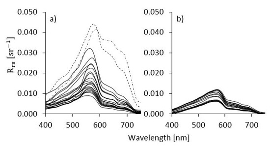
Figure 4. Field $R_{rs}\left(\mathsf{\lambda }\right)$ values for: (a) 2013; and, (b) 2019.

For the $K_{d-measured}$ calculation, it is necessary to understand the $E_d\left(\mathrm{z};\mathsf{\lambda }\right)$ decay as the water column depth increases. Figure 5 presented one example of E_d profile in the water column, in a logarithmic scale, for each campaign for blue (443 nm), green (560 nm), and red (665 nm) wavelengths. For both campaigns, the highest light attenuation occurred at 443 nm, when it reached 1% of the subsurface $E_d\left(\mathrm{z};\mathsf{\lambda }\right)$ at approximately 6 m depth. The red region followed the blue region with penetration of approximately 7 m of the subsurface $E_d\left(\mathrm{z};\mathsf{\lambda }\right)$ at 665 nm. Finally, the highest light penetration occurred at 560 nm (green) with approximately 13 m of euphotic depth.

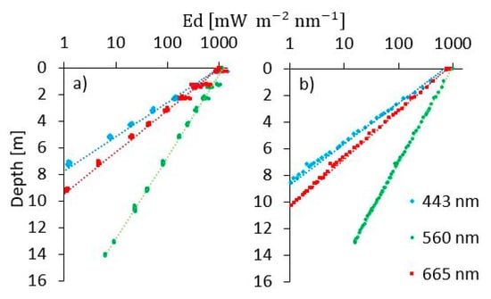
Figure 5. Examples of linear profiles for logarithm scale of $E_d\left(\mathrm{z};\mathsf{\lambda }\right)$: (a) P15 2013; and, (b) TRM09 2019.

The spectral decay of $E_d\left(\mathrm{z};\mathsf{\lambda }\right)$ with depth in the water column (Figure 5) was used to calculate the $K_{d-measured}\left(\mathsf{\lambda }\right)$ (Figure 6). According to in-situ limnology and $R_{rs}$ data, higher $K_{d-measured}\left(\mathsf{\lambda }\right)$ values were observed for the 2013 campaign. The $K_{d-measured}\left(\mathsf{\lambda }\right)$ in the blue region (< 500 nm) reached up to approximately 1.5 m⁻¹ at 443 nm. Moreover, 2013 data also presented a high range of values compared to those of the 2019 campaign, which is clearly due to the high variability in field-measured OACs. It is also important to highlight that stations P25 and P26 (Figure 6—Dotted lines) presented uncertainties in $K_{d-measured}\left(\mathsf{\lambda }\right)$ for wavelengths lower than 500 nm, which can be attributed to high CDOM and TSS absorption at those wavelengths [63].

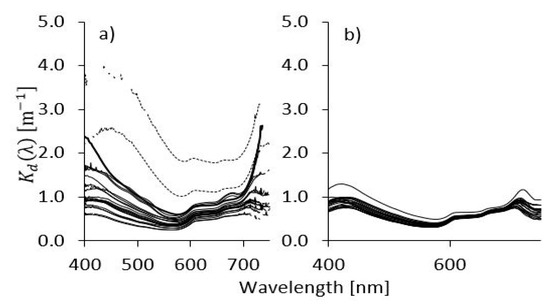
Figure 6. Field $K_d\left(\mathsf{\lambda }\right)$ for: (a) 2013; and, (b) 2019.

Similar to the $E_d\left(\mathrm{z};\mathsf{\lambda }\right)$ decay (Figure 5), Figure 6 shows that the water column light penetration was higher in the green region of the spectrum (550–600 nm) for all stations, which is represented by $K_{d-measured}\left(\mathsf{\lambda }\right)$ lower values.

3.2.2. Inherent Optical Properties

The measurements of in-situ total absorption coefficient ($a\left(\mathsf{\lambda }\right))$ values (Figure 7) followed the observed results for $R_{rs}$ and limnological data. Note that for 2013 the $a\left(\mathsf{\lambda }\right)$ were acquired through ACS measurements whereas for 2019 $a\left(\mathsf{\lambda }\right)$ data were obtained through a spectrophotometer (See Section 2.2.). Besides, when both were compared, the results follow the same pattern. All $a\left(\mathsf{\lambda }\right)$ spectra showed $chla$ absorption features at approximately 676 to 679 nm wavelengths. From Figure 7 it is possible to note that the lowest $a\left(\mathsf{\lambda }\right)$ occurred at 550–580 range, following that observed for $K_d$. Moreover, one can note that as the wavelength increases the contribution of pure water absorption ($a_w\left(\mathsf{\lambda }\right)$) increases in the total $a\left(\mathsf{\lambda }\right)$, (Figure 7—Red-dotted line), with approximately 80% in the red domain (665 nm) and with almost 100% at wavelengths higher than 700.

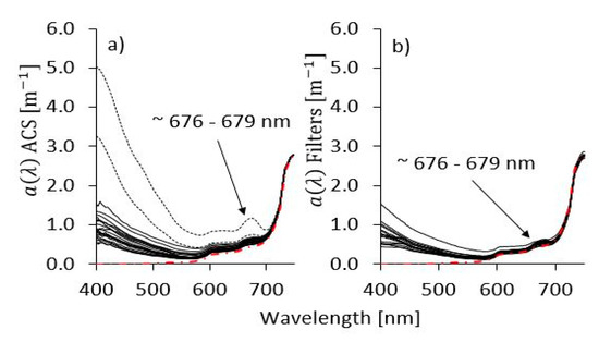
Figure 7. Field $a\left(\mathsf{\lambda }\right)$ values for: (a) 2013; and, (b) 2019.

For CDOM measurements, $a_{CDOM}\left(\mathsf{\lambda }\right)$ at 443 nm ($a_{CDOM}\left(443\right)$) (Figure 8) and spectral $a_{CDOM}\left(\mathsf{\lambda }\right)$ (Figure 8) achieved higher variation for the 2013 campaign (~0.1 to up to 0.8 m⁻¹) compared to the 2019 (~0.1–0.3 m⁻¹), mostly due to the stations inside TM main affluent rivers (P13, P23, P25, and P26), represented as blue dotted-lines in Figure 8a. Besides, these stations presented different slopes of CDOM decay, which can be attributed to different sources of organic matter from those tributaries. The $a_{CDOM}\left(443\right)$ statistical parameters (mean, median and standard deviation) for each campaign are in Figure 8.

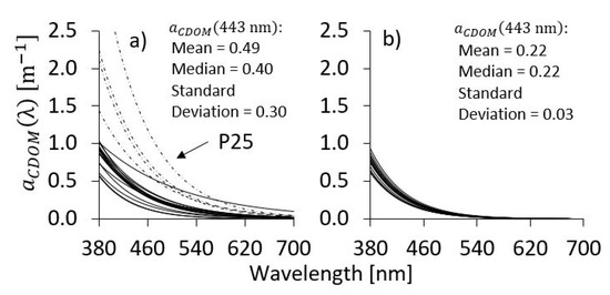
Figure 8. Field values for (a) 2013 $a_{CDOM}\left(\mathsf{\lambda }\right)$; and, (b) 2019 $a_{CDOM}\left(\mathsf{\lambda }\right)$.

Higher $a_{CDOM}\left(443\right)\mathrm{values}$ (Figure 8) were found at the sampling stations with higher $R_{rs}\left(\mathsf{\lambda }\right)$ (Figure 4) for wavelengths in the blue to green regions of the spectrum, between approximately 400 and 560 nm.

3.3. QAA_TM Parametrization

The exponential adjustment between $a\left(560\right)$ and the three bands $R_{rs}\left(560\right)/R_{rs}\left(665\right)+R_{rs}\left(704\right)$ (Figure 9a) showed good results, with R² of 0.93. Besides that, the linear adjustment between the $\mathsf{\eta }$ and the exponential of the two bands ratio $R_{rs}\left(665\right)/R_{rs}\left(704\right)$ (Figure 9b) produced R² of 0.41 for the same 22 sampling stations.

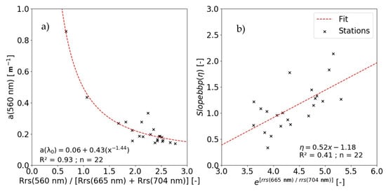
Figure 9. QAA_TM reparametrization: (a) step 2 exponential adjust; and, (b) step 4 linear adjust.

Nevertheless, the results from the estimation of the $\mathsf{\eta }$ by equation 10 used as preprocessing for step 4 reparametrization were satisfactory, with an average R² of 0.77. Table 5 summarizes the empirical steps of QAA_TM and QAA. The parametrized QAA_TM as the QAAv6 adapted for MSI bands used to derive $a\left(\mathsf{\lambda }\right)$ and $b_b\left(\mathsf{\lambda }\right)$ from $R_{rs}\left(\lambda \right)$ values are summarized in Table 5.

Table 5. Summary of QAA_TM and comparison with original QAAv6.

# 1	QAATM 2	QAA v6 3 [56]
2	$$\begin{gathered} a\left(560\right) \\ =a_w\left(560\right)+0.43{\left(\frac{R_{rs}\left(560\right)}{R_{rs}\left(665\right)+R_{rs}\left(704\right)}\right)}^{-1.44} \end{gathered}$$	$$\begin{gathered} a\left(665\right) \\ =a_w\left(665\right)+0.39{\left(\frac{R_{rs}\left(665\right)}{R_{rs}\left(443\right)+R_{rs}\left(492\right)}\right)}^{1.14} \end{gathered}$$
3	$b_{bp}\left(560\right)=\frac{u\left(560\right) a\left(560\right)}{1-u\left(560\right)}-b_{bw}\left(560\right)$	$b_{bp}\left(665\right)=\frac{u\left(670\right) a\left(665\right)}{1-u\left(665\right)}-b_{bw}\left(665\right)$
4	$\eta =0,5248\exp \left(\frac{r_{rs}\left(665\right)}{r_{rs}\left(704\right)}\right)$	$\eta =2\left(1-1.2\exp \left(-0.9\frac{r_{rs}\left(443\right)}{r_{rs}\left(560\right)}\right)\right)$
5	$b_b\left(\lambda \right)=b_{bp}\left(560\right){(560/\mathsf{\lambda })}^{\eta }+b_{bw}\left(\lambda \right)$	$b_b\left(\lambda \right)=b_{bp}\left({\mathsf{\lambda }}_0\right){(665/\mathsf{\lambda })}^{\eta }+b_{bw}\left(\lambda \right)$

¹ QAA steps with different parametrization for the algorithms; ² Lee QAAv6 parametrized for TM; ³ Lee original non-reparametrized QAAv6 [56].

3.4. In Situ $K_{d-SA}\left(\lambda \right)$ Validation

The QAA_TM (Figure 10a) showed better overall results for the spectral regions with the lowest $K_{d-SA}\left(\mathsf{\lambda }\right)$, agreeing most with the reference wavelength at 560 nm (B3). The results had excellent accuracy, with R² of 0.83, MAPE of 20.98%, and RMSE of 0.23 m⁻¹. Besides that, the results for the non-parametrized QAAv6 (Figure 10b) achieved R² of 0.68, MAPE of 21,20%, and RMSE of 0.18 m⁻¹, achieving better results around 665 nm (B4), used as the reference wavelength.

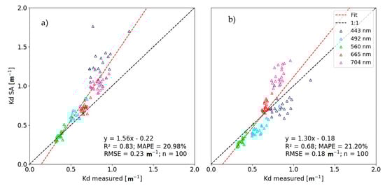
Figure 10. Global results for $K_d\left(\mathsf{\lambda }\right)$ derived from field $R_{rs}\left(\mathsf{\lambda }\right)$ measurements for: (a) QAA_TM; and, (b) QAAv6.

Regarding the slope and offset of the linear regression, QAA_TM showed a steeper slope and slightly similar offset when compared to QAAv6 (Figure 10). The different reference wavelength used in each QAA approach has a visible interference in the slope of the regressions and the accuracy of the results for each chosen band. QAA_TM approach had better accuracies for the lower values of $K_{d-SA}\left(\mathsf{\lambda }\right)$, agreeing most with the bands at 492, 560 and 665 nm (B2 to B4), while it overestimates higher values of $K_d\left(\mathsf{\lambda }\right)$ at 443 and 704 nm (B1 and B5). Besides that, QAAv6 had a better agreement with values at 560 and 665 nm (B3 and B4), overestimating the results of $K_{d-SA}\left(\mathsf{\lambda }\right)$ at 443 and 492 nm and overestimating results at 704 nm (B5).

The results of $K_{d-SA}\left(\mathsf{\lambda }\right)$ were also statistically assessed from B1 to B4 (Figure 11) to compare QAA_TM accuracy with the non-parametrized QAAv6 accuracy. For QAA_TM, the results for bands B2 to B4 showed good accuracies (Figure 11a), with R² of 0.77, 0.80 and 0.27; MAPE of 15% and 9%; and RMSE of 0.11, 0.04 and 0.07 m⁻¹, for each band, respectively; while B1 showed lower accuracy with R² of 0.18, MAPE of 50% and RMSE of 0.45 m⁻¹. The accuracy results for the non-parametrized QAAv6 (Figure 11b) were worse when compared to those for QAA_TM, with R² values of 0.27, 0.79, 0.82, and 0.35; MAPE of 16, 23, 19, and 12%; and RMSE of 0.16, 0.14, 0.08, and 0.11 m⁻¹, for bands B1 to B4 respectively. These statistical results, slopes and offsets for each band linear regression (Figure 11) agree with the overall results shown in Figure 10 above. While QAA_TM showed better results for the band at 560 followed by 665 and 492 nm respectively, the QAAv6 showed better results for the band at 665, followed by 560 nm.

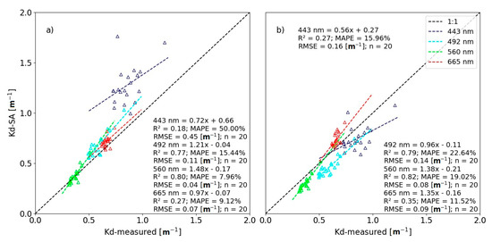
Figure 11. $K_{d-SA}\left(\mathsf{\lambda }\right)$ derived from field $R_{rs}\left(\mathsf{\lambda }\right)$ validations for: (a) QAA_TM at 443, 492, 560, and 665 nm; and, (b) validations for the original QAAv6 at 443, 492, 560, and 665 nm.

3.5. Satellite Validation

3.5.1. Glint Correction

After the glint effect removal from band B3 to B5 resulted in $R_{rs}$ more similar to those of the in situ $R_{rs}\left(\mathsf{\lambda }\right)$. Regarding bands B1 and B2, however, despite the improvement, Sentinel-2 $R_{rs}\left(\mathsf{\lambda }\right)$ were overestimated (Figure 12). Even after the glint removal most of the bands remained with significant errors in its values when compared with in situ measurements. The bands B3 (560 nm) and B4 (665 nm) achieved the best results after the glint removal, with R² of 0.90 and 0.82 and MAPE of 11 and 33%, respectively. While the results for bands B1 (443 nm), B2 (492 nm) and B5 (704 nm) achieved the worst results, with MAPE higher than 58% (Figure 12).

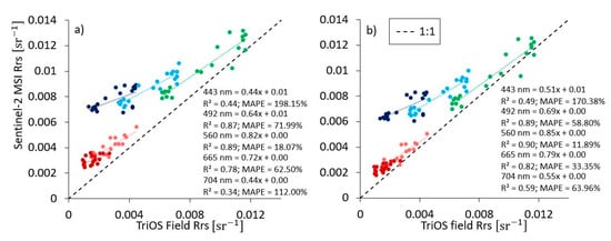
Figure 12. Comparison between Field $R_{rs}\left(\mathsf{\lambda }\right)$ and MSI $R_{rs}\left(\mathsf{\lambda }\right)$ for B1 to B5: (a) without glint removal; and, (b) with glint removal.

3.5.2. Sentinel-2 MSI $K_{d-SA}\left(\mathsf{\lambda }\right)$ Validation

Finally, the accuracy of $K_{d-SA}\left(\mathsf{\lambda }\right)$ derived from the MSI image was assessed for each band from B1 to B4 (Figure 13). QAA_TM results from band B1 to B3 showed the highest accuracies (Figure 13a), with R² of 0.43, 0.70 and 0.56; MAPE of 14, 14 and 38%; and RMSE of 0.14, 0.10 and 0.15 m⁻¹, for each band, respectively.

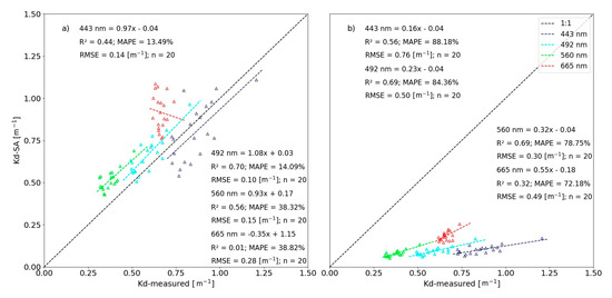
Figure 13. $K_{d-SA}\left(\mathsf{\lambda }\right)$ derived from MSI bands $R_{rs}\left(\mathsf{\lambda }\right)$ validations for (a) QAA_TM at 443, 492, 560, and 665 nm; and (b) QAAv6 at 443, 492, 560, and 665 nm.

Because there were images only from the 2019 campaign, the MSI image results were only validated for the stations measured that year.

The supplementary material of this paper includes the summary for the $K_{d-SA}\left(\mathsf{\lambda }\right)$ derived from MSI bands $R_{rs}\left(\mathsf{\lambda }\right)$ validations for QAAv6 (Figure S1).

3.5.3. Sentinel -2 MSI $K_{d-SA}\left(\mathsf{\lambda }\right)$ Time-Series

$K_{d-SA}\left(\mathsf{\lambda }\right)$ had the highest accuracies when using $b_b\left(\mathsf{\lambda }\right)$ and $a\left(\mathsf{\lambda }\right)$ derived from QAATM as input. Moreover, only the bands from B1 to B3 produced good statistical results, indicating that the approach combining QAATM plus $K_{d-SA}\left(\mathsf{\lambda }\right)$ should be applied only to these bands regarding the time series production. Figure 14 shows the monthly-averaged variation of $K_{d-SA}\left(\mathsf{\lambda }\right)$ for B2, the reservoir monthly-averaged inflow rate, and monthly-averaged outflow rate at the dam. $K_{d-SA}\left(\mathsf{\lambda }\right)$ refers to the Paraopeba River mouth, São Francisco River mouth, reservoir upper, middle and lower stream. $K_{d-SA}\left(\mathsf{\lambda }\right)$ time series showed a seasonal variation with higher values achieved during the rainy season for the assessed years (2017–2019).

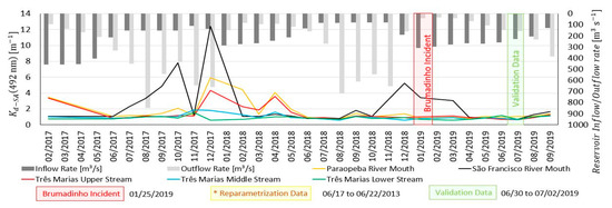
Figure 14. Monthly variation of average $K_{d-SA}\left(\mathsf{\lambda }\right)$ at MSI bands; monthly-averaged inflow and outflow rates for points at upper stream, middle stream, and lower stream regions of the reservoir. ^*, reparametrization data does not appear in the image time-series.

Generally $K_{d-SA}\left(492\right)$ highest values were found for the rainy period of the year (Figure 15), coinciding with the months with higher accumulated precipitations and higher monthly-averaged flow rates (October to March) [30].

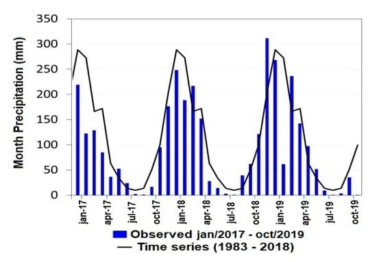
Figure 15. Monthly accumulated rainfall precipitation time series for Três Marias’s reservoir catchment. Source: Adapted from [30].

Representative $K_{d-SA}\left(492\right)$ results for two consecutive rainy and dry seasons are shown in Figure 16. During the dry season (Figure 16b,d), the $K_{d-SA}\left(492\right)$ is more spatially homogeneous, while for the rainy season (Figure 16a,c), higher gradients can be found, mostly at the entrance of the tributaries and in the upper portion of the reservoir.

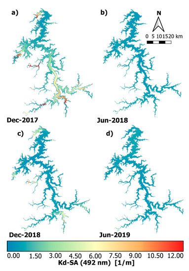
Figure 16. Examples of $K_d\left(492\right)$ for MSI time series: (a) December 2017; (b) June 2018; (c) December 2018; and, (d) June 2019.

4. Discussion

4.1. Algorithms Results Comparison

The ${\mathrm{K}}_{\mathrm{d}-\mathrm{SA}}\left(\mathsf{\lambda }\right)$ retrieved using IOPs derived from QAA_TM as input achieved better performance compared when using IOPs derived from QAAv6 for both in situ (Figure 11) and MSI (Figure 13) ${\mathrm{R}}_{\mathrm{rs}}\left(\mathsf{\lambda }\right)$ applicaiton. The linear regression at 492 nm for in situ data achieved slope factors of 1.21 and 0.96 for the QAA_TM and QAAv6 approaches respectively. Besides that, the results in term of MAPE and RMSE were better for the QAA_TM approach, achieving MAPE of 15%, and RMSE of 0.11 m⁻¹ (Figure 11b) against MAPE of 23%, and RMSE of 0.14 m⁻¹ for ${\mathrm{K}}_{\mathrm{d}-\mathrm{SA}}\left(\mathsf{\lambda }\right)$ retrieved with QAAv6, (Figure 11f) indicating better $K_{d-SA}\left(\lambda \right)$ accuracy when using QAA_TM approach.

For the MSI application, QAA_TM approach also achieved better results when compared to QAv6. The $K_{d-SA}\left(\lambda \right)$ derived when using MSI bands as input to retrieve IOPs from QAA_TM showed higher accuracies for bands B1 and B2 (Figure 13a), with R² of 0.44 and 0.70, MAPE of 13.5 and 14%, and RMSE of 0.14 and 0.10 m⁻¹, respectively. For MSI B3 (Figure 13a), MAPE reached 40%, despite the reasonable R², and RMSE values of 0.56 and 0.15 m⁻¹, respectively. B4 showed the worst result, achieving R² of 0.00, MAPE of 40%, and RMSE of 0.28 m⁻¹ (Figure 13a). For the QAAv6, all results were not good, achieving R² of 0.57, 0.69, 0.69, and 0.32; MAPE of 88, 84, 79, and 72%; and RMSE of 0.76, 0.50, 0.30, and 0.48 for bands B1 to B4, respectively (Figure 13b).

These results show that the $K_{d-SA}\left(\mathsf{\lambda }\right)$ [25,26] reparametrization combining the QAAv6 and Liu et al. [57] methodology to derive IOPs is a suitable approach for waters optically similar to those of the TM reservoir.

In terms of comparison with the known $K_d\left(490\right)$ empirical algorithms found in the literature, the $K_{d-SA}\left(\mathsf{\lambda }\right)$ algorithm using the QAA_TM approach had good results. Table 6 shows the statistical results for 4 $K_d\left(490\right)$ empirical algorithms developed for different types of water. The MAPE of 14% and RMSE of 0.10 m⁻¹ achieved by the $K_{d-SA}\left(\mathsf{\lambda }\right)$ algorithm proposed in this study for the MSI data corroborate with the statement that this algorithm had good results.

Table 6. Empirical algorithms for $K_d\left(490\mathrm{nm}\right)$ estimates based on literature.

Local/Dataset	${\mathit{K}}_{\mathit{d}}\left(490\right)$ Range [m−1]	R2	MAPE [%]	RMSE [m−1]	Source
COASTLOOC/NOMAD	>0.2	0.84	-	31.00 [%] *1	[64]
Inland and coastal waters	<6.1	0.99	-	0.13	[65]
Lake Taihu	<11	0.81	19.55	0.99	[66]
Three Gorges Reservoir and Dongting Lake	<8	-	23.18	0.61	[67]

*¹ [64] presented the percentage RMSE values.

4.2. Temporal Variation of the Diffuse Attenuation Coefficient of the Downwelling Irradiance

The highest $K_{d-SA}\left(492\right)$ values occurred during the rainy seasons, displaying peaks of almost 12 and 6 m⁻¹ at its entrances for December 2017 and 2018, respectively (Figure 14). The $K_{d-SA}\left(492\right)$ spatial distribution (Figure 16) shows that São Francisco and Paraopeba River mouths display the higher values, followed by the TM upstream region, just before the two rivers confluence.

The raise of $K_{d-SA}\left(492\right)$ can be explained by increases in the turbidity [17,68], the $chla$ [18,19], or the stratification caused by heat transfer in the upper layer of the water column [20].

Regarding the Brumadinho disaster, it was not possible to infer if it has affected the TM reservoir water transparency, once it occurred during the 2019–2020 rainy period (November–February), which was not included in the time-series of this study.

4.3. Limitation Factors in the Diffuse Attenuation Coefficient of the Downwelling Irradiance Retrieval

4.3.1. Limitations of the Algorithms

The approach applied in this study uses a combination of two semi-analytical algorithms parametrized for TM reservoir. Besides the fact that the algorithms used are semi-analytical, the QAA has some empirical steps that were reparametrized using data acquired in a single date. However, well parametrized semi-analytical algorithms usually do not lose accuracy when applied with input data from other periods of the year.

4.3.2. Semi-Analytical Algorithm Reparametrization

The values for the total $a\left(\lambda \right)$ measured with the ACS were gathered for 2013 campaign, so the reparametrization of QAA_TM empirical steps proposed in this study used only 2013 data, while validation used 2019 data.

The results of the reparametrization QAA_TM step 2 ($a\left({\lambda }_0\right)$—Figure 9a) were influenced by two stations with higher values for the $a\left({\lambda }_0\right)$. These two stations were those with the higher values for all in situ limnology and radiometric data presented in this study (P25 and P26), as presented in the Section 3.1 and Section 3.2. These stations were positioned near to the main tributaries entrances (São Francisco River and São Vicente Brook). These measurements are relevant since they represent the upper portion of the reservoir.

The reparametrization of QAA_TM step 4 (Figure 9b) is dependent on the remote sensing reflectance and total absorption coefficient parameters, as they are used for b_bp estimates and can represent a source of uncertainty in the estimation. Despite that, this approach was used by other authors [57] and the accuracy are reliable for retrieving b_bp values when no in-situ measurements are available. Further, the results of $K_{d-SA}\left(\lambda \right)$ proposed in this study where most affected at wavelengths with higher values (443 and 704 nm), those were MSI bands wavelengths (B1 and B5) that are not so relevant for clear water studies. The band B1 is an aerosol band used for quality assessment with a lower spatial resolution. While band B5 is a band at a wavelength where the total absorption in the water column is almost totally composed by the absorption of the pure water (Figure 7).

Furthermore, the MSI application for 2019 data was carried out for a single date in the middle of the campaign. The campaign occurred from 30 of June to 2 of July, with the image acquired for the 1st of July, which is not a significant limitation of the algorithm, since it did not rain during the campaign. However, the temporal resolution of MSI for Três Marias tile (5 days) and the field operation restrictions do not allow for the use of more images.

5. Conclusions

This study provides a bio-optical characterization for the TM reservoir for two dates during the 2013 and 2019 dry seasons. This characterization helped us to parametrize and apply the $K_{d-SA}\left(\mathsf{\lambda }\right)$ for the water column. It followed international protocols for tropical aquatic systems data collection and processing, representing an important contribution for inland waters remote sensing applications.

The parametrized algorithm achieved more accurate results for $K_{d-SA}\left(\mathsf{\lambda }\right)$ derived from field measurement when compared to $K_{d-SA}\left(\mathsf{\lambda }\right)$ derived from the MSI image. Besides that, this approach showed good results for most of the MSI bands, making systematic monitoring of the water quality in the reservoir possible, and allowing a 5-day analysis.

To establish a very good spectrally accurate semi-analytical algorithm to estimate $K_{d-SA}\left(\mathsf{\lambda }\right)$ for TM reservoir waters we suggest:

• Bio optical data collection during rainy periods of the year to reparametrize the algorithm with more variated data;
• Establishment of new algorithms for the correlation between OACs and optical properties of the water to better understand the primary production dynamics of the reservoir;
• Assessment of other atmospheric correction and glint removal methodologies;
• Apply the $K_{d-SA}\left(\mathsf{\lambda }\right)$ plus QAA_TM approach to a time-series including 2020 rainy period to better understand the Brumadinho disaster effects;
• Apply the $K_{d-SA}\left(\mathsf{\lambda }\right)$ plus QAA_TM approach to other small reservoirs just upstream of TM in the Paraopeba River course, assessing the possibility of the retention of sediments coming from Brumadinho into these reservoirs.

References

- ANA. Brazilian Water Management Units. Available online: https://metadados.ana.gov.br/geonetwork/srv/pt/main.home (accessed on 27 January 2020).
- ANA. Hydrographic Regions of Brazil. Available online: https://metadados.ana.gov.br/geonetwork/srv/pt/main.home (accessed on 27 January 2020).
- CEMIG. Website CEMIG. Available online: https://www.cemig.com.br/pt-br/a_cemig/Nossa_Historia/Paginas/Usina-Tres-Marias.aspx (accessed on 2 June 2020).
- Tundisi, J.G.; Matsumura-Tundisi, T. Integration of research and management in optimizing multiple uses of reservoirs: The experience in South America and Brazilian case studies. Hydrobiologia 2003, 500, 231–242. [Google Scholar] [CrossRef]
- Wetzel, R.G. Limnology, Lake and River Ecosystems, 3rd ed.; Academic Press: San Diego, CA, USA, 2001. [Google Scholar]
- Tundisi, J.G.; Matsumura-Tundisi, T.; Calijuri, M.C. Limnology and management of reservoirs in Brazil. In Comparative Reservoir Limnology and Water Quality Management1; Kluwer Academic Press: Berlin, Germany, 1993; pp. 25–55. [Google Scholar]
- Tundisi, J.G.; Matsumura-Tundisi, T. Limnology; CRC Press: Boca Raton, FL, USA, 2011; ISBN 9780203803950. [Google Scholar]
- Brito, S.L.; Maia-Barbosa, P.M.; Pinto-Coelho, R.M. Zooplankton as an indicator of trophic conditions in two large reservoirs in Brazil. Lakes Reserv. Res. Manag. 2011, 16, 253–264. [Google Scholar] [CrossRef]
- Brito, S.; Maia-Barbosa, P.; Pinto-Coelho, R. Length-weight relationships and biomass of the main microcrustacean species of two large tropical reservoirs in Brazil. Braz. J. Biol. 2013, 73, 593–604. [Google Scholar] [CrossRef][Green Version]
- Domingues, C.D.; da Silva, L.H.S.; Rangel, L.M.; de Magalhães, L.; de Melo Rocha, A.; Lobão, L.M.; Paiva, R.; Roland, F.; Sarmento, H. Microbial Food-Web Drivers in Tropical Reservoirs. Microb. Ecol. 2017, 73, 505–520. [Google Scholar] [CrossRef] [PubMed]
- Barbosa, C.C.F.; de M. Novo, E.M.L.; Martins, V.D.S. Introdução ao Sensoriamento Remoto De Sistemas Aquáticos: Princípios e Aplicações; Barbosa, C.C.F., Novo, E.M.L.M., Martins, V.D.S., Eds.; LabISA/INPE: São José dos Campos, Brazil, 2019; ISBN 9788517000959. [Google Scholar]
- Behrenfeld, M.J.; Falkowski, P.G. A consumer’s guide to phytoplankton primary productivity models. Limnol. Oceanogr. 1997, 42, 1479–1491. [Google Scholar] [CrossRef]
- Lee, Z.P.; Weidemann, A.; Kindle, J.; Arnone, R.; Carder, K.L.; Davis, C. Euphotic zone depth: Its derivation and implication to ocean-color remote sensing. J. Geophys. Res. Ocean. 2007, 112, 1–11. [Google Scholar] [CrossRef]
- Read, J.S.; Rose, K.C.; Winslow, L.A.; Read, E.K. A method for estimating the diffuse attenuation coefficient (KdPAR) from paired temperature sensors. Limnol. Oceanogr. Methods 2015, 13, 53–61. [Google Scholar] [CrossRef]
- Bilotta, G.S.; Brazier, R.E. Understanding the influence of suspended solids on water quality and aquatic biota. Water Res. 2008, 42, 2849–2861. [Google Scholar] [CrossRef]
- Mobley, C.D. Light and Water: Radiative Transfer in Natural Waters; Academic Press: San Diego, CA, USA, 1994. [Google Scholar]
- Kirk, J.T.O. Light and Photosynthesis; Cabridge University Press: New York, NY, USA, 2011; ISBN 9780521151757. [Google Scholar]
- Platt, T.; Sathyendranath, S. Oceanic primary production: Estimation by remote sensing at local and regional scales. Science 1988, 241, 1613–1620. [Google Scholar] [CrossRef]
- Sathyendranath, S.; Platt, T.; Caverhill, C.M.; Warnock, R.E.; Lewis, M.R. Remote sensing of oceanic primary production: Computations using a spectral model. Deep Sea Res. Part A Oceanogr Res. Pap. 1989, 36, 431–453. [Google Scholar] [CrossRef]
- Sathyendranath, S.; Gouveia, A.D.; Shetye, S.R.; Ravindran, P.; Platt, T. Biological control of surface temperature in the Arabian sea. Nature 1991, 349, 54–56. [Google Scholar] [CrossRef]
- Austin, R.W.; Petzold, T.J. The determination of the diffuse attenuation coefficient of sea water using the coastal zone color scanner. In Oceanography from Space; Gower, J.F.R., Ed.; Springer: Boston, MA, USA, 1981; pp. 239–256. ISBN 978-1-4613-3315-9. [Google Scholar]
- Mueller, J.L.; Trees, C.C. Revised SeaWiFS prelaunch algorithm for diffuse attenuation coefficient K (490). In SeaWiFS Technical Report Series: Case Studies for SeaWiFS Calibration and Validation; Hooker, S.B., Firestone, E.R., Eds.; NASA: Greenbelt, MD, USA, 1997; Volume 41, pp. 18–21. [Google Scholar]
- Mueller, J.L. In-water radiometric profile measurements and data analysis protocols. In Ocean Optics Protocols for Satellite Ocean Color Sensor Validation: Radiometric Measurements and Data Analysis Protocols; Mueller, J.L., Fargion, G.S., McClain, C.R., Eds.; NASA: Greenbelt, MD, USA, 2003; Volume III, pp. 7–20. [Google Scholar]
- Lee, Z.; Carder, K.L.; Arnone, R.A. Deriving inherent optical properties from water color: A multiband quasi-analytical algorithm for optically deep waters. Appl. Opt. 2002, 41, 5755. [Google Scholar] [CrossRef] [PubMed]
- Lee, Z.P.; Du, K.P.; Arnone, R. A model for the diffuse attenuation coefficient of downwelling irradiance. J. Geophys. Res. C Ocean. 2005, 110, 1–10. [Google Scholar] [CrossRef]
- Lee, Z.; Hu, C.; Shang, S.; Du, K.; Lewis, M.; Arnone, R.; Brewin, R. Penetration of UV-visible solar radiation in the global oceans: Insights from ocean color remote sensing. J. Geophys. Res. Ocean. 2013, 118, 4241–4255. [Google Scholar] [CrossRef]
- Lee, Z.P.; Darecki, M.; Carder, K.L.; Davis, C.O.; Stramski, D.; Rhea, W.J. Diffuse attenuation coefficient of downwelling irradiance: An evaluation of remote sensing methods. J. Geophys. Res. C Ocean. 2005, 110, 1–9. [Google Scholar] [CrossRef]
- Barbosa, C.C.F.; Ferreira, R.M.P.; de Araújo, C.A.S.; Novo, E.M.L.M. Bio-optical characterization of two Brazilian hydroelectric reservoirs as support to understand the carbon budget in hydroelectric reservoirs. In Proceedings of the International Geoscience and Remote Sensing Symposium (IGARSS), IGARSS, Québec City, QC, Canada, 13–18 July 2014; pp. 898–901. [Google Scholar]
- Ferreira, R.M.P. Caracterização da Óptica e do Carbono Orgânico Dissolvido no Reservatório de Três Marias/Mg; Instituto Nacional de Pesquisas Espaciais—INPE: São José dos Campos, Brazil, 2014. [Google Scholar]
- CEMADEN. Actual Situation and Hydrological Prevision for the Hydropower Use in Três Marias; CEMADEN: São José dos Campos, Brazil, 2019; Volume 10, pp. 1–7. [Google Scholar]
- Treistman, F.; Silva, W.L.; Sangy, P.; Maceira, M.E.; Damázio, J. Correlation analysis between precipitation and streamflowon the três marias and itá hydroelectric plants. In Proceedings of the XXI Brazilian Symposium on Water Resources, Brasilia, Brazil, 22–27 November 2015; pp. 1–8. [Google Scholar]
- MAPBIOMAS MAPBIOMAS v. 4.1. Available online: https://mapbiomas.org/ (accessed on 2 June 2020).
- Euclydes, H.P. Atlas Digital das Águas de Minas: Uma Ferramenta para o Planejamento e Gestão dos Recursos Hídricos. Available online: http://www.atlasdasaguas.ufv.br/home.html (accessed on 2 June 2020).
- Freitas, R.; Almeida, F. Um Ano após Tragédia da Vale, dor e Luta por Justiça Unem Famílias de 259 Mortos e 11 Desaparecidos. Available online: https://g1.globo.com/mg/minas-gerais/noticia/2020/01/25/um-ano-apos-tragedia-da-vale-dor-e-luta-por-justica-unem-familias-de-259-mortos-e-11-desaparecidos.ghtml (accessed on 24 June 2020).
- IBGE. Geodados Politicos do Instituto Brasileiro de Geografia e Estatística. Available online: https://downloads.ibge.gov.br/ (accessed on 27 January 2020).
- Soares, M.R.d.S. Biologia Populacional de Macrobrachium jelskii (Crustacea, Decapoda, Palaemonidae) na Represa de Três Marias e no Rio São Francisco, MG, Brasil; Universidade Federal Rural do Rio de Janeiro: Rio de Janeiro, Brazil, 2008. [Google Scholar]
- Menezes, P.H.B.J. Estudo da Dinâmica Espaço-Temporal do Fluxo de Sendimento a Partir das Propriedades Ópticas das Águas no Reservatório de Três Marias—MG; Universidade de Brasilia: Brasilia, Brazil, 2013. [Google Scholar]
- Mobley, C.D. Polarized reflectance and transmittance properties of windblown sea surfaces. Appl. Opt. 2015, 54, 4828–4849. [Google Scholar] [CrossRef]
- Wetlabs. Spectral absorption and attenuation meter (ac-s) user’s guide. Am. Wet Labs. Inc. 2008, 35, 520. [Google Scholar]
- APHA. Standard Methods for the Examination of Water and Waste Water; American Public Health Association: Wasington, DC, USA, 1999. [Google Scholar]
- Nush, E.A. Comparison of different methods for chlorophyll and pheopigment determination. Arch. Hydrobiol. Beih. 1980, 14, 14–39. [Google Scholar]
- Wetzel, R.G.; Likens, G.E. Limnological Analyses; Springer: New York, NY, USA, 2000. [Google Scholar]
- Maciel, D.A.; Novo, E.M.L.M.; de Carvalho, L.S.; Barbosa, C.C.F.; Flores Júnior, R.; Lobo, F.L. Retrieving total and inorganic suspended sediments in Amazon floodplain lakes: A multisensor approach. Remote Sens. 2019, 11, 1744. [Google Scholar] [CrossRef]
- Mishra, D.R.; Narumalani, S.; Rundquist, D.; Lawson, M. Characterizing the vertical diffuse attenuation coefficient for downwelling irradiance in coastal waters: Implications for water penetration by high resolution satellite data. Isprs J. Photogramm. Remote. Sens. 2005, 60, 48–64. [Google Scholar] [CrossRef]
- Green, S.A.; Blough, N.V. Optical absorption and fluorescence properties of chromophoric dissolved organic matter in natural waters. Limnol. Oceanogr. 1994, 39, 1903–1916. [Google Scholar] [CrossRef]
- Twardowski, M.S.; Boss, E.; Macdonald, J.B.; Pegau, W.S.; Barnard, A.H.; Zaneveld, J.R.V. A model for estimating bulk refractive index from the optical backscattering ratio and the implications for understanding particle composition in case I and case II waters. J. Geophys. Res. Ocean. 2001, 106, 14129–14142. [Google Scholar] [CrossRef]
- Bricaud, A.; Morel, A.; Prieur, L. Absorption by dissolved organic matter of the sea (yellow substance) in the UV and visible domains. Limnol. Oceanogr. 1981, 26, 43–53. [Google Scholar] [CrossRef]
- Tassan, S.; Ferrari, G.M. Measurement of light absorption by aquatic particles retained on filters: Determination of the optical pathlength amplification by the “transmittance-reflectance” method. J. Plankton Res. 1998, 20, 1699–1709. [Google Scholar] [CrossRef]
- Tassan, S.; Ferrari, G.M. A sensitivity analysis of the “Transmittance-Reflectance” method for measuring light absorption by aquatic particles. J. Plankton Res. 2002, 24, 757–774. [Google Scholar] [CrossRef]
- Cleveland, J.S.; Weidemann, A.D. Quantifying absorption by aquatic particles: A multiple scattering correction for glass-fiber filters. Limnol. Oceanogr. 1993, 38, 1321–1327. [Google Scholar] [CrossRef]
- Wang, M.; Shi, W. The NIR-SWIR combined atmospheric correction approach for MODIS ocean color data processing. Opt. Express 2007, 15, 15722–15733. [Google Scholar] [CrossRef]
- Wang, M.; Shi, W.; Jiang, L.; Voss, K. NIR-and SWIR-based on-orbit vicarious calibrations for satellite ocean color sensors. Opt. Express 2016, 24, 20437. [Google Scholar] [CrossRef]
- ESA. Sentinel-2 MSI User Guide. Available online: https://sentinel.esa.int/web/sentinel/user-guides/sentinel-2-msi (accessed on 14 February 2020).
- Gordon, H.R. Can the Lambert-Beer law be applied to the diffuse attenuation coefficient of ocean water? Limnol. Oceanogr. 1989, 34, 1389–1409. [Google Scholar] [CrossRef]
- Kirk, J.T.O. The vertical attenuation of irradiance as a function of the optical properties of the water. Limnol. Oceanogr. 2003, 48, 9–17. [Google Scholar] [CrossRef]
- Lee, Z.; Carder, K.L.; Arnone, R. Update of the Quasi-Analytical Algorithm (QAA_v6); International Ocean Colour Coordinating Group–IOCCG: Monterey, CA, USA, 2014. [Google Scholar]
- Liu, X.; Lee, Z.; Zhang, Y.; Lin, J.; Shi, K.; Zhou, Y.; Qin, B.; Sun, Z. Remote sensing of secchi depth in highly turbid lake waters and its application with MERIS data. Remote Sens. 2019, 11, 2226. [Google Scholar] [CrossRef]
- Zhang, X.; Hu, L. Estimating scattering of pure water from density fluctuation of the refractive index. Opt. Express 2009, 17, 1671. [Google Scholar] [CrossRef] [PubMed]
- Carlos, F.M.; Martins, V.D.S.; Barbosa, C.C.F. Sistema Semi-Automático De Correção Atmosférica Para Multi-Sensores Orbitais. In Proceedings of the Anais do XIX Simpósio Brasileiro de Sensoriamento Remoto, Santos, Brazil, 14–17 April 2019; pp. 1508–1511. [Google Scholar]
- Vermote, E.F.; Tanré, D.; Deuzé, J.L.; Herman, M.; Morcrette, J.-J. Second simulation of the satellite signal in the solar spectrum, 6s: An overview. IEEE Trans. Geosci. Remote Sens. 1997, 35, 675–686. [Google Scholar] [CrossRef]
- Vermote, E.; Tanré, D.; Deuzé, J.L.; Herman, M.; Morcrette, J.J.; Kotchenova, S.Y. Second Simulation of a Satellite Signal in the Solar Spectrum-Vector (6SV). 6S User Guid. Version 3, pp. 1–55. Available online: https://www.researchgate.net/profile/Majid_Nazeer2/post/atmospheric_correction_in_sentinel-2_images/attachment/59d63b5c79197b807799868f/AS:410461876047874@1474873145875/download/6S_Manual_Part_1.pdf (accessed on 23 June 2020).
- Qiu, S.; Zhu, Z.; He, B. Fmask 4.0: Improved cloud and cloud shadow detection in Landsat 4-8 and Sentinel 2 imagery. Remote Sens. Environ. 2019, 231, 1–67. [Google Scholar] [CrossRef]
- Costa, M.P.F.; Novo, E.M.L.M.; Telmer, K.H. Spatial and temporal variability of light attenuation in large rivers of the Amazon. Hydrobiologia 2013, 702, 171–190. [Google Scholar] [CrossRef]
- Zhang, T.; Fell, F. An empirical algorithm for determining the diffuse attenuation coefficient Kd in clear and turbid waters from spectral remote sensing reflectance. Limnol. Oceanogr. Methods 2007, 5, 457–462. [Google Scholar] [CrossRef]
- Alikas, K.; Kratzer, S.; Reinart, A.; Kauer, T.; Paavel, B. Robust remote sensing algorithms to derive the diffuse attenuation coefficient for lakes and coastal waters. Limnol. Oceanogr. Methods 2015, 13, 402–415. [Google Scholar] [CrossRef]
- Shen, M.; Duan, H.; Cao, Z.; Xue, K.; Loiselle, S.; Yesou, H. Determination of the downwelling diffuse attenuation coefficient of lakewater with the sentinel-3A OLCI. Remote Sens. 2017, 9, 1246. [Google Scholar] [CrossRef]
- Zheng, Z.; Ren, J.; Li, Y.; Huang, C.; Liu, G.; Du, C.; Lyu, H. Remote sensing of diffuse attenuation coefficient patterns from Landsat 8 OLI imagery of turbid inland waters: A case study of Dongting Lake. Sci. Total Environ 2016, 573, 39–54. [Google Scholar] [CrossRef]
- Jerlov, N.G. Optical Oceanography; Elsevier Publishing Co: Amsterdam, The Netherlands, 1968. [Google Scholar]
© 2020 by the authors. Licensee MDPI, Basel, Switzerland. This article is an open access article distributed under the terms and conditions of the Creative Commons Attribution (CC BY) license (http://creativecommons.org/licenses/by/4.0/).