Analysis of Chlorophyll Concentration in Potato Crop by Coupling Continuous Wavelet Transform and Spectral Variable Optimization

 ,
, 
Abstract

1. Introduction
2. Materials and Methods
2.1. Data Acquisition
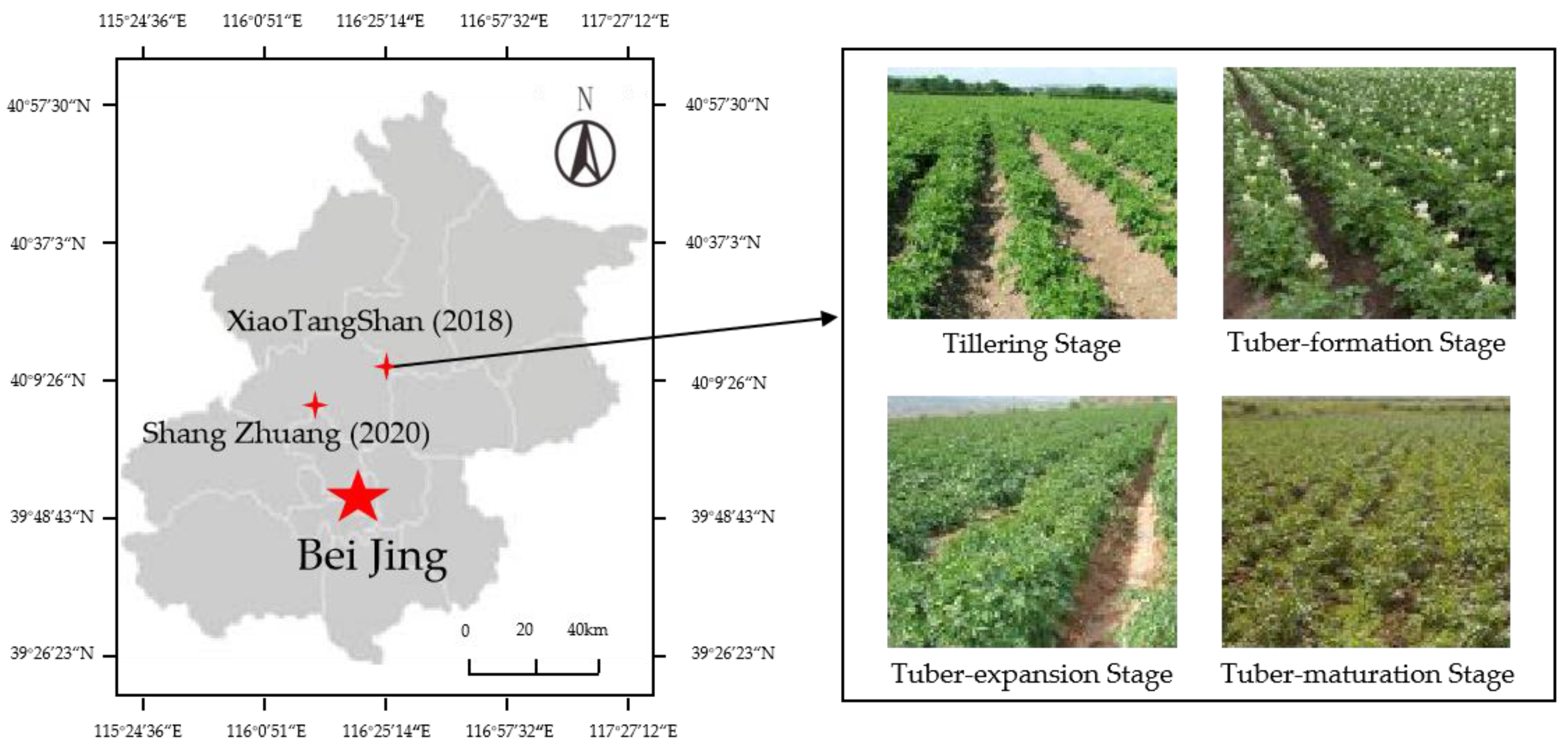
2.1.1. Spectral Data Collection
2.1.2. Chlorophyll Content Measurement
2.2. Data Analysis
2.2.1. SNV Correction
2.2.2. CWT
2.2.3. CARS
2.2.4. PLS Method
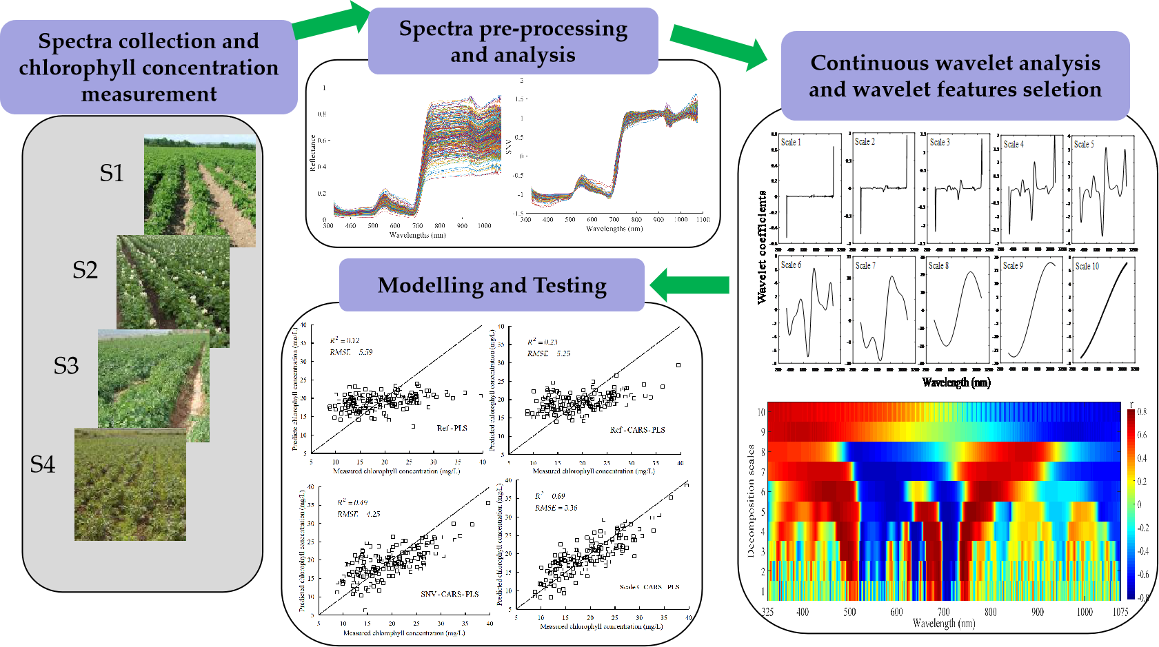
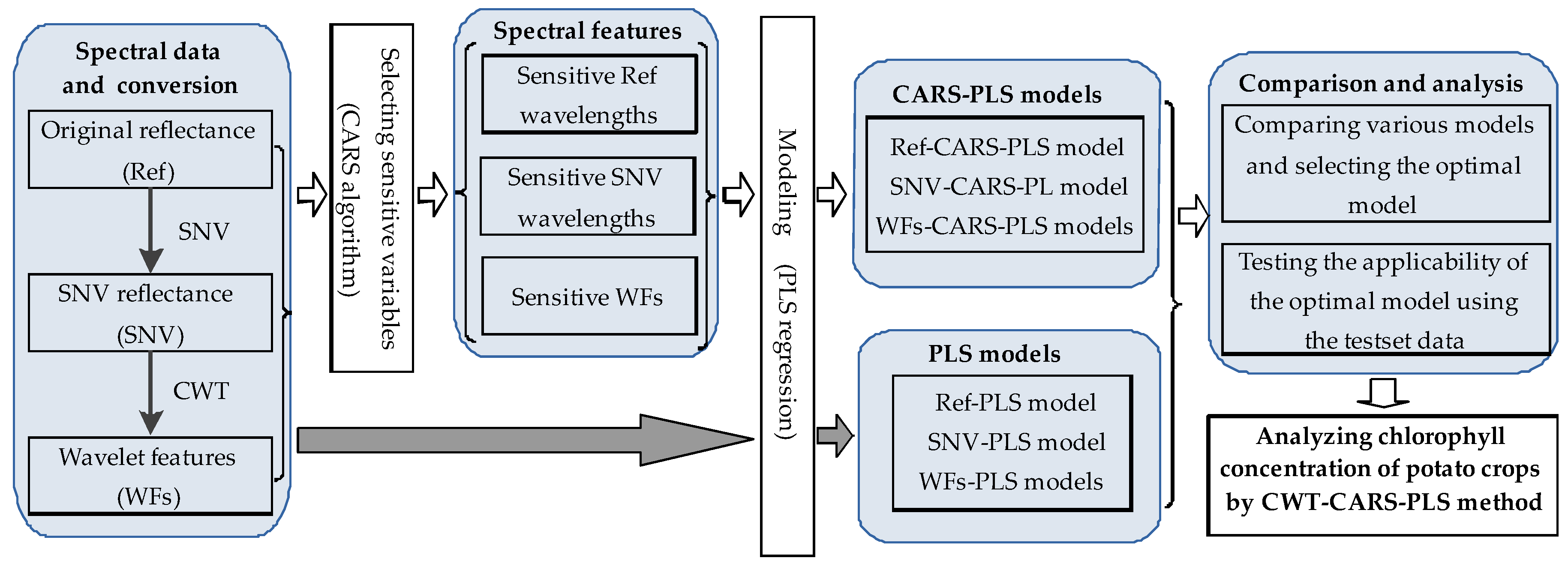
2.2.5. CWT-CARS-PLS
2.3. Model Evaluation Indicators
3. Results
3.1. Statistics on Chlorophyll Concentration of Modeling Data
3.2. Spectral Data Analysis
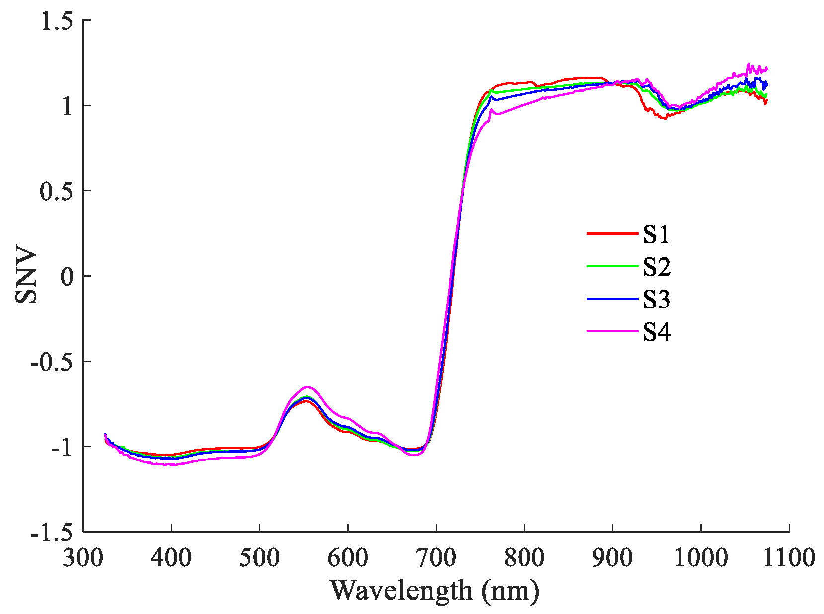
3.2.1. Analysis of Spectral Response during Growth
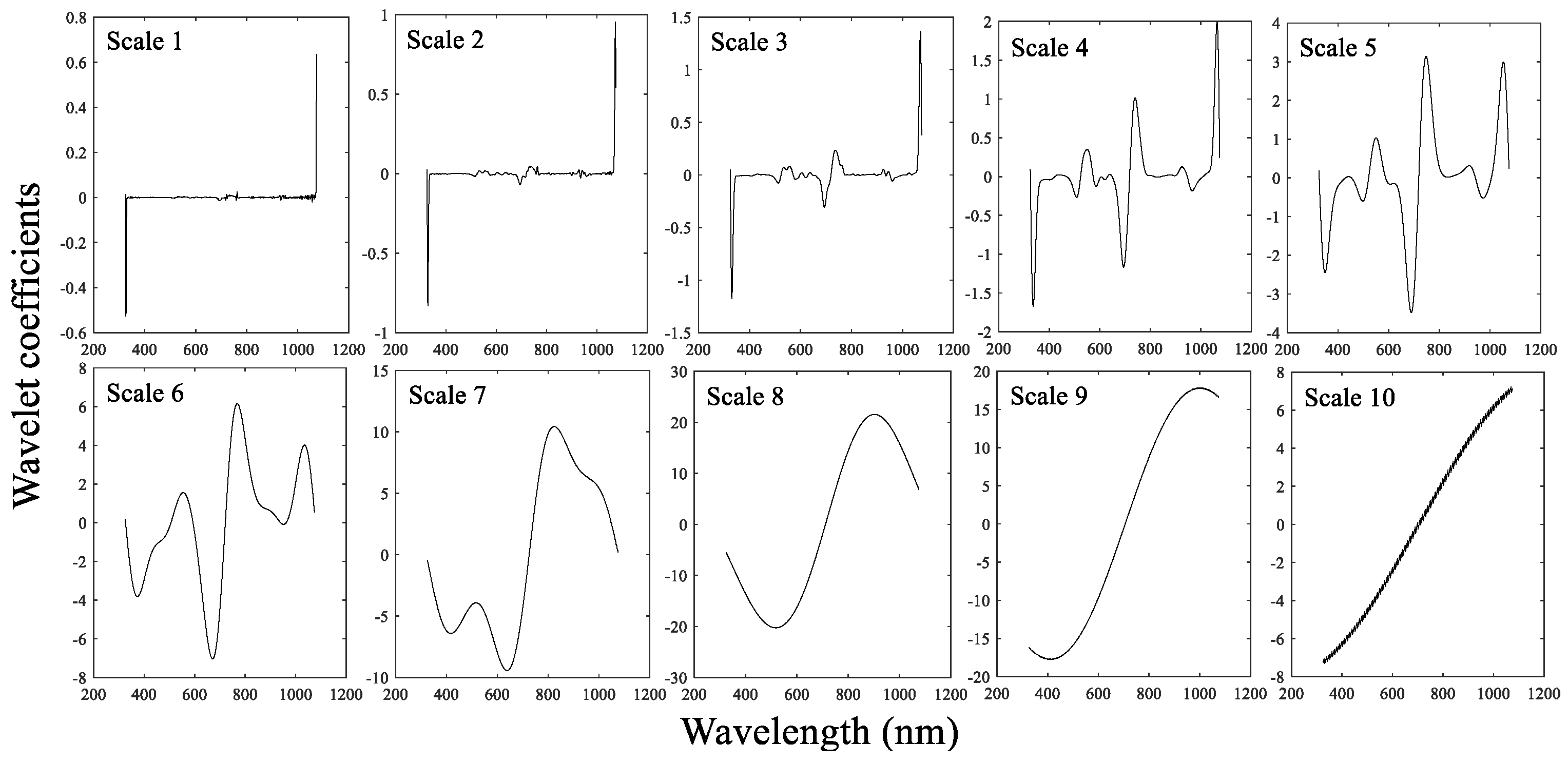
3.2.2. Analysis of Wavelet Coefficient Curves under Different Decomposition Scales
3.3. Correlation of Spectra and Wavelet Features with Chlorophyll Concentration
3.3.1. Correlation Analysis between Chlorophyll Concentration and Spectra
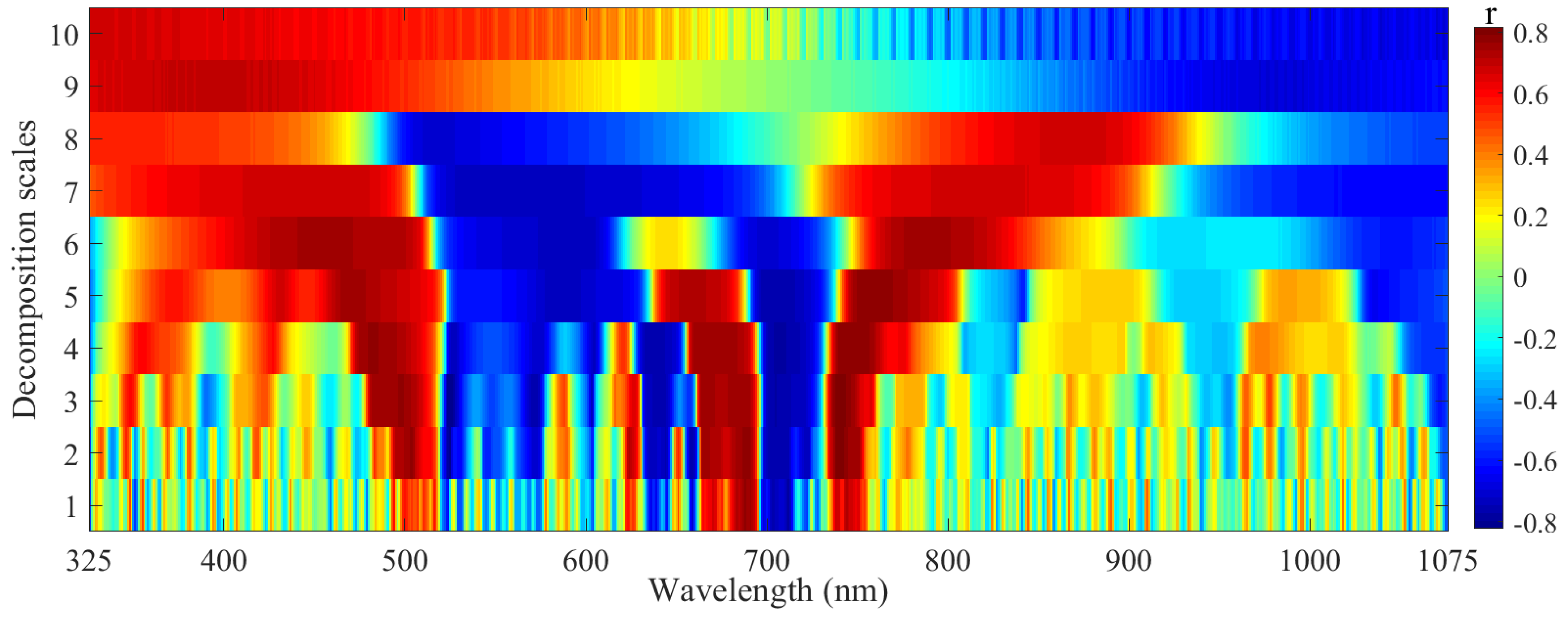
3.3.2. Correlation Analysis between Chlorophyll and Wavelet Features
3.3.3. Comparison of Correlation Coefficient
3.4. Establishment and Comparison of Chlorophyll Analysis Models
3.4.1. Sensitive Chlorophyll Variables Selected Using CARS
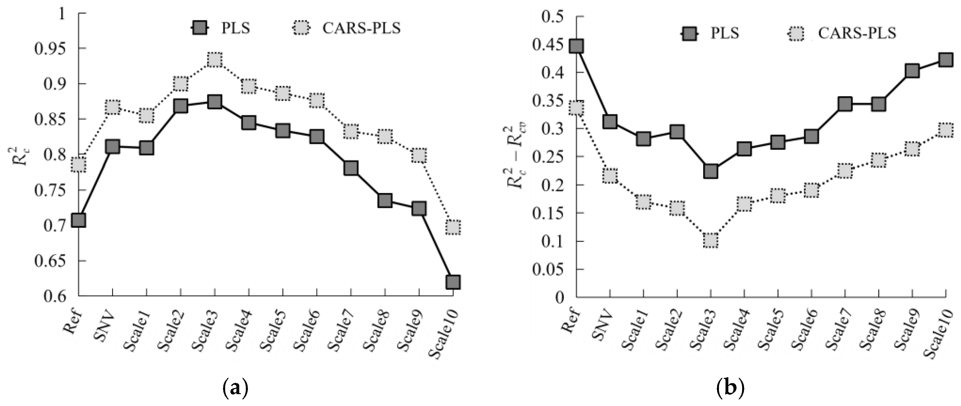
3.4.2. Comparison of the Performance of PLS and CARS-PLS Models
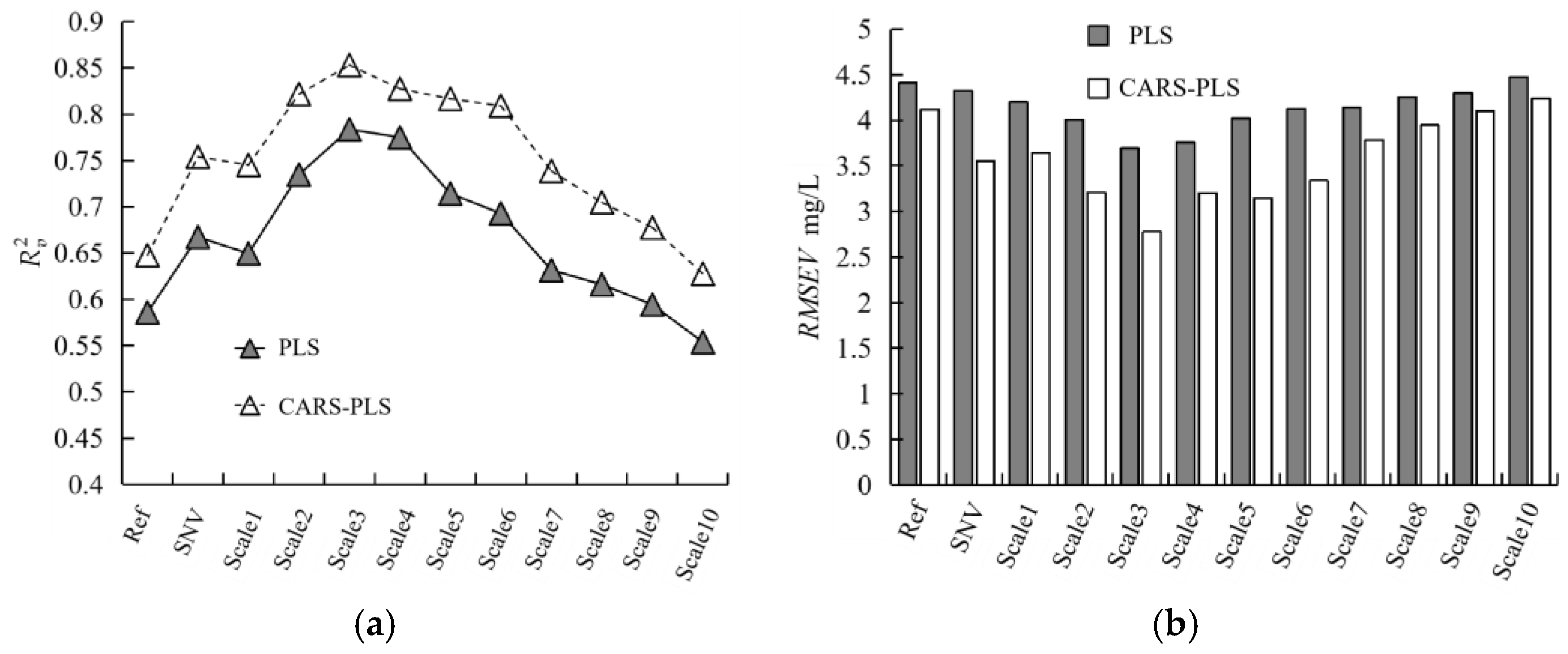
3.5. Validation of Chlorophyll Analysis Models
3.6. Testing of the Developed Scale3-CARS-PLS Model
4. Discussion
4.1. Abilities of Denoising and Sensitive-Variable Mining of CWT at Different Decomposition Scales
4.2. Uninformative Variable Elimination by CARS Algorithm
4.3. Chlorophyll Content Analysis Capability of WFs under Different Decomposition Scales
4.4. Generalizability of This Study to Future Works
5. Conclusions
Author Contributions
Funding
Acknowledgments
Conflicts of Interest
References
- Liu, N.; Zhao, R.; Qiao, L.; Zhang, Y.; Li, M.; Sun, H.; Xing, Z.; Wang, X. Growth stages classification of potato crop based on analysis of spectral response and variables optimization. Sensors 2020, 20, 3995. [Google Scholar] [CrossRef] [PubMed]
- Shillito, R.M.; Timlin, D.J.; Fleisher, D. Yield response of potato to spatially patterned nitrogen application. Agric. Ecosyst. Environ. 2009, 129, 107–116. [Google Scholar] [CrossRef]
- Vesali, F.; Omid, M.; Mobli, H.; Kaleita, A. Feasibility of using smart phones to estimate chlorophyll content in corn plants. Photosynthetica 2017, 55, 603–610. [Google Scholar] [CrossRef]
- Zhenjiang, Z.; Mohamed, J.; Finn, P. Using ground-based spectral reflectance sensors and photography to estimate shoot N concentration and dry matter of potato. Comput. Electron. Agric. 2018, 144, 154–163. [Google Scholar] [CrossRef]
- Clevers, J.G.P.W.; Kooistra, L. Using hyperspectral remote sensing data for retrieving canopy chlorophyll and nitrogen content. In Proceedings of the 2011 3rd Workshop on Hyperspectral Image and Signal Processing: Evolution in Remote Sensing (WHISPERS), Lisbon, Portugal, 6–9 June 2011; pp. 574–583. [Google Scholar] [CrossRef]
- Sonobe, R.; Hirono, Y.; Oi, A. Non-destructive detection of tea leaf chlorophyll content using hyperspectral reflectance and machine learning algorithms. Plants 2020, 99, 368. [Google Scholar] [CrossRef] [PubMed]
- Fairooz, J.; Mat-Jafri, M.Z.; Hwee-San, L.; Wan-Maznah, W.O. Laboratory measurement: Chlorophyll-a concentration measurement with acetone method using spectrophotometer. In Proceedings of the 2014 IEEE International Conference on Industrial Engineering and Engineering Management, Selangor Darul Ehsan, Malaysia, 9–12 December 2015; pp. 744–748. [Google Scholar] [CrossRef]
- Igamberdiev, R.M.; Bill, R.; Schubert, H.; Lennartz, B. Analysis of cross-seasonal spectral response from Kettle Holes: Application of remote sensing techniques for chlorophyll estimation. Remote Sens. 2012, 4, 3481–3500. [Google Scholar] [CrossRef]
- Wen, P.; He, J.; Fang, N. Estimating leaf nitrogen concentration considering unsynchronized maize growth stages with canopy hyperspectral technique. Ecol. Indic. 2019, 107, 1–16. [Google Scholar] [CrossRef]
- Zhang, Y.; Guanter, L.; Berry, J.A.; Christiaan, T.; Yang, X.; Tang, J.; Zhang, F. Model-based analysis of the relationship between sun-induced chlorophyll fluorescence and gross primary production for remote sensing applications. Remote Sens. Environ. 2016, 187, 145–155. [Google Scholar] [CrossRef]
- Thomas, C.A.; Binzel, R.P. Identifying meteorite source regions through near-Earth object spectroscopy. Icarus 2010, 205, 419–429. [Google Scholar] [CrossRef]
- Reddy, V.; Gaffey, M.J.; Abell, P.A.; Hardersen, P.S. Constraining albedo, diameter and composition of near-Earth asteroids via near-infrared spectroscopy. Icarus 2012, 219, 382–392. [Google Scholar] [CrossRef]
- Zhang, J.; Sun, H.; Gao, D.; Qiao, L.; Liu, N.; Li, M.; Zhang, Y. Detection of Canopy Chlorophyll Content of Corn Based on Continuous Wavelet Transform Analysis. Remote Sens. 2020, 12, 2741. [Google Scholar] [CrossRef]
- Nigon, T.J.; Mulla, D.J.; Rosen, C.J. Evaluation of the nitrogen sufficiency index for use with high resolution, broadband aerial imagery in a commercial potato field. Precis. Agric. 2014, 15, 202–226. [Google Scholar] [CrossRef]
- Liu, P.; Sohn, H.; Jeon, I. Nonlinear spectral correlation for fatigue crack detection under noisy environments. J. Sound Vib. 2017, 400, 305–316. [Google Scholar] [CrossRef]
- Silalahi, D.; Midi, H.; Arasan, J.; Mustafa, M.S.; Caliman, J.P. Robust generalized multiplicative scatter correction algorithm on pretreatment of near infrared spectral data. Vib. Spectrosc. 2018, 97, 55–65. [Google Scholar] [CrossRef]
- Zeaiter, M.; Roger, J.M.; Bellon-Maurel, V. Robustness of models developed by multivariate calibration: Part II: The influence of pre-processing methods. TrAC Trends Anal. Chem. 2005, 24, 437–445. [Google Scholar] [CrossRef]
- Fearn, T.; Riccioli, C.; Garrido-Varo, A. On the geometry of SNV and MSC. Chemom. Intell. Lab. Syst. 2009, 96, 22–26. [Google Scholar] [CrossRef]
- Luo, J.; Ying, K.; He, P.; Bai, J. Properties of Savitzky–Golay digital differentiators. Digit. Signal Process. 2005, 15, 122–136. [Google Scholar] [CrossRef]
- Shen, Q.; Zhang, B.; Li, J.; Wu, D.; Song, Y.; Zhang, F.; Wang, G. Characteristic wavelengths analysis for remote sensing reflectance on water surface in Taihu Lake. Spectrosc. Spectr. Anal. 2011, 31, 1892–1897. [Google Scholar] [CrossRef]
- Zhang, Z.; Ding, J.; Zhu, C.; Wang, J. Combination of efficient signal pre-processing and optimal band combination algorithm to predict soil organic matter through visible and near-infrared spectra. Spectrochim. Acta Part. A Mol. Biomol. Spectrosc. 2020, 240, 118553. [Google Scholar] [CrossRef]
- Xu, S.; Wang, M.; Shi, X. Hyperspectral imaging for high-resolution mapping of soil carbon fractions in intact paddy soil profiles with multivariate techniques and variable selection. Geoderma 2020, 370, 114368. [Google Scholar] [CrossRef]
- Rondeaux, G.; Steven, M.; Baret, F. Optimization of soil-adjusted vegetation indices. Remote Sens. Environ. 1996, 55, 95–107. [Google Scholar] [CrossRef]
- Gitelson, A.; Merzlyak, M.N. Spectral reflectance changes associated with autumn senescence of aesculus hippocastanum l. and acer platanoidesl. Leaves. Spectral features and relation to chlorophyll estimation. J. Plant Physiol. 1994, 143, 286–292. [Google Scholar] [CrossRef]
- Salas, E.A.L.; Henebry, G.M. A new approach for the analysis of hyperspectral data: Theory and sensitivity analysis of the moment distance method. Remote Sens 2014, 6, 20–41. [Google Scholar] [CrossRef]
- Sukhova, E.; Sukhov, V. Connection of the photochemical reflectance index (PRI) with the photosystem II quantum yield and nonphotochemical quenching can be dependent on variations of photosynthetic parameters among investigated plants: A meta-analysis. Remote Sens. 2018, 10, 771. [Google Scholar] [CrossRef]
- Yu, K.; Lenz-Wiedemann, V.; Chen, X. Estimating leaf chlorophyll of barley at different growth stages using spectral indices to reduce soil background and canopy structure effects. ISPRS J. Photogramm. Remote Sens. 2014, 97, 58–77. [Google Scholar] [CrossRef]
- Sun, H.; Zheng, T.; Liu, N. Vertical distribution of chlorophyll in potato plants based on hyperspectral imaging. Trans. Chin. Soc. Agric. Eng. 2018, 34, 149–156. [Google Scholar] [CrossRef]
- Sun, J.; Shi, S.; Yang, j.; Gong, W.; Qiu, F.; Wang, L.; Du, L.; Chen, B. Wavelength selection of the multispectral lidar system for estimating leaf chlorophyll and water contents through the PROSPECT model. Agric. For. Meteorol. 2019, 266, 43–52. [Google Scholar] [CrossRef]
- Cheng, T.; Rivard, B.; Sánchez-Azofeifa, A. Spectroscopic determination of leaf water content using continuous wavelet analysis. Remote Sens. Environ. 2011, 115, 659–670. [Google Scholar] [CrossRef]
- Li, D.; Cheng, T.; Zhou, K.; Zheng, H.; Yao, X.; Tian, Y.; Zhu, Y.; Cao, W. WREP: A wavelet-based technique for extracting the red edge position from reflectance spectra for estimating leaf and canopy chlorophyll contents of cereal crops. ISPRS J. Photogramm. Remote Sens. 2017, 129, 103–117. [Google Scholar] [CrossRef]
- Li, D.; Wang, X.; Zheng, H. Estimation of area- and mass-based leaf nitrogen contents of wheat and rice crops from water-removed spectra using continuous wavelet analysis. Plant Methods 2018, 14, 76–96. [Google Scholar] [CrossRef]
- Wang, H.; Huo, Z.; Zhou, G.; Liao, Q.; Feng, H.; Wu, L. Estimating leaf SPAD values of freeze-damaged winter wheat using continuous wavelet analysis. Plant. Physiol. Biochem. 2016, 98, 39–45. [Google Scholar] [CrossRef] [PubMed]
- Lu, J.; Huang, W.; Zhang, J. Quantitative identification of yellow rust and powdery mildew in winter wheat based on wavelet feature. Spectrosc. Spectr. Anal. 2016, 36, 1854–1858. [Google Scholar] [CrossRef]
- Metz, M.; Lesnoff, M.; Abdelghafour, F.; Akbarinia, R.; Masseglia, F.; Roger, J.M. A “big-data” algorithm for KNN-PLS. Chemom. Intell. Lab. Syst. 2020, 104076. [Google Scholar] [CrossRef]
- Huang, Y.; Cao, J.; Ye, S.; Duan, J.; Wu, L.; Li, Q.; Min, S.; Xiong, Y. Near-infrared spectral imaging for quantitative analysis of active component in counterfeit imidacloprid using PLS regression. Optik 2013, 124, 1644–1649. [Google Scholar] [CrossRef]
- Fujiwara, K.; Sawada, H.; Kano, M. Input variable selection for PLS modeling using nearest correlation spectral clustering. Chemom. Intell. Lab. Syst. 2012, 18, 109–119. [Google Scholar] [CrossRef]
- Cai, W.; Li, Y.; Shao, X. A variable selection method based on uninformative variable elimination for multivariate calibration of near-infrared spectra. Chemom. Intell. Lab. 2008, 90, 188–194. [Google Scholar] [CrossRef]
- Mehmood, T.; Liland, K.H.; Snipen, L.; Sæbø, S. A review of variable selection methods in Partial Least Squares Regression. Chemom. Intell. Lab. Syst. 2012, 118, 62–69. [Google Scholar] [CrossRef]
- Li, H.; Xu, Q.; Liang, Y. libPLS: An integrated library for partial least squares regression and linear discriminant analysis. Chemom. Intell. Lab. Syst. 2018, 176, 34–43. [Google Scholar] [CrossRef]
- Devos, O.; Duponchel, L. Parallel genetic algorithm co-optimization of spectral pre-processing and wavelength selection for PLS regression. Chemom. Intell. Lab. Syst. 2011, 107, 50–58. [Google Scholar] [CrossRef]
- Jiang, H.; Zhang, H.; Chen, Q.; Mei, C.; Liu, G. Identification of solid state fermentation degree with FT-NIR spectroscopy: Comparison of wavelength variable selection methods of CARS and SCARS. Spectrochim. Acta Part A Mol. Biomol. Spectrosc. 2015, 149, 1–7. [Google Scholar] [CrossRef]
- Li, H.; Liang, Y.; Xu, Q.; Cao, D. Key wavelengths screening using competitive adaptive reweighted sampling method for multivariate calibration. Anal. Chim. Acta. 2009, 648, 77–84. [Google Scholar] [CrossRef] [PubMed]
- Sumanta, N.; Imranul-Haque, C. Spectrophotometric analysis of chlorophylls and carotenoids from commonly grown fern species by using various extracting solvents. Res. J. Chem. Sci. 2014, 4, 63–69. [Google Scholar] [CrossRef]
- Haitao, S.; Peiqiang, Y. Comparison of grating-based near-infrared (NIR) and Fourier transform mid-infrared (ATR-FT/MIR) spectroscopy based on spectral preprocessing and wavelength selection for the determination of crude protein and moisture content in wheat. Food Control 2017, 82, 57–65. [Google Scholar] [CrossRef]
- Barnes, R.J.; Dhanoa, M.S.; Lister, S.J. Standard normal variate transformation and de-trending of near-infrared diffuse reflectance spectra. Appl. Spectrosc. 1989, 43, 772–777. [Google Scholar] [CrossRef]
- Miller, J.R.; Hare, E.W.; Wu, J. Quantitative characterization of the vegetation red edge reflectance 1. An inverted-Gaussian reflectance model. Int. J. Remote Sens. 1990, 11, 1755–1773. [Google Scholar] [CrossRef]
- Maire, G.; François, C.; Dufrêne, E. Towards universal broad leaf chlorophyll indices using PROSPECT simulated database and hyperspectral reflectance measurements. Remote Sens. Environ. 2004, 89, 1–28. [Google Scholar] [CrossRef]
- Zheng, K.; Li, Q.; Wang, J.; Geng, J.; Cao, P.; Sui, T.; Wang, X.; Du, Y. Stability competitive adaptive reweighted sampling (SCARS) and its applications to multivariate calibration of NIR spectra. Chemom. Intell. Lab. Syst. 2012, 112, 48–54. [Google Scholar] [CrossRef]
- Li, Q.; Huang, Y.; Song, X.; Zhang, J.; Min, S. Moving window smoothing on the ensemble of competitive adaptive reweighted sampling algorithm. Spectrochim. Acta Part A Mol. Biomol. Spectrosc. 2019, 214, 129–138. [Google Scholar] [CrossRef] [PubMed]
- Geladi, P.; Kowalski, B.R. Partial least-squares regression: A tutorial. Anal. Chim. Acta 1986, 185, 1–17. [Google Scholar] [CrossRef]
- Wang, Z.; Sakuno, Y.; Koike, K. Evaluation of chlorophyll-a estimation approaches using iterative stepwise elimination partial least squares (ISE-PLS) regression and several traditional algorithms from field hyperspectral measurements in the Seto Inland Sea, Japan. Sensors 2018, 18, 2656. [Google Scholar] [CrossRef]
- Galvão, R.K.; Araujo, M.C.; José, G.E. A method for calibration and validation subset partitioning. Talanta 2005, 67, 736–740. [Google Scholar] [CrossRef] [PubMed]
- Tian, H.; Zhang, L.; Li, M. Weighted SPXY method for calibration set selection for composition analysis based on near-infrared spectroscopy. Infrared Phys. Technol. 2018, 95, 88–92. [Google Scholar] [CrossRef]
- Meroni, M.; Rossini, M.; Guanter, L.; Alonso, L.; Rascher, U.; Colombo, R.; Moreno, J. Remote sensing of solar-induced chlorophyll fluorescence: Review of methods and applications. Remote Sens. Environ. 2009, 113, 2037–2051. [Google Scholar] [CrossRef]
- Singhal, G.; Bansod, B.; Mathew, L.; Goswami, J.; Choudhury, B.U.; Raju, P.L.N. Chlorophyll estimation using multi-spectral unmanned aerial system based on machine learning techniques. Remote Sens. Appl. Soc. Environ. 2019, 15, 100235. [Google Scholar] [CrossRef]
- Awgchew, H.; Gebremedhi, H.; Taddesse, G. Influence of nitrogen rate on nitrogen use efficiency and quality of potato (Solanum tuberosum L.) varieties at Debre Berhan, Central Highlands of Ethiopia. Int. J. Soil Sci. 2016, 12, 10–17. [Google Scholar] [CrossRef]
- Guo, Y.; Zhou, Y.; Tan, J. Wavelet analysis of pulse-amplitude-modulated chlorophyll fluorescence for differentiation of plant samples. J. Theor. Biol. 2015, 370, 116–120. [Google Scholar] [CrossRef]
- Wang, Z.; Chen, J.; Fan, Y. Evaluating photosynthetic pigment contents of maize using UVE-PLS based on continuous wavelet transform. Comput. Electron. Agric. 2020, 169, 105–160. [Google Scholar] [CrossRef]
- Li, D.; Cheng, T.; Jia, M. PROCWT: Coupling PROSPECT with continuous wavelet transform to improve the retrieval of foliar chemistry from leaf bidirectional reflectance spectra. Remote Sens. Environ. 2018, 206, 1–14. [Google Scholar] [CrossRef]
- Li, Y.; Brian, K.V.; Li, Y. Lifting wavelet transform for Vis-NIR spectral data optimization to predict wood density. Spectrochim. Acta Part A Mol. Biomol. Spectrosc. 2020, 118566. [Google Scholar] [CrossRef]
- Huang, X.; Luo, Y.; Xia, L. An efficient wavelength selection method based on the maximal information coefficient for multivariate spectral calibration. Chemom. Intell. Lab. Syst. 2019, 194, 103872. [Google Scholar] [CrossRef]
- Sun, H.; Liu, N.; Wu, L.; Chen, L.; Yang, L.; Li, M.; Zhang, Q. Water content detection of potato leaves based on hyperspectral image. IFAC PapersOnLine 2018, 51, 443–448. [Google Scholar] [CrossRef]
- Li, H.; Liang, Y.; Xu, Q.; Cao, D. Model population analysis for variable selection. J. Chemom. 2009, 24, 418–423. [Google Scholar] [CrossRef]
- Andries, J.P.M.; Vander Heyden, Y.; Buydens, L.M.C. Improved variable reduction in partial least squares modelling based on Predictive-Property-Ranked Variables and adaptation of partial least squares complexity. Anal. Chim. Acta 2011, 705, 292–305. [Google Scholar] [CrossRef]
- Gourvénec, S.; Fernández-Pierna, J.A.; Massart, D.L.; Rutledge, D.N. An evaluation of the PoLiSh smoothed regression and the Monte Carlo Cross-Validation for the determination of the complexity of a PLS model. Chemom. Intell. Lab. Syst. 2003, 68, 41–51. [Google Scholar] [CrossRef]
- Qiao, L.; Zhang, Z.; Chen, L.; Sun, H.; Li, M.; Li, L.; Ma, J. Detection of chlorophyll content in Maize Canopy from UAV Imagery. IFAC PapersOnLine 2019, 52, 330–335. [Google Scholar] [CrossRef]
- Li, L.; Ren, T.; Ma, Y.; Wei, Q.; Wang, S.; Li, X.; Cong, R.; Liu, S.; Lu, J. Evaluating chlorophyll density in winter oilseed rape (Brassica napus L.) using canopy hyperspectral red-edge parameters. Comput. Electron. Agric. 2016, 126, 21–31. [Google Scholar] [CrossRef]
- Tao, Z.; Ning, L.; Li, W.; Li, M.; Sun, H.; Zhang, Q.; Wu, J. Estimation of Chlorophyll Content in Potato Leaves Based on Spectral Red Edge Position. IFAC PapersOnLine 2018, 51, 602–606. [Google Scholar] [CrossRef]
- Ji, R.; Shi, W.; Wang, Y.; Zhang, H.; Min, J. Nondestructive estimation of bok choy nitrogen status with an active canopy sensor in comparison to a chlorophyll meter. Pedosphere 2020, 30, 769–777. [Google Scholar] [CrossRef]
- Liu, N.; Liu, G.; Sun, H. Real-time detection on spad value of potato plant using an in-field spectral imaging sensor system. Sensors 2020, 20, 3430. [Google Scholar] [CrossRef]


| Growth Stage | Potato-Crop Characteristics | Samples | |
|---|---|---|---|
| Modelling | Testing | ||
| S1 | Appearing flower buds, having about 12 leaves | 74 | 40 |
| S2 | Appearing flowers | 80 | 40 |
| S3 | Flowers falling, stems and leaves aging | 80 | 40 |
| S4 | Stems and leaves withering, upper leaves turning yellow | 80 | 40 |
| Samples | Data Set | Sample Number | Max (mg/L) | Min (mg/L) | Mean (mg/L) | STD (mg/L) |
|---|---|---|---|---|---|---|
| S1 | All | 74 | 40.77 | 17.64 | 28.12 | 5.05 |
| Calibration | 50 | 40.77 | 17.64 | 28.27 | 5.31 | |
| Validation | 24 | 33.12 | 19.64 | 27.48 | 3.86 | |
| S2 | All | 80 | 41.20 | 16.30 | 31.04 | 5.81 |
| Calibration | 50 | 41.20 | 16.30 | 30.23 | 6.29 | |
| Validation | 30 | 37.46 | 25.26 | 33.45 | 3.04 | |
| S3 | All | 80 | 35.63 | 13.70 | 22.00 | 4.18 |
| Calibration | 50 | 35.63 | 13.70 | 22.04 | 4.65 | |
| Validation | 30 | 26.47 | 16.39 | 21.86 | 2.36 | |
| S4 | All | 80 | 32.25 | 7.66 | 15.36 | 5.45 |
| Calibration | 50 | 32.25 | 7.66 | 15.73 | 5.93 | |
| Validation | 30 | 20.69 | 8.20 | 14.24 | 3.55 | |
| All stages | All | 314 | 41.20 | 7.66 | 24.05 | 7.95 |
| Calibration | 200 | 41.20 | 7.66 | 24.07 | 7.95 | |
| Validation | 114 | 37.46 | 8.20 | 24.00 | 8.00 |
| Feature Location | Highest r | |
|---|---|---|
| Wavelength (nm) | ||
| Ref | 698 | −0.50 |
| SNV | 761 | 0.75 |
| Scale 1 | 687 | −0.78 |
| Scale 2 | 739 | 0.81 |
| Scale 3 | 524 | −0.82 |
| Scale 4 | 744 | 0.78 |
| Scale 5 | 755 | 0.79 |
| Scale 6 | 786 | 0.75 |
| Scale 7 | 547 | −0.74 |
| Scale 8 | 515 | −0.71 |
| Scale 9 | 400 | 0.70 |
| Scale 10 | 1038 | −0.70 |
| Models | Variables Number | PCs | Models | Variables Number | PCs |
|---|---|---|---|---|---|
| Ref-CARS-PLS | 61 | 21 | Scale 5-CARS-PLS | 227 | 21 |
| SNV-CARS-PLS | 64 | 17 | Scale 6-CARS-PLS | 48 | 17 |
| Scale 1-CARS-PLS | 31 | 12 | Scale 7-CARS-PLS | 33 | 15 |
| Scale 2-CARS-PLS | 61 | 13 | Scale 8-CARS-PLS | 54 | 18 |
| Scale 3-CARS-PLS | 57 | 3 | Scale 9-CARS-PLS | 57 | 17 |
| Scale 4-CARS-PLS | 178 | 19 | Scale 10-CARS-PLS | 33 | 28 |
© 2020 by the authors. Licensee MDPI, Basel, Switzerland. This article is an open access article distributed under the terms and conditions of the Creative Commons Attribution (CC BY) license (http://creativecommons.org/licenses/by/4.0/).
Share and Cite
Liu, N.; Xing, Z.; Zhao, R.; Qiao, L.; Li, M.; Liu, G.; Sun, H. Analysis of Chlorophyll Concentration in Potato Crop by Coupling Continuous Wavelet Transform and Spectral Variable Optimization. Remote Sens. 2020, 12, 2826. https://doi.org/10.3390/rs12172826
Liu N, Xing Z, Zhao R, Qiao L, Li M, Liu G, Sun H. Analysis of Chlorophyll Concentration in Potato Crop by Coupling Continuous Wavelet Transform and Spectral Variable Optimization. Remote Sensing. 2020; 12(17):2826. https://doi.org/10.3390/rs12172826
Chicago/Turabian StyleLiu, Ning, Zizheng Xing, Ruomei Zhao, Lang Qiao, Minzan Li, Gang Liu, and Hong Sun. 2020. "Analysis of Chlorophyll Concentration in Potato Crop by Coupling Continuous Wavelet Transform and Spectral Variable Optimization" Remote Sensing 12, no. 17: 2826. https://doi.org/10.3390/rs12172826
APA StyleLiu, N., Xing, Z., Zhao, R., Qiao, L., Li, M., Liu, G., & Sun, H. (2020). Analysis of Chlorophyll Concentration in Potato Crop by Coupling Continuous Wavelet Transform and Spectral Variable Optimization. Remote Sensing, 12(17), 2826. https://doi.org/10.3390/rs12172826