Evaluating the Effects of Digital Elevation Models in Landslide Susceptibility Mapping in Rangamati District, Bangladesh


Abstract

1. Introduction
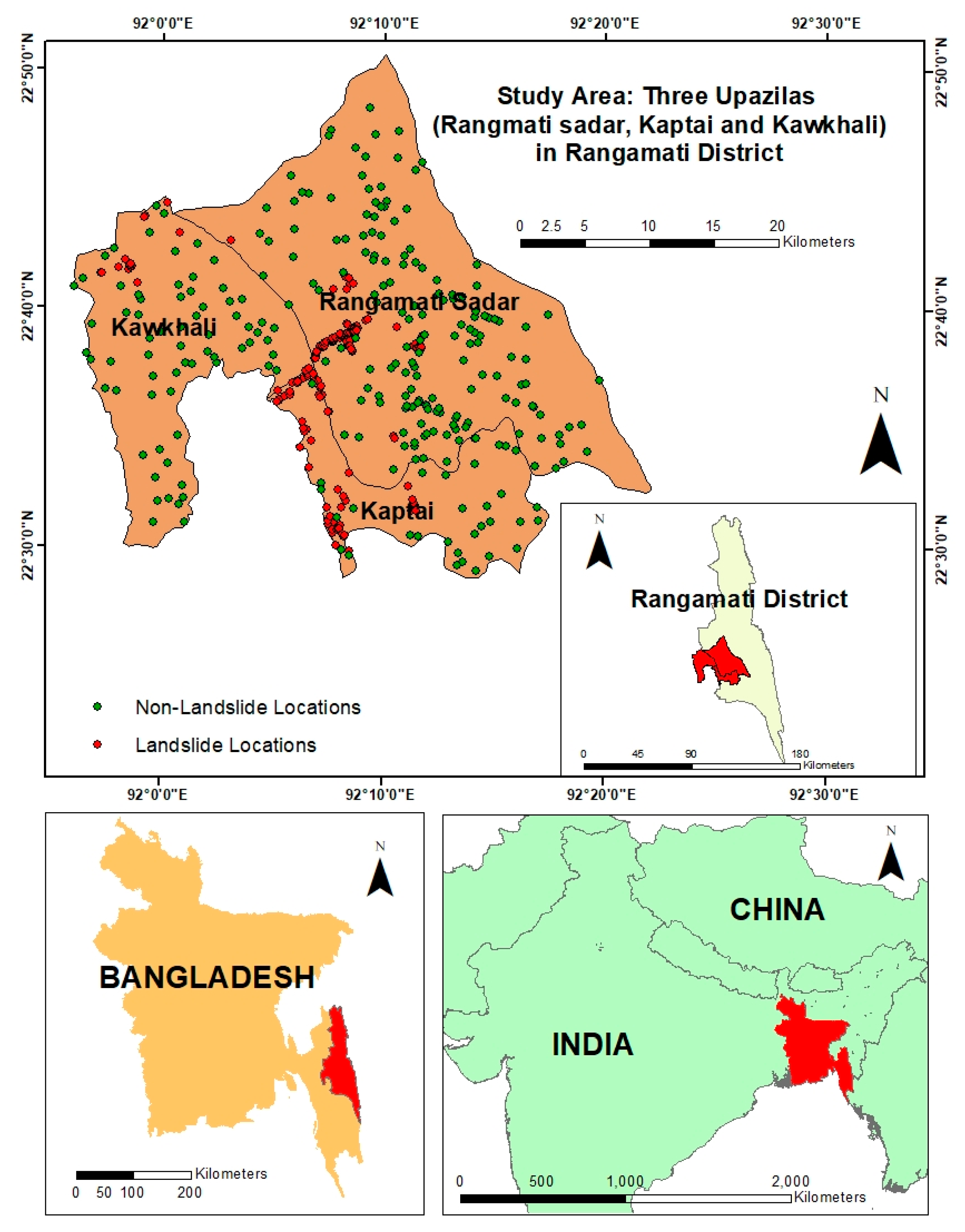
2. Study Area
3. Synopsis on Data Utilization
3.1. Landslide Inventory
3.2. Landslide Causal Factors
3.2.1. Elevation
3.2.2. Slope
3.2.3. Aspect
3.2.4. Plan Curvature and Profile Curvature
3.2.5. Topographic Wetness Index and Stream Power Index
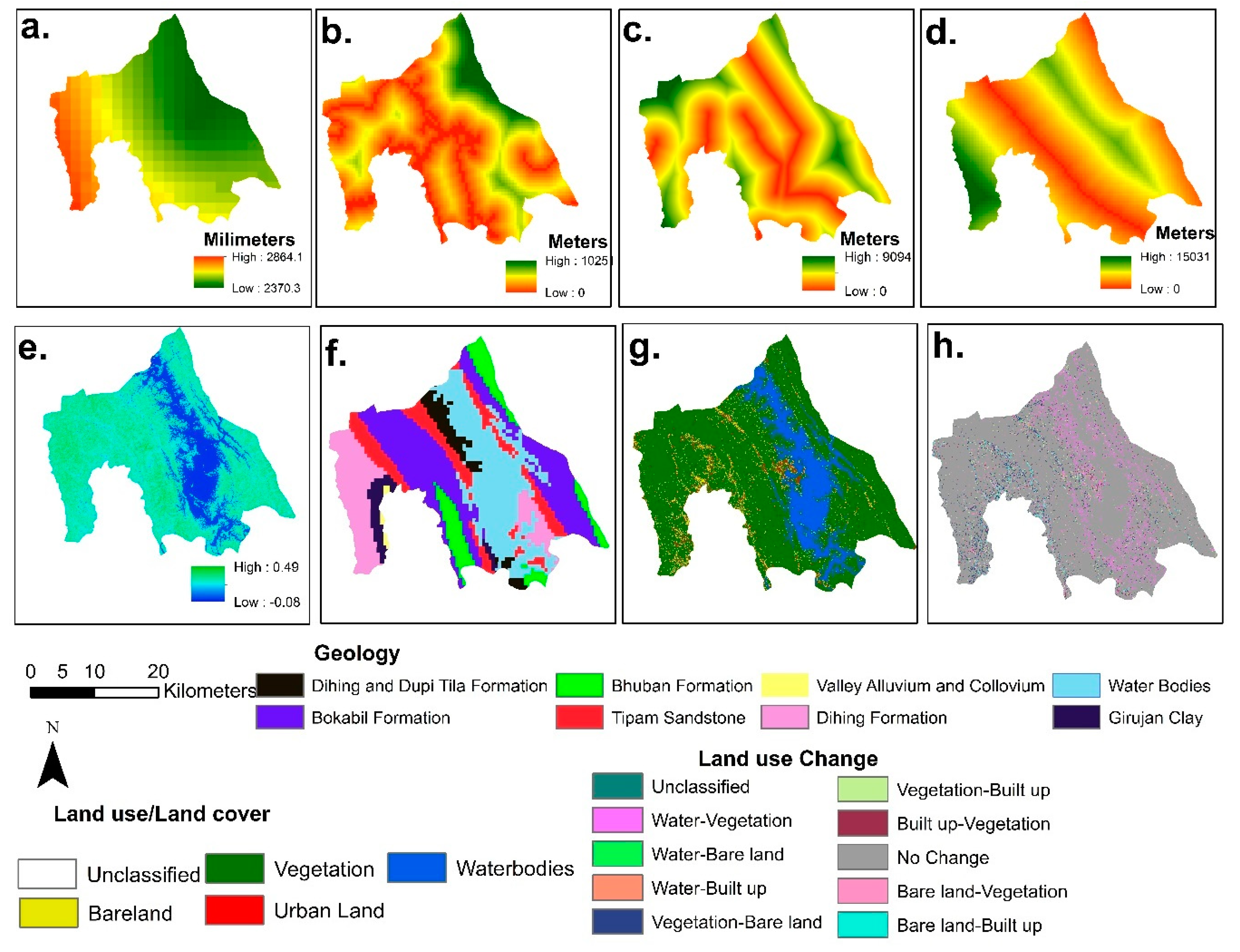
3.3. Rainfall
3.4. Distance-Based Causal Factors
3.5. Normalized Difference Vegetation Index (NDVI)
3.6. Geology
3.7. Land Use land Cover
4. Methodology
4.1. Training and Validation Dataset
4.2. Modified Frequency Ratio (MFR)
4.3. Logistic Regression (LR)
4.4. Random Forest Classification (RF)
4.5. Multicollinearity Diagnostics
4.6. Model Validation and Comparison
5. Results
5.1. Susceptibility Assessment Using Modified Frequency Ratio (MFR)
Landslide Susceptibility Maps (MFR)
5.2. Susceptibility Assessment using Logistic Regression (LR)
Landslide Susceptibility Maps (LR)
5.3. Susceptibility Assessment using Random Forest (RF)
Landslide Susceptibility Maps (RF)
5.4. Validation and Comparison of Landslide Susceptibility Maps
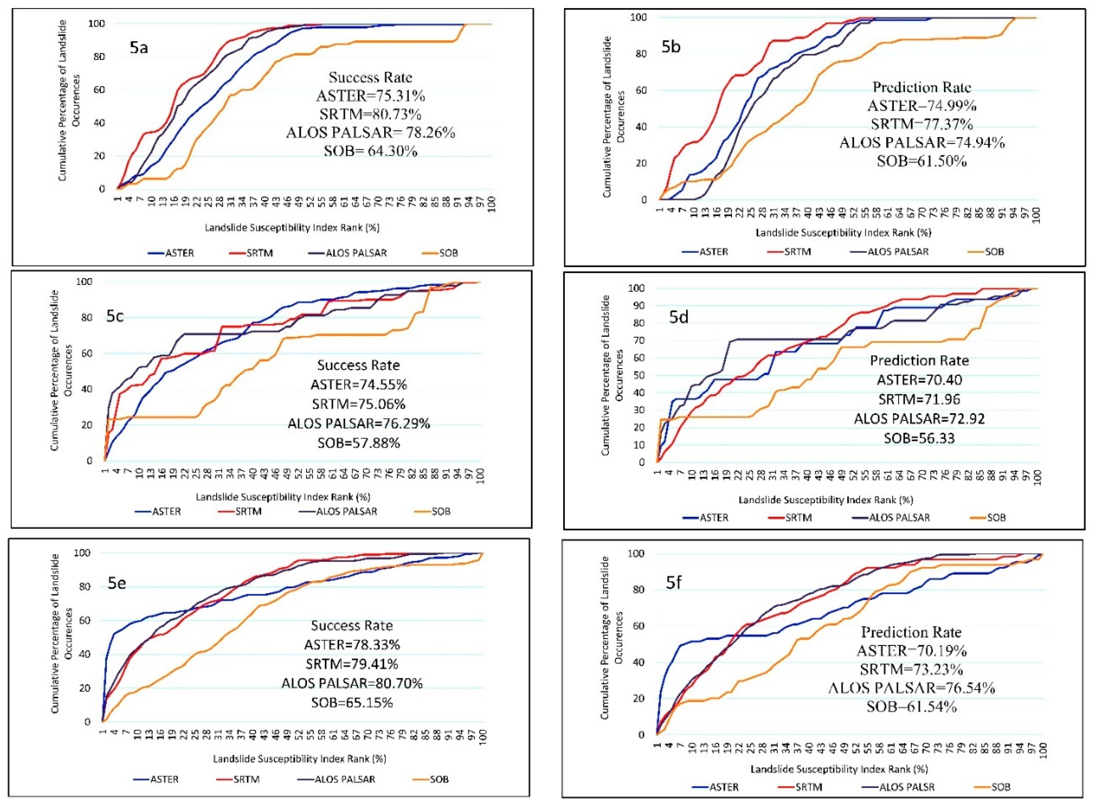
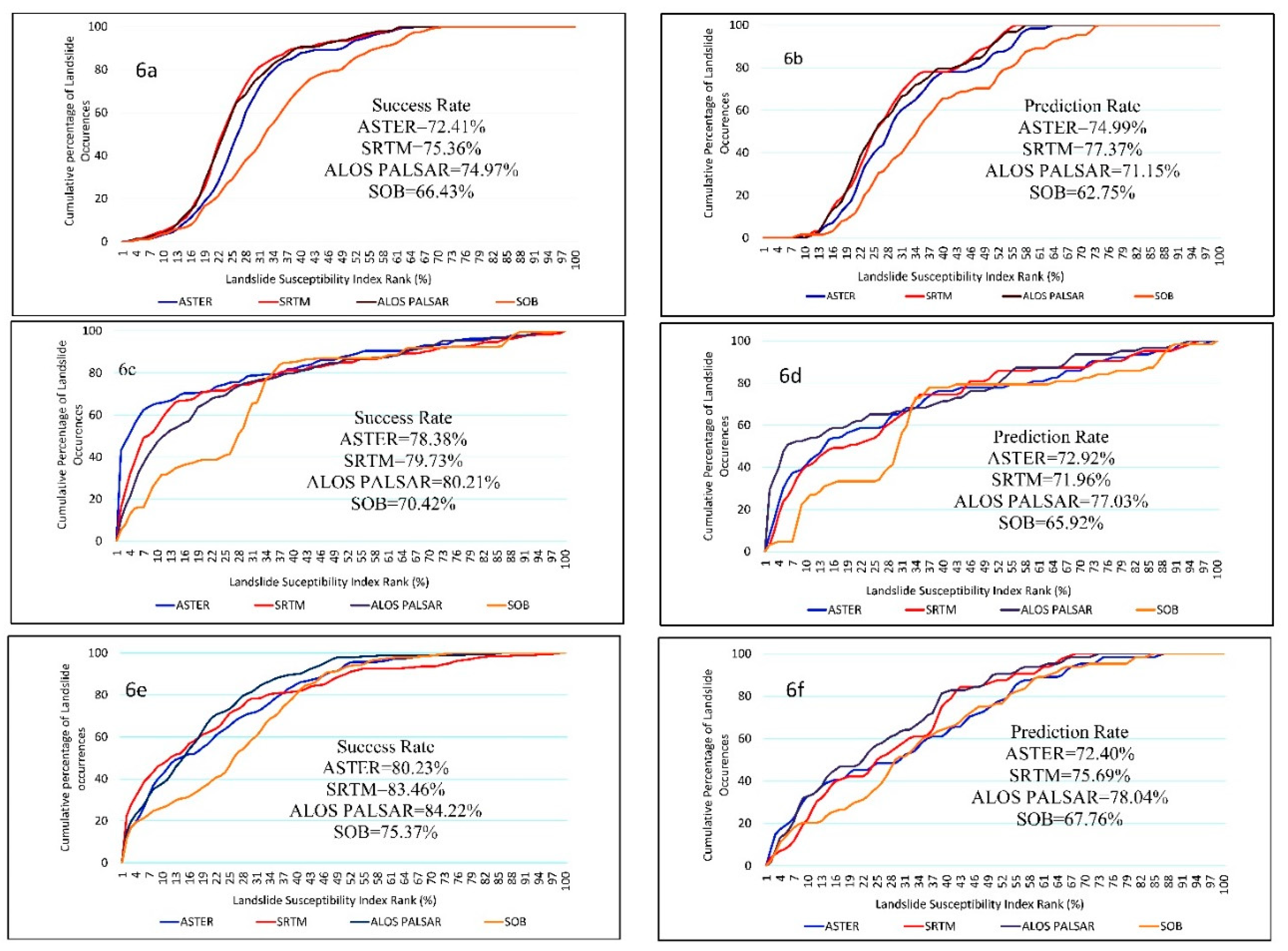
5.4.1. Success and Prediction Rate Curves
DEM-Based Causal Factors
All Causal Factors
5.4.2. Spatial Comparison of Landslide Susceptibility Maps
6. Discussion
7. Conclusions
Author Contributions
Funding
Acknowledgments
Conflicts of Interest
Appendix A

Appendix B

Appendix C

Appendix D

| Causal Factors | Classes | Area (%), | Landslides (%), | FR, | RF, | MinRF | MaxRF | (MaxRF - MinRF) | PR |
|---|---|---|---|---|---|---|---|---|---|
| Aspect (ASTER) | Flat | 0.00 | 0.00 | 0.00 | 0.00 | 0.03 | 0.17 | 0.14 | 1.00 |
| North | 16.7 | 4.17 | 0.25 | 0.03 | |||||
| Northeast | 11.5 | 11.46 | 1.00 | 0.11 | |||||
| East | 11.3 | 17.71 | 1.57 | 0.17 | |||||
| Southeast | 10.2 | 13.54 | 1.33 | 0.14 | |||||
| South | 10.4 | 13.02 | 1.25 | 0.13 | |||||
| Southwest | 13.1 | 18.23 | 1.39 | 0.15 | |||||
| West | 12.1 | 7.81 | 0.65 | 0.07 | |||||
| Northwest | 10.1 | 9.90 | 0.98 | 0.11 | |||||
| North | 4.6 | 4.17 | 0.91 | 0.10 | |||||
| Aspect (SRTM) | Flat | 0.00 | 0.00 | 0.00 | 0.00 | 0.03 | 0.16 | 0.13 | 1.00 |
| North | 17.40 | 4.69 | 0.27 | 0.03 | |||||
| Northeast | 10.99 | 10.42 | 0.95 | 0.10 | |||||
| East | 11.19 | 16.67 | 1.49 | 0.16 | |||||
| Southeast | 10.31 | 10.94 | 1.06 | 0.11 | |||||
| South | 10.45 | 13.02 | 1.25 | 0.13 | |||||
| Southwest | 13.45 | 20.31 | 1.51 | 0.16 | |||||
| West | 12.31 | 11.98 | 0.97 | 0.10 | |||||
| Northwest | 9.65 | 7.81 | 0.81 | 0.09 | |||||
| North | 4.26 | 4.17 | 0.98 | 0.11 | |||||
| Aspect (ALOS PALSAR) | Flat | 0.00 | 0.00 | 0.00 | 0.00 | 0.03 | 0.17 | 0.14 | 1.00 |
| North | 17.81 | 4.69 | 0.26 | 0.03 | |||||
| Northeast | 10.98 | 10.42 | 0.95 | 0.10 | |||||
| East | 10.71 | 16.67 | 1.56 | 0.17 | |||||
| Southeast | 10.71 | 10.94 | 1.02 | 0.11 | |||||
| South | 10.35 | 13.02 | 1.26 | 0.13 | |||||
| Southwest | 13.39 | 20.31 | 1.52 | 0.16 | |||||
| West | 11.84 | 11.98 | 1.01 | 0.11 | |||||
| Northwest | 9.92 | 7.81 | 0.79 | 0.08 | |||||
| North | 4.29 | 4.17 | 0.97 | 0.10 | |||||
| Aspect (SOB) | Flat | 22.99 | 13.76 | 0.60 | 0.05 | 0.03 | 0.40 | 0.37 | 2.37 |
| North | 8.59 | 3.17 | 0.37 | 0.03 | |||||
| Northeast | 8.73 | 5.29 | 0.61 | 0.05 | |||||
| East | 7.25 | 3.17 | 0.44 | 0.04 | |||||
| Southeast | 6.14 | 29.10 | 4.74 | 0.40 | |||||
| South | 7.73 | 6.35 | 0.82 | 0.07 | |||||
| Southwest | 12.35 | 11.11 | 0.90 | 0.08 | |||||
| West | 12.03 | 11.11 | 0.92 | 0.08 | |||||
| Northwest | 8.10 | 10.58 | 1.31 | 0.11 | |||||
| North | 6.08 | 6.35 | 1.04 | 0.09 | |||||
| Elevation (m) (ASTER) | <47 | 43.64 | 22.92 | 0.53 | 0.11 | 0.00 | 0.50 | 0.50 | 3.57 |
| 47–89 | 33.46 | 40.10 | 1.20 | 0.26 | |||||
| 89–156 | 14.33 | 33.33 | 2.33 | 0.50 | |||||
| 156–264 | 6.52 | 3.65 | 0.56 | 0.12 | |||||
| 264–577 | 2.06 | 0.00 | 0.00 | 0.00 | |||||
| Elevation (m) (SRTM) | <60 | 52.93 | 26.56 | 0.50 | 0.11 | 0.00 | 0.41 | 0.41 | 3.05 |
| 60–108 | 30.88 | 53.65 | 1.74 | 0.38 | |||||
| 108–178 | 9.16 | 17.19 | 1.88 | 0.41 | |||||
| 178–282 | 5.29 | 2.60 | 0.49 | 0.11 | |||||
| 282–577 | 1.75 | 0.00 | 0.00 | 0.00 | |||||
| Elevation (m) (ALOS PALSAR) | <5 | 51.07 | 26.04 | 0.51 | 0.11 | 0.00 | 0.44 | 0.44 | 3.15 |
| 5–54 | 32.46 | 52.08 | 1.60 | 0.35 | |||||
| 54–126 | 9.52 | 19.27 | 2.03 | 0.44 | |||||
| 126–229 | 5.22 | 2.60 | 0.50 | 0.11 | |||||
| 229–526 | 1.74 | 0.00 | 0.00 | 0.00 | |||||
| Elevation (m) (SOB) | <56 | 52.90 | 32.11 | 0.61 | 0.14 | 0.05 | 0.43 | 0.38 | 2.41 |
| 56–111 | 24.38 | 45.79 | 1.88 | 0.43 | |||||
| 111–174 | 13.96 | 20.00 | 1.43 | 0.33 | |||||
| 174–248 | 4.91 | 1.05 | 0.21 | 0.05 | |||||
| 248–498 | 3.86 | 1.05 | 0.27 | 0.06 | |||||
| Slope (º) (ASTER) | <4 | 33.20 | 12.50 | 0.38 | 0.06 | 0.06 | 0.31 | 0.31 | 2.22 |
| 4–8 | 28.17 | 23.96 | 0.85 | 0.13 | |||||
| 8–14 | 21.88 | 30.73 | 1.40 | 0.22 | |||||
| 14–22 | 12.64 | 25.52 | 2.02 | 0.31 | |||||
| 22–52 | 4.10 | 7.29 | 1.78 | 0.28 | |||||
| Slope (º) (SRTM) | <3 | 32.81 | 8.85 | 0.27 | 0.04 | 0.04 | 0.33 | 0.28 | 2.12 |
| 3–8 | 30.18 | 26.56 | 0.88 | 0.15 | |||||
| 8–14 | 21.92 | 37.50 | 1.71 | 0.28 | |||||
| 14–22 | 11.59 | 22.92 | 1.98 | 0.33 | |||||
| 22–61 | 3.51 | 4.17 | 1.19 | 0.20 | |||||
| Slope (º) (ALOS PALSAR) | <4 | 32.64 | 5.73 | 0.18 | 0.03 | 0.03 | 0.34 | 0.31 | 2.25 |
| 4–9 | 28.63 | 27.60 | 0.96 | 0.16 | |||||
| 9–15 | 22.79 | 36.46 | 1.60 | 0.26 | |||||
| 15–23 | 12.29 | 25.52 | 2.08 | 0.34 | |||||
| 23–65 | 3.65 | 4.69 | 1.28 | 0.21 | |||||
| Slope (º) (SOB) | <2 | 60.16 | 48.68 | 1.50 | 0.45 | 0.07 | 0.35 | 0.28 | 1.79 |
| 2–4 | 22.75 | 28.04 | 0.81 | 0.16 | |||||
| 4–8 | 11.49 | 20.63 | 1.23 | 0.24 | |||||
| 8–14 | 4.50 | 1.59 | 1.80 | 0.35 | |||||
| 14–46 | 1.10 | 1.06 | 0.35 | 0.07 | |||||
| TWI (ASTER) | <6 | 40.58 | 60.94 | 1.50 | 0.45 | 0.00 | 0.45 | 0.45 | 3.19 |
| 6–8 | 29.20 | 29.17 | 1.00 | 0.30 | |||||
| 8–11 | 12.33 | 6.77 | 0.55 | 0.16 | |||||
| 11–14 | 10.90 | 3.12 | 0.29 | 0.09 | |||||
| >14 | 6.98 | 0.00 | 0.00 | 0.00 | |||||
| TWI (SRTM) | <6 | 45.22 | 71.35 | 1.58 | 0.54 | 0.00 | 0.54 | 0.54 | 4.03 |
| 6–8 | 26.17 | 23.96 | 0.92 | 0.31 | |||||
| 8–11 | 10.29 | 3.65 | 0.35 | 0.12 | |||||
| 11–14 | 12.04 | 1.04 | 0.09 | 0.03 | |||||
| >14 | 6.28 | 0.00 | 0.00 | 0.00 | |||||
| TWI (ALOS PALSAR) | <6 | 44.46 | 76.04 | 1.71 | 0.60 | 0.00 | 0.60 | 0.60 | 4.30 |
| 6–9 | 29.03 | 18.23 | 0.63 | 0.22 | |||||
| 9–12 | 9.11 | 3.65 | 0.40 | 0.14 | |||||
| 12–15 | 15.41 | 2.08 | 0.14 | 0.05 | |||||
| >15 | 1.99 | 0.00 | 0.00 | 0.00 | |||||
| TWI (SOB) | <8 | 24.42 | 29.63 | 1.21 | 0.29 | 0.04 | 0.29 | 0.25 | 1.61 |
| 8–11 | 32.60 | 36.51 | 1.12 | 0.27 | |||||
| 11–14 | 22.74 | 20.11 | 0.88 | 0.21 | |||||
| 14–17 | 17.03 | 13.23 | 0.78 | 0.19 | |||||
| 17–32 | 3.21 | 0.53 | 0.16 | 0.04 | |||||
| SPI (ASTER) | <−3 | 37.02 | 38.54 | 1.04 | 0.24 | 0.06 | 0.30 | 0.24 | 1.67 |
| −3–0 | 9.55 | 2.60 | 0.27 | 0.06 | |||||
| 0–4 | 23.11 | 30.21 | 1.31 | 0.30 | |||||
| 4–6 | 23.56 | 23.44 | 0.99 | 0.23 | |||||
| >6 | 6.77 | 5.21 | 0.77 | 0.18 | |||||
| SPI (SRTM) | <−7 | 32.38 | 38.54 | 1.19 | 0.27 | 0.05 | 0.27 | 0.21 | 1.67 |
| −7–−3 | 11.23 | 2.60 | 0.23 | 0.05 | |||||
| −3–−1 | 29.73 | 30.21 | 1.02 | 0.23 | |||||
| −1–2 | 20.94 | 23.44 | 1.12 | 0.25 | |||||
| >2 | 5.72 | 5.21 | 0.91 | 0.20 | |||||
| SPI (ALOS PALSAR) | <−5 | 21.13 | 17.19 | 0.81 | 0.27 | 0.05 | 0.27 | 0.21 | 1.55 |
| −5–−1 | 21.11 | 15.63 | 0.74 | 0.05 | |||||
| −1–3 | 25.19 | 26.04 | 1.03 | 0.23 | |||||
| 3–5 | 25.87 | 34.90 | 1.35 | 0.25 | |||||
| >5 | 6.70 | 6.25 | 0.93 | 0.20 | |||||
| SPI (SOB) | <−6 | 4.37 | 3.17 | 0.73 | 0.16 | 0.14 | 0.30 | 0.16 | 1.00 |
| −6–−2 | 9.28 | 6.88 | 0.74 | 0.16 | |||||
| −2–1 | 27.88 | 18.52 | 0.66 | 0.14 | |||||
| 1–3.1 | 33.70 | 37.04 | 1.10 | 0.24 | |||||
| >3.1 | 24.77 | 34.39 | 1.39 | 0.30 | |||||
| Plan curvature (ASTER) | Convex | 37.16 | 38.54 | 1.04 | 0.43 | 0.05 | 0.52 | 0.47 | 3.29 |
| Flat | 15.76 | 2.08 | 0.13 | 0.05 | |||||
| Concave | 47.09 | 59.37 | 1.26 | 0.52 | |||||
| Plan curvature (SRTM) | Convex | 37.79 | 45.31 | 1.20 | 0.50 | 0.01 | 0.50 | 0.49 | 3.64 |
| Flat | 15.81 | 0.52 | 0.03 | 0.01 | |||||
| Concave | 46.41 | 54.17 | 1.17 | 0.49 | |||||
| Plan curvature (ALOS PALSAR) | Convex | 37.38 | 50.00 | 1.34 | 0.54 | 0.00 | 0.60 | 0.60 | 4.30 |
| Flat | 17.39 | 0.52 | 0.03 | 0.01 | |||||
| Concave | 45.22 | 49.48 | 1.09 | 0.44 | |||||
| Plan curvature (SOB) | Concave | 33.42 | 41.05 | 1.23 | 0.43 | 0.20 | 0.43 | 0.23 | 1.44 |
| Flat | 25.42 | 14.74 | 0.58 | 0.20 | |||||
| Complex | 41.15 | 44.21 | 1.07 | 0.37 | |||||
| Profile curvature (ASTER) | Convex | 35.56 | 50.00 | 1.41 | 0.57 | 0.05 | 0.52 | 0.46 | 3.28 |
| Flat | 12.81 | 1.56 | 0.12 | 0.05 | |||||
| Concave | 51.63 | 48.44 | 0.94 | 0.38 | |||||
| Profile curvature (SRTM) | Convex | 36.20 | 54.69 | 1.51 | 0.62 | 0.00 | 0.62 | 0.62 | 4.68 |
| Flat | 13.89 | 0.00 | 0.00 | 0.00 | |||||
| Concave | 49.91 | 45.31 | 0.91 | 0.38 | |||||
| Profile curvature (ALOS PALSAR) | Convex | 36.80 | 54.69 | 1.49 | 0.61 | 0.00 | 0.61 | 0.61 | 4.43 |
| Flat | 14.60 | 0.00 | 0.00 | 0.00 | |||||
| Concave | 48.60 | 45.31 | 0.93 | 0.39 | |||||
| Profile curvature(SOB) | Convex | 35.78 | 36.84 | 1.03 | 0.61 | 0.00 | 0.61 | 0.61 | 3.92 |
| Flat | 23.17 | 12.11 | 0.52 | 0.00 | |||||
| Concave | 41.05 | 51.05 | 1.24 | 0.39 | |||||
| Distance from the drainage Networks (m) | <1427 | 22.58 | 42.33 | 1.87 | 0.36 | 0.09 (A) | 0.36 (A) | 0.27 (A) | 1.91 (A) |
| 1427–2853 | 25.63 | 22.75 | 0.89 | 0.17 | 0.09 (B) | 0.36 (B) | 0.27 (B) | 2.02 (B) | |
| 2853–4280 | 25.04 | 15.87 | 0.63 | 0.12 | 0.09 (C) | 0.36 (C) | 0.27 (C) | 1.94 (C) | |
| 4280–5885 | 19.48 | 8.99 | 0.46 | 0.09 | 0.09 (D) | 0.36 (D) | 0.27 (D) | 1.72 (D) | |
| >5885 | 7.26 | 10.05 | 1.38 | 0.26 | |||||
| Distance from the fault lines (m) | <2358 | 24.62 | 30.16 | 1.23 | 0.30 | 0.00 (A) | 0.33 (A) | 0.33 (A) | 2.33 (A) |
| 2358–4715 | 26.28 | 35.45 | 1.35 | 0.33 | 0.00 (B) | 0.33 (B) | 0.33 (B) | 2.46 (B) | |
| 4715–7191 | 23.73 | 27.51 | 1.16 | 0.28 | 0.00 (C) | 0.33 (C) | 0.33 (C) | 2.37 (C) | |
| 7191–10197 | 18.72 | 6.88 | 0.37 | 0.09 | 0.00 (D) | 0.33 (D) | 0.33 (D) | 2.09 (D) | |
| >10917 | 6.65 | 0.00 | 0.00 | 0.00 | |||||
| Rainfall (mm) | <2446 | 28.68 | 7.94 | 0.28 | 0.05 | 0.05 (A) | 0.36 (A) | 0.31 (A) | 2.16 (A) |
| 2446–2525 | 24.82 | 46.56 | 1.88 | 0.36 | 0.05 (B) | 0.36 (B) | 0.31 (B) | 2.29 (B) | |
| 2525–2606 | 21.43 | 23.81 | 1.11 | 0.21 | 0.05 (C) | 0.36 (C) | 0.31 (C) | 2.20 (C) | |
| 2606–2707 | 9.54 | 14.29 | 1.50 | 0.29 | 0.05 (D) | 0.36 (D) | 0.31 (D) | 1.94 (D) | |
| 2707–2864 | 15.53 | 7.41 | 0.48 | 0.09 | |||||
| Distance from the road networks (m) | <1165 | 33.23 | 89.42 | 2.69 | 0.88 | 0.00 (A) | 0.88 (A) | 0.88 (A) | 6.26 (A) |
| 1165–2854 | 32.02 | 8.99 | 0.28 | 0.09 | 0.00 (B) | 0.88 (B) | 0.88 (B) | 6.61 (B) | |
| 2854–4542 | 21.43 | 1.59 | 0.07 | 0.02 | 0.00 (C) | 0.88 (C) | 0.88 (C) | 6.38 (C) | |
| 4542–6552 | 8.54 | 0.00 | 0.00 | 0.00 | 0.00 (D) | 0.88 (D) | 0.88 (D) | 5.64 (D) | |
| 6552–10250 | 4.78 | 0.00 | 0.00 | 0.00 | |||||
| NDVI | <0.1 | 0.06 | 0.00 | 0.00 | 0.00 | 0.02 (A) | 0.36 (A) | 0.34 (A) | 2.41 (A) |
| 0.1–0.2 | 73.55 | 70.26 | 0.96 | 0.10 | 0.02 (B) | 0.36 (B) | 0.34 (B) | 2.54 (B) | |
| 0.2–0.3 | 18.40 | 0.00 | 0.00 | 0.00 | 0.02 (C) | 0.36 (C) | 0.34 (C) | 2.45 (C) | |
| 0.3–0.4 | 5.37 | 14.87 | 2.77 | 0.29 | 0.02 (D) | 0.36 (D) | 0.34 (D) | 2.17 (D) | |
| 0.4–0.5 | 2.62 | 14.87 | 5.67 | 0.60 | |||||
| Land use/ land cover | Vegetation | 73.55 | 70.26 | 0.96 | 0.10 | 0.00 (A) | 0.60 (A) | 0.60 (A) | 4.27 (A) |
| Water bodies | 18.40 | 0.00 | 0.00 | 0.00 | 0.00 (B) | 0.60 (B) | 0.60 (B) | 4.52 (B) | |
| Bare land | 5.37 | 14.87 | 2.77 | 0.29 | 0.00 (C) | 0.60 (C) | 0.60 (C) | 4.36 (C) | |
| Built up | 2.62 | 14.87 | 5.67 | 0.60 | 0.00 (D) | 0.60 (D) | 0.60 (D) | 3.85 (D) | |
| Land use /land cover change | Water-vegetation | 5.31 | 2.05 | 0.39 | 0.01 | 0.00 (A) | 0.23 (A) | 0.23 (A) | 1.60 (A) |
| Water-bare Land | 0.70 | 0.51 | 0.73 | 0.02 | 0.00 (B) | 0.23 (B) | 0.23 (B) | 1.69 (B) | |
| Water-built up | 0.25 | 0.51 | 2.02 | 0.05 | 0.00 (C) | 0.23 (C) | 0.23 (C) | 1.63 (C) | |
| Vegetation-bare land | 3.54 | 12.82 | 3.62 | 0.09 | 0.00 (D) | 0.23 (D) | 0.23 (D) | 1.44 (D) | |
| Vegetation-built up | 1.74 | 9.23 | 5.31 | 0.14 | |||||
| Built up- vegetation | 0.81 | 1.54 | 1.91 | 0.05 | |||||
| Built up-bare land | 0.23 | 0.51 | 2.20 | 0.06 | |||||
| Bare land-vegetation | 2.09 | 7.18 | 8.65 | 0.23 | |||||
| Bare land- built up | 0.45 | 3.59 | 3.44 | 0.09 | |||||
| No change | 84.88 | 62.06 | 0.73 | 0.02 | |||||
| Geology | Dihing and Dupi Tila formation | 4.65 | 19.07 | 4.10 | 0.40 | 0.00 (A) | 0.40 (A) | 0.40 (A) | 2.83 (A) |
| Boka Bil formation | 28.92 | 30.41 | 1.05 | 0.10 | 0.00 (B) | 0.40 (B) | 0.40 (B) | 3.00 (B) | |
| Bhuban formation | 8.97 | 16.49 | 1.84 | 0.18 | 0.00 (C) | 0.40 (C) | 0.40 (C) | 2.89 (C) | |
| Tipam sandstone | 12.41 | 27.84 | 2.24 | 0.22 | 0.00 (D) | 0.40 (D) | 0.40 (D) | 2.56 (D) | |
| Valley alluvium and colluvium | 0.46 | 0.00 | 0.00 | 0.00 | |||||
| Dupi tile formation | 14.73 | 3.61 | 0.25 | 0.02 | |||||
| Water bodies | 26.46 | 0.00 | 0.00 | 0.00 | |||||
| Girujan clay | 3.41 | 2.58 | 0.76 | 0.07 |
Appendix E
| Factors Used | DEM | Causal Factors | ß | Standard Error | Wald | Sig | Exp(ß) |
|---|---|---|---|---|---|---|---|
| DEM based | ASTER | Elevation | 0.06 | 0.01 | 29.72 | 0.00 | 1.06 |
| Slope | 0.26 | 0.03 | 78.02 | 0.00 | 1.30 | ||
| SPI | 0.08 | 0.04 | 5.28 | 0.02 | 1.09 | ||
| Constant | −6.99 | 1.06 | 43.10 | 0.00 | 0.00 | ||
| SRTM | Slope | 0.14 | 0.02 | 44.32 | 0.00 | 1.15 | |
| Elevation | 0.04 | 0.01 | 15.93 | 0.00 | 1.04 | ||
| TWI | 0.04 | 0.01 | 12.09 | 0.00 | 1.04 | ||
| Constant | −4.70 | 0.50 | 86.89 | 0.00 | 0.01 | ||
| ALOS PALSAR | Aspect | 0.09 | 0.05 | 3.818 | 0.04 | 1.09 | |
| TWI | 0.02 | 0.01 | 5.94 | 0.02 | 1.02 | ||
| Slope | 0.05 | 0.02 | 23.18 | 0.00 | 1.05 | ||
| Elevation | 0.05 | 0.01 | 18.17 | 0.00 | 1.05 | ||
| Plan | 0.05 | 0.03 | 3.33 | 0.07 | 1.05 | ||
| Constant | −6.77 | 1.40 | 23.35 | 0.00 | 0.00 | ||
| SOB | Elevation | 0.04 | 0.01 | 26.72 | 0.00 | 1.04 | |
| Aspect | 0.05 | 0.01 | 23.21 | 0.00 | 1.05 | ||
| Constant | −1.68 | 0.25 | 47.05 | 0.00 | 0.19 | ||
| All factors | ASTER | Elevation | 0.08 | 0.02 | 26.61 | 0.00 | 1.087 |
| Slope | 0.31 | 0.04 | 58.81 | 0.00 | 1.37 | ||
| Change 1 | 0.18 | 0.05 | 15.72 | 0.00 | 1.20 | ||
| Drainage 2 | 0.07 | 0.02 | 11.96 | 0.00 | 1.07 | ||
| Rainfall | −0.04 | 0.02 | 4.24 | 0.04 | 0.96 | ||
| Road 3 | 0.04 | 0.01 | 37.47 | 0.00 | 1.04 | ||
| Constant | −9.58 | 1.14 | 71.27 | 0.00 | 0.00 | ||
| SRTM | Slope | 0.16 | 0.03 | 42.52 | 0.00 | 1.175 | |
| Elevation | 040 | 0.01 | 8.17 | 0.00 | 1.041 | ||
| SPI | 0.24 | 0.09 | 7.34 | 0.01 | 1.266 | ||
| Land 4 | 0.08 | 0.02 | 20.74 | 0.000 | 1.080 | ||
| Drainage 2 | 0.06 | 0.02 | 11.69 | 0.001 | 1.063 | ||
| Rainfall | −0.04 | 0.02 | 4.94 | 0.026 | 0.961 | ||
| Road 3 | 0.03 | 0.01 | 27.71 | 0.000 | 1.025 | ||
| Fault 5 | 0.08 | 0.03 | 9.82 | 0.002 | 1.082 | ||
| Constant | −14.59 | 2.58 | 31.91 | 0.000 | 0.000 | ||
| ALOS PALSAR | Aspect | 0.12 | 0.051 | 5.464 | 0.02 | 1.126 | |
| Slope | 0.13 | 0.02 | 42.01 | 0.00 | 1.14 | ||
| Elevation | 0.06 | 0.01 | 16.97 | 0.00 | 1.06 | ||
| Change 1 | 0.14 | 0.04 | 11.65 | 0.00 | 1.15 | ||
| Drainage 2 | 0.06 | 0.02 | 13.48 | 0.00 | 1.06 | ||
| Road 3 | 0.03 | 0.01 | 32.67 | 0.00 | 1.02 | ||
| Constant | −8.36 | 1.00 | 69.71 | 0.00 | 0.00 | ||
| SOB | Aspect | 0.05 | 0.01 | 12.13 | 0.00 | 1.05 | |
| Land 4 | 0.05 | 0.01 | 16.62 | 0.00 | 1.05 | ||
| Fault 5 | 0.07 | 0.02 | 14.15 | 0.00 | 1.07 | ||
| Road 3 | 0.03 | 0.04 | 80.38 | 0.00 | 1.04 | ||
| Constant | −5.05 | 0.64 | 61.70 | 0.00 | 0.01 |
References
- Schlögel, R.; Marchesini, I.; Alvioli, M.; Reichenbach, P.; Rossi, M.; Malet, J.P. Optimizing landslide susceptibility zonation: Effects of DEM spatial resolution and slope unit delineation on logistic regression models. Geomorphology 2018, 301, 10–20. [Google Scholar] [CrossRef]
- Guzzetti, F.; Mondini, A.C.; Cardinali, M.; Fiorucci, F.; Santangelo, M.; Chang, K.T. Landslide inventory maps: New tools for an old problem. Earth-Sci. Rev. 2012, 112, 42–66. [Google Scholar] [CrossRef]
- Fell, R.; Corominas, J.; Bonnard, C.; Cascini, L.; Leroi, E.; Savage, W.Z. on behalf of the JTC-1 Joint Technical Committee on Landslides and Engineered Slopes (2008) Guidelines for landslide susceptibility, hazard and risk zoning for land use planning. Eng. Geol. 2008, 102, 85–98. [Google Scholar] [CrossRef]
- Ayalew, L.; Yamagishi, H. The application of GIS-based logistic regression for landslide susceptibility mapping in the Kakuda-Yahiko Mountains, Central Japan. Geomorphology 2005, 65, 15–31. [Google Scholar] [CrossRef]
- Arora, M.K.; Das Gupta, A.S.; Gupta, R.P. An artificial neural network approach for landslide hazard zonation in the Bhagirathi (Ganga) Valley, Himalayas. Int. J. Remote Sens. 2004, 25, 559–572. [Google Scholar] [CrossRef]
- Althuwaynee, O.F.; Pradhan, B.; Park, H.J.; Lee, J.H. A novel ensemble bivariate statistical evidential belief function with knowledge-based analytical hierarchy process and multivariate statistical logistic regression for landslide susceptibility mapping. Catena 2014, 114, 21–36. [Google Scholar] [CrossRef]
- Rahman, M.S.; Ahmed, B.; Di, L. Landslide initiation and runout susceptibility modeling in the context of hill cutting and rapid urbanization: A combined approach of weights of evidence and spatial multi-criteria. J. Mt. Sci. 2017, 14, 1919–1937. [Google Scholar] [CrossRef]
- Chen, W.; Xie, X.; Wang, J.; Pradhan, B.; Hong, H.; Bui, D.T.; Duan, Z.; Ma, J. A comparative study of logistic model tree, random forest, and classification and regression tree models for spatial prediction of landslide susceptibility. Catena 2017, 151, 147–160. [Google Scholar] [CrossRef]
- Rahman, M.S.; Ahmed, B.; Huq, F.F.; Rahman, S.; Al-Hussaini, T. Landslide inventory in an urban setting in the context of Chittagong Metropolitan Area, Bangladesh. In Proceedings of the 3rd International Conference on Advances in Civil Engineering, Cox’s Bazar Bangladesh, 21–23 December 2016; pp. 170–178. [Google Scholar]
- Hervás, J.; Günther, A.; Reichenbach, P.; Chacón, J.; Pasuto, A.; Malet, J.P.; Trigila, A.; Hobbs, P.; Maquaire, O.; Tagliavini, F.; et al. Recommendations on a common approach for mapping areas at risk of landslides in Europe. Guidel. Mapp. Areas Risk Landslides Eur. JRC Rep. EUR 2007, 23093, 45–49. [Google Scholar]
- Aleotti, P.; Chowdhury, R. Landslide hazard assessment: Summary review and new perspectives. Bull. Eng. Geol. Environ. 1999, 58, 21–44. [Google Scholar] [CrossRef]
- Komac, M. A landslide susceptibility model using the analytical hierarchy process method and multivariate statistics in perialpine Slovenia. Geomorphology 2006, 74, 17–28. [Google Scholar] [CrossRef]
- Amirahmadi, A.; Pourhashemi, S.; Karami, M.; Akbari, E. Modeling of landslide volume estimation. Open Geosci. 2016, 8, 360–370. [Google Scholar] [CrossRef][Green Version]
- Yalcin, A. A geotechnical study on the landslides in the Trabzon Province, NE, Turkey. Appl. Clay Sci. 2011, 52, 11–19. [Google Scholar] [CrossRef]
- Vakhshoori, V.; Zare, M. Landslide susceptibility mapping by comparing weight of evidence, fuzzy logic, and frequency ratio methods. Geomat. Nat. Hazards Risk 2016, 7, 1731–1752. [Google Scholar] [CrossRef]
- Yilmaz, I. Comparison of landslide susceptibility mapping methodologies for Koyulhisar, Turkey: Conditional probability, logistic regression, artificial neural networks, and support vector machine. Environ. Earth Sci. 2010, 61, 821–836. [Google Scholar] [CrossRef]
- Pham, B.T.; Pradhan, B.; Bui, D.T.; Prakash, I.; Dholakia, M.B. A comparative study of different machine learning methods for landslide susceptibility assessment: A case study of Uttarakhand area (India). Environ. Model. Softw. 2016, 84, 240–250. [Google Scholar] [CrossRef]
- Ferentinou, M.; Chalkias, C. Mapping mass movement susceptibility across Greece with GIS, ANN and statistical methods. In Landslide Science and Practice; Springer: Berlin/Heidelberg, Germany, 2013; pp. 321–327. [Google Scholar]
- Youssef, A.M.; Pourghasemi, H.R.; Pourtaghi, Z.; Al-Katheeri, M.M. Landslide susceptibility mapping using random forest, boosted regression tree, classification and regression tree, and general linear models and comparison of their performance at Wadi Tayyah Basin, Asir Region, Saudi Arabia. Landslides 2016, 13, 839–856. [Google Scholar] [CrossRef]
- Reichenbach, P.; Rossi, M.; Malamud, B.D.; Mihir, M.; Guzzetti, F. A review of statistically-based landslide susceptibility models. Earth-Sci. Rev. 2018, 180, 60–91. [Google Scholar] [CrossRef]
- Erener, A.; Düzgün, H.S. A regional scale quantitative risk assessment for landslides: Case of Kumluca watershed in Bartin, Turkey. Landslides 2013, 10, 55–73. [Google Scholar] [CrossRef]
- San, B.T. An evaluation of SVM using polygon-based random sampling in landslide susceptibility mapping: The Candir catchment area (western Antalya, Turkey). Int. J. Appl. Earth Obs. Geoinf. 2014, 26, 399–412. [Google Scholar] [CrossRef]
- Wang, Q.; Guo, Y.; Li, W.; He, J.; Wu, Z. Predictive modeling of landslide hazards in Wen County, northwestern China based on information value, weights-of-evidence, and certainty factor. Geomat. Nat. Hazards Risk 2019, 10, 820–835. [Google Scholar] [CrossRef]
- Dietrich, W.E.; Bellugi, D.; De Asua, R.R. Validation of the shallow landslide model, SHALSTAB, for forest management. Water Sci. Appl. 2001, 2, 195–227. [Google Scholar]
- Claessens, L.; Heuvelink, G.B.M.; Schoorl, J.M.; Veldkamp, A. DEM resolution effects on shallow landslide hazard and soil redistribution modelling. Earth Surf. Process. Landf. J. Br. Geomorphol. Res. Group 2005, 30, 461–477. [Google Scholar] [CrossRef]
- Bui, D.T.; Tuan, T.A.; Klempe, H.; Pradhan, B.; Revhaug, I. Spatial prediction models for shallow landslide hazards: A comparative assessment of the efficacy of support vector machines, artificial neural networks, kernel logistic regression, and logistic model tree. Landslides 2016, 13, 361–378. [Google Scholar]
- Catani, F.; Lagomarsino, D.; Segoni, S.; Tofani, V. Landslide susceptibility estimation by random forests technique: Sensitivity and scaling issues. Nat. Hazards Earth Syst. Sci. 2013, 13, 2815. [Google Scholar] [CrossRef]
- Yuan, R.M.; Deng, Q.H.; Cunningham, D.; Xu, C.; Xu, X.W.; Chang, C.P. Density distribution of landslides triggered by the 2008 Wenchuan earthquake and their relationships to peak ground acceleration. Bull. Seismol. Soc. Am. 2013, 103, 2344–2355. [Google Scholar] [CrossRef]
- Chang, K.T.; Merghadi, A.; Yunus, A.P.; Pham, B.T.; Dou, J. Evaluating scale effects of topographic variables in landslide susceptibility models using GIS-based machine learning techniques. Sci. Rep. 2019, 9, 1–21. [Google Scholar] [CrossRef]
- Li, Y.; Liu, X.; Han, Z.; Dou, J. Spatial Proximity-Based Geographically Weighted Regression Model for Landslide Susceptibility Assessment: A Case Study of Qingchuan Area, China. Appl. Sci. 2020, 10, 1107. [Google Scholar] [CrossRef]
- Ahmed, B. Landslide susceptibility mapping using multi-criteria evaluation techniques in Chittagong Metropolitan Area, Bangladesh. Landslides 2015, 12, 1077–1095. [Google Scholar] [CrossRef]
- Ahmed, B.; Dewan, A. Application of bivariate and multivariate statistical techniques in landslide susceptibility modeling in Chittagong City Corporation, Bangladesh. Remote Sens. 2017, 9, 304. [Google Scholar] [CrossRef]
- Rabby, Y.W.; Li, Y. An integrated approach to map landslides in Chittagong Hilly Areas, Bangladesh, using Google Earth and field mapping. Landslides 2019, 16, 633–645. [Google Scholar] [CrossRef]
- Rabby, Y.W.; Li, Y. Landslide Inventory (2001–2017) of Chittagong Hilly Areas, Bangladesh. Data 2020, 5, 4. [Google Scholar] [CrossRef]
- Sifa, S.F.; Mahmud, T.; Tarin, M.A.; Haque, D.M.E. Event-based landslide susceptibility mapping using weights of evidence (WoE) and modified frequency ratio (MFR) model: A case study of Rangamati district in Bangladesh. Geol. Ecol. Landsc. 2019, 1–14. [Google Scholar] [CrossRef]
- Ishtiaque, A.; Masrur, A.; Rabby, Y.W.; Jerin, T.; Dewan, A. Remote Sensing-Based Research for Monitoring Progress towards SDG 15 in Bangladesh: A Review. Remote Sens. 2020, 12, 691. [Google Scholar] [CrossRef]
- Hong, H.; Pradhan, B.; Sameen, M.I.; Chen, W.; Xu, C. Spatial prediction of rotational landslide using geographically weighted regression, logistic regression, and support vector machine models in Xing Guo area (China). Geomat. Nat. Hazards Risk 2017, 8, 1997–2022. [Google Scholar] [CrossRef]
- UNPO. 2017, Chittagong Hill Tracts: Torrential Rainstorms and Wide-Scale Landslides Leave Thousands Homeless. Available online: https://unpo.org/article/20199?id=20199 (accessed on 13 July 2020).
- Bangladesh Bureau of Statistics (BBS). Population Census 2011; Rangamati: Ministry of Planning: Dhaka, Bangladesh, 2011.
- Islam, M.A.; Islam, M.S.; Islam, T. Landslides in Chittagong hill tracts and possible measures. In Proceedings of the International Conference on Disaster Risk Mitigation, Dhaka, Bangladesh, 23 September 2017. [Google Scholar]
- Samodra, G.; Chen, G.; Sartohadi, J.; Kasama, K. Generating landslide inventory by participatory mapping: An example in Purwosari Area, Yogyakarta, Java. Geomorphology 2018, 306, 306–313. [Google Scholar] [CrossRef]
- Galli, M.; Ardizzone, F.; Cardinali, M.; Guzzetti, F.; Reichenbach, P. Comparing landslide inventory maps. Geomorphology 2008, 94, 268–289. [Google Scholar] [CrossRef]
- Kanwal, S.; Atif, S.; Shafiq, M. GIS based landslide susceptibility mapping of northern areas of Pakistan, a case study of Shigar and Shyok Basins. Geomat. Nat. Hazards Risk 2017, 8, 348–366. [Google Scholar] [CrossRef]
- Abedini, M.; Tulabi, S. Assessing LNRF, FR, and AHP models in landslide susceptibility mapping index: A comparative study of Nojian watershed in Lorestan province, Iran. Environ. Earth Sci. 2018, 77, 405. [Google Scholar] [CrossRef]
- Zhang, S.; Li, R.; Wang, F.; Iio, A. Characteristics of landslides triggered by the 2018 Hokkaido Eastern Iburi earthquake, Northern Japan. Landslides 2019, 16, 1691–1708. [Google Scholar] [CrossRef]
- Roy, J.; Saha, S. Landslide susceptibility mapping using knowledge driven statistical models in Darjeeling District, West Bengal, India. Geoenviron. Disasters 2019, 6, 11. [Google Scholar] [CrossRef]
- Kafy, A.A.; Rahman, M.S.; Ferdous, L. Exploring the association of land cover change and landslides in the Chittagong hill tracts (CHT): A remote sensing perspective. In Proceedings of the International Conference on Disaster Risk Management, Dhaka, Bangladesh, 23 September 2017. [Google Scholar]
- Dou, J.; Yunus, A.P.; Bui, D.T.; Merghadi, A.; Sahana, M.; Zhu, Z.; Chen, C.W.; Khosravi, K.; Yang, Y.; Pham, B.T. Assessment of advanced random forest and decision tree algorithms for modeling rainfall-induced landslide susceptibility in the Izu-Oshima Volcanic Island, Japan. Sci. Total Environ. 2019, 662, 332–346. [Google Scholar] [CrossRef] [PubMed]
- Regmi, N.R.; Giardino, J.R.; McDonald, E.V.; Vitek, J.D. A comparison of logistic regression-based models of susceptibility to landslides in western Colorado, USA. Landslides 2014, 11, 247–262. [Google Scholar] [CrossRef]
- Althuwaynee, O.F.; Pradhan, B.; Lee, S. A novel integrated model for assessing landslide susceptibility mapping using CHAID and AHP pair-wise comparison. Int. J. Remote Sens. 2016, 37, 1190–1209. [Google Scholar] [CrossRef]
- Lee, S.; Talib, J.A. Probabilistic landslide susceptibility and factor effect analysis. Environ. Geol. 2005, 47, 982–990. [Google Scholar] [CrossRef]
- Stanley, T.A.; Kirschbaum, D.B.; Sobieszczyk, S.; Jasinski, M.F.; Borak, J.S.; Slaughter, S.L. Building a landslide hazard indicator with machine learning and land surface models. Environ. Model. Softw. 2020, 129, 104692. [Google Scholar] [CrossRef]
- Rasyid, A.R.; Bhandary, N.P.; Yatabe, R. Performance of frequency ratio and logistic regression model in creating GIS based landslides susceptibility map at Lompobattang Mountain, Indonesia. Geoenviron. Disasters 2016, 3, 19. [Google Scholar] [CrossRef]
- Nefeslioglu, H.A.; Gokceoglu, C.; Sonmez, H. An assessment on the use of logistic regression and artificial neural networks with different sampling strategies for the preparation of landslide susceptibility maps. Eng. Geol. 2008, 97, 171–191. [Google Scholar] [CrossRef]
- Schicker, R.D.; Moon, V. Comparison of bivariate and multivariate statistical approaches in landslide susceptibility mapping at a regional scale. Geomorphology 2012, 161, 40–57. [Google Scholar] [CrossRef]
- Budimir, M.E.A.; Atkinson, P.M.; Lewis, H.G. A systematic review of landslide probability mapping using logistic regression. Landslides 2015, 12, 419–436. [Google Scholar] [CrossRef]
- Yilmaz, I. Landslide susceptibility mapping using frequency ratio, logistic regression, artificial neural networks and their comparison: A case study from Kat landslides (Tokat—Turkey). Comput. Geosci. 2009, 35, 1125–1138. [Google Scholar] [CrossRef]
- Breiman, L. Random forests. Mach. Learn. 2001, 45, 5–32. [Google Scholar] [CrossRef]
- Chen, W.; Zhang, S.; Li, R.; Shahabi, H. Performance evaluation of the GIS-based data mining techniques of best-first decision tree, random forest, and naïve Bayes tree for landslide susceptibility modeling. Sci. Total Environ. 2018, 644, 1006–1018. [Google Scholar] [CrossRef] [PubMed]
- James, G.; Witten, D.; Hastie, T.; Tibshirani, R. An Introduction to Statistical Learning; Springer: New York, NY, USA, 2013; Volume 112, p. 18. [Google Scholar]
- Liaw, A.; Wiener, M. Classification and regression by randomForest. R News 2002, 2, 18–22. [Google Scholar]
- Midi, H.; Sarkar, S.K.; Rana, S. Collinearity diagnostics of binary logistic regression model. J. Interdiscip. Math. 2010, 13, 253–267. [Google Scholar] [CrossRef]
- O’brien, R.M. A caution regarding rules of thumb for variance inflation factors. Qual. Quant. 2007, 41, 673–690. [Google Scholar] [CrossRef]
- Shirzadi, A.; Shahabi, H.; Chapi, K.; Bui, D.T.; Pham, B.T.; Shahedi, K.; Ahmad, B.B. A comparative study between popular statistical and machine learning methods for simulating volume of landslides. Catena 2017, 157, 213–226. [Google Scholar] [CrossRef]
- Friedman, M. The use of ranks to avoid the assumption of normality implicit in the analysis of variance. J. Am. Stat. Assoc. 1937, 32, 675–701. [Google Scholar] [CrossRef]
- Wilcoxon, F. Individual comparisons of grouped data by ranking methods. J. Econ. Entomol. 1946, 39, 269–270. [Google Scholar] [CrossRef]
- Davis, J.C.; Sampson, R.J. Statistics and Data Analysis in Geology; Wiley: New York, NY, USA, 1986; Volume 646. [Google Scholar]
- Wang, G.; Lei, X.; Chen, W.; Shahabi, H.; Shirzadi, A. Hybrid computational intelligence methods for landslide susceptibility mapping. Symmetry 2020, 12, 325. [Google Scholar] [CrossRef]
- Polykretis, C.; Chalkias, C. Comparison and evaluation of landslide susceptibility maps obtained from weight of evidence, logistic regression, and artificial neural network models. Nat. Hazards 2018, 93, 249–274. [Google Scholar] [CrossRef]
- Rufat, S.; Tate, E.; Emrich, C.T.; Antolini, F. How valid are social vulnerability models? Ann. Am. Assoc. Geogr. 2019, 109, 1131–1153. [Google Scholar] [CrossRef]
- ASF. ALOS PALSAR—Radiometric Terrain Correction [online]. 2019. Available online: https://asf.alaska.edu/data-sets/derived-data-sets/alos-palsar-rtc/alos-palsar-radiometric-terrain-correction/ (accessed on 13 July 2020).
- Elkhrachy, I. Vertical accuracy assessment for SRTM and ASTER Digital Elevation Models: A case study of Najran city, Saudi Arabia. Ain Shams Eng. J. 2018, 9, 1807–1817. [Google Scholar] [CrossRef]
- Racoviteanu, A.E.; Manley, W.F.; Arnaud, Y.; Williams, M.W. Evaluating digital elevation models for glaciologic applications: An example from Nevado Coropuna, Peruvian Andes. Glob. Planet. Chang. 2007, 59, 110–125. [Google Scholar] [CrossRef]
- SOB. Survey of Bangladesh [Online]. 2020. Available online: http://www.sob.gov.bd/site/page/76293334-a621–4508-b49f-a1c26af7ea3a/Photogrammetric (accessed on 13 July 2020).


| Causal Factor | Type | Data Source and Resolution |
|---|---|---|
| Elevation | DEM based | ASTER (30 m), SRTM (30 m), ALOS PALSAR (12.5 m) and SOB (25 m) DEMs |
| Slope | DEM based | ASTER (30 m), SRTM (30 m), ALOS PALSAR (12.5 m) and SOB (25 m) DEMs |
| Aspect | DEM based | ASTER (30 m), SRTM (30 m), ALOS PALSAR (12.5 m) and SOB (25 m) DEMs |
| Plan curvature | DEM based | ASTER (30 m), SRTM (30 m), ALOS PALSAR (12.5 m) and SOB (25 m) DEMs |
| Profile curvature | DEM based | ASTER (30 m), SRTM (30 m), ALOS PALSAR (12.5 m) and SOB (25 m) DEMs |
| Topographic wetness index (TWI) | DEM based | ASTER (30 m), SRTM (30 m), ALOS PALSAR (12.5 m) and SOB (25m) DEMs |
| Stream power index (SPI) | DEM based | ASTER (30 m), SRTM (30 m), ALOS PALSAR (12.5 m) and SOB (25 m) DEMs |
| Rainfall | Other Factors | Bangladesh Meteorological Department (BMD) (1000 m) |
| Distance from the road networks | Other Factors | http://data.gov.bd/dataset/geodash (1000 m) |
| Distance from the drainage networks | Other Factors | http://data.gov.bd/dataset/geodash (1000 m) |
| Distance from the fault lines | Other Factors | Geological Survey of Bangladesh (GSB) (1000 m) |
| Normalized difference vegetation index (NDVI) | Other Factors | Landsat 8 level 2 imagery (30 m) |
| Geology | Other Factors | Geological Survey of Bangladesh (GSB) (1000 m) |
| Land use/land cover | Other Factors | Landsat 8 level 2 imagery (30 m) |
| Land use/land cover change | Other Factors | Landsat 8 level 2 imagery, Landsat 5 imagery (30 m) |
| Model | Factors Considered | DEM | Acronym Used |
|---|---|---|---|
| Modified frequency ratio | DEM-based 7 factors | ASTER SRTM ALOS PALSAR SOB | MFR_ASTER_DEM MFR_SRTM_DEM MFR_ALOS_DEM MFR_SOB_DEM |
| All 15 factors | ASTER SRTM ALOS PALSAR SOB | MFR_ASTER MFR_SRTM MFR_ALOS MFR_SOB | |
| Logistic regression | DEM-based 7 factors | ASTER SRTM ALOS PALSAR SOB | LR_ASTER_DEM LR_SRTM_DEM LR_ALOS_DEM LR_SOB_DEM |
| All 15 factors | ASTER SRTM ALOS PALSAR SOB | LR_ASTER LR_SRTM LR_ALOS LR_SOB | |
| Random forest | DEM-based 7 factors | ASTER SRTM ALOS PALSAR SOB | RF_ASTER_DEM RF_SRTM_DEM RF_ALOS_DEM RF_SOB_DEM |
| All 15 factors | ASTER SRTM ALOS PALSAR SOB | RF_ASTER RF_SRTM RF_ALOS RF_SOB |
| Factors Used | Method Mapping | DEM | ASTER (%) | SRTM (%) | ALOS PALSAR (%) | SOB (%) |
|---|---|---|---|---|---|---|
| DEM-based factors | MFR | ASTER (%) | 100.00 | 41.18 | 46.54 | 29.37 |
| SRTM (%) | 41.18 | 100.00 | 42.54 | 31.26 | ||
| ALOS PALSAR (%) | 46.53 | 42.54 | 100.00 | 30.83 | ||
| SOB (%) | 29.37 | 31.26 | 30.83 | 100.00 | ||
| LR | ASTER (%) | 100.00 | 44.34 | 47.50 | 18.33 | |
| SRTM (%) | 44.34 | 100.00 | 48.59 | 18.84 | ||
| ALOS PALSAR (%) | 47.50 | 48.59 | 100.00 | 19.06 | ||
| SOB (%) | 18.33 | 18.84 | 19.06 | 100.00 | ||
| Random forest | ASTER (%) | 100.00 | 47.73 | 47.07 | 28.24 | |
| SRTM (%) | 47.73 | 100.00 | 54.46 | 31.43 | ||
| ALOS PALSAR (%) | 47.07 | 54.46 | 100.00 | 31.46 | ||
| SOB (%) | 28.24 | 31.43 | 31.46 | 100.00 | ||
| All factors | MFR | ASTER (%) | 100.00 | 71.44 | 68.89 | 55.71 |
| SRTM (%) | 71.44 | 100.00 | 77.41 | 54.07 | ||
| ALOS PALSAR (%) | 68.89 | 77.41 | 100.00 | 51.68 | ||
| SOB (%) | 55.71 | 54.07 | 51.68 | 100.00 | ||
| LR | ASTER (%) | 100.00 | 52.01 | 51.11 | 30.89 | |
| SRTM (%) | 52.01 | 100.00 | 55.56 | 36.46 | ||
| ALOS PALSAR (%) | 51.11 | 55.56 | 100.00 | 36.07 | ||
| SOB (%) | 30.89 | 36.46 | 36.07 | 100.00 | ||
| Random forest | ASTER (%) | 100.00 | 51.55 | 49.28 | 42.21 | |
| SRTM (%) | 51.55 | 100.00 | 62.63 | 44.36 | ||
| ALOS PALSAR (%) | 49.28 | 62.63 | 100.00 | 47.02 | ||
| SOB (%) | 42.21 | 44.36 | 47.02 | 100.00 |
| Factors Used | Methods | DEM | Mean Rank | Chi-Square | P-Value |
|---|---|---|---|---|---|
| DEM-based factors | MFR | ASTER | 2.29 | 135.71 | 0.00 * |
| SRTM | 2.94 | ||||
| ALOS PALSAR | 2.68 | ||||
| SOB | 2.10 | ||||
| LR | ASTER | 2.56 | 45.24 | 0.00 * | |
| SRTM | 2.55 | ||||
| ALOS PALSAR | 2.19 | ||||
| SOB | 2.70 | ||||
| RF | ASTER | 2.61 | 44.24 | 0.00 * | |
| SRTM | 2.28 | ||||
| ALOS PALSAR | 2.74 | ||||
| SOB | 2.37 | ||||
| All factors | MFR | ASTER | 2.61 | 208.54 | 0.00 * |
| SRTM | 2.28 | ||||
| ALOS PALSAR | 2.74 | ||||
| SOB | 2.37 | ||||
| LR | ASTER | 2.37 | 8.63 | 0.05 | |
| SRTM | 2.90 | ||||
| ALOS PALSAR | 2.84 | ||||
| SOB | 1.89 | ||||
| RF | ASTER | 2.76 | 33.79 | 0.00 * | |
| SRTM | 2.43 | ||||
| ALOS PALSAR | 2.49 | ||||
| SOB | 2.32 |
| Factors Used | Methods | Pairwise Comparison | Z-Statistics | P-Value |
|---|---|---|---|---|
| DEM-based factors | MFR | ASTER-SRTM | −8.82 | 0.00 * |
| ASTER-ALOS PALSAR | −4.81 | 0.00 * | ||
| ASTER-SOB | −6.81 | 0.00 * | ||
| SRTM-ALOS PALSAR | −5.26 | 0.00 * | ||
| SRTM-SOB | −10.48 | 0.00 * | ||
| ALOS PALSAR-SOB | −8.60 | 0.00 * | ||
| LR | ASTER-SRTM | 1.11 | 0.27 | |
| ASTER-ALOS PALSAR | −1.49 | 0.14 | ||
| ASTER-SOB | −3.62 | 0.00 * | ||
| SRTM-ALOS PALSAR | −2.55 | 0.01 | ||
| SRTM-SOB | −3.04 | 0.00 * | ||
| ALOS PALSAR-SOB | −3.71 | 0.00 * | ||
| RF | ASTER-SRTM | −0.42 | 0.68 | |
| ASTER-ALOS PALSAR | −3.37 | 0.00 * | ||
| ASTER-SOB | −7.06 | 0.48 | ||
| SRTM-ALOS PALSAR | −7.37 | 0.00 * | ||
| SRTM-SOB | −1.79 | 0.73 | ||
| ALOS PALSAR-SOB | −6.14 | 0.00 * | ||
| All factors | MFR | ASTER-SRTM | −7.91 | 0.00 * |
| ASTER-ALOS PALSAR | −6.11 | 0.00 * | ||
| ASTER-SOB | −10.58 | 0.00 * | ||
| SRTM-ALOS PALSAR | −2.11 | 0.04 | ||
| SRTM-SOB | −12.84 | 0.00 * | ||
| ALOS PALSAR-SOB | −11.56 | 0.00 * | ||
| LR | ASTER-SRTM | −2.37 | 0.02 | |
| ASTER-ALOS PALSAR | −1.59 | 0.11 | ||
| ASTER-SOB | −0.49 | 0.63 | ||
| SRTM-ALOS PALSAR | −0.53 | 0.60 | ||
| SRTM-SOB | −0.24 | 0.81 | ||
| ALOS PALSAR-SOB | −0.08 | 0.94 | ||
| RF | ASTER-SRTM | −2.66 | 0.01 | |
| ASTER-ALOS PALSAR | −0.38 | 0.71 | ||
| ASTER-SOB | −4.64 | 0.00 * | ||
| SRTM-ALOS PALSAR | −1.85 | 0.07 | ||
| SRTM-SOB | −1.96 | 0.05 | ||
| ALOS PALSAR-SOB | −4.18 | 0.00 * |
© 2020 by the authors. Licensee MDPI, Basel, Switzerland. This article is an open access article distributed under the terms and conditions of the Creative Commons Attribution (CC BY) license (http://creativecommons.org/licenses/by/4.0/).
Share and Cite
Rabby, Y.W.; Ishtiaque, A.; Rahman, M.S. Evaluating the Effects of Digital Elevation Models in Landslide Susceptibility Mapping in Rangamati District, Bangladesh. Remote Sens. 2020, 12, 2718. https://doi.org/10.3390/rs12172718
Rabby YW, Ishtiaque A, Rahman MS. Evaluating the Effects of Digital Elevation Models in Landslide Susceptibility Mapping in Rangamati District, Bangladesh. Remote Sensing. 2020; 12(17):2718. https://doi.org/10.3390/rs12172718
Chicago/Turabian StyleRabby, Yasin Wahid, Asif Ishtiaque, and Md. Shahinoor Rahman. 2020. "Evaluating the Effects of Digital Elevation Models in Landslide Susceptibility Mapping in Rangamati District, Bangladesh" Remote Sensing 12, no. 17: 2718. https://doi.org/10.3390/rs12172718
APA StyleRabby, Y. W., Ishtiaque, A., & Rahman, M. S. (2020). Evaluating the Effects of Digital Elevation Models in Landslide Susceptibility Mapping in Rangamati District, Bangladesh. Remote Sensing, 12(17), 2718. https://doi.org/10.3390/rs12172718