Assessments of the Retrieval of Atmospheric Profiles from GNSS Radio Occultation Data in Moist Tropospheric Conditions Using Radiosonde Data

Abstract

The Global Navigation Satellite System (GNSS) Radio Occultation (RO) retrieved temperature and specific humidity profiles can be widely used for weather and climate studies in troposphere. However, some aspects, such as the influences of background data on these retrieved moist profiles have not been discussed yet. This research evaluates RO retrieved temperature and specific humidity profiles from Wegener Center for Climate and Global Change (WEGC), Radio Occultation Meteorology Satellite Application Facility (ROM SAF) and University Corporation for Atmospheric Research (UCAR) Boulder RO processing centers by comparing with measurements from 10 selected Integrated Global Radiosonde Archive (IGRA) radiosonde stations in different latitudinal bands over 2007 to 2010. The background profiles used for producing their moist profiles are also compared with radiosonde. We found that RO retrieved temperature profiles from all centers agree well with radiosonde. Mean differences at polar, mid-latitudinal and tropical stations are varying within ±0.2 K, ±0.5 K and from −1 to 0.2 K, respectively, with standard deviations varying from 1 to 2 K for most pressure levels. The differences between RO retrieved and their background temperature profiles for WEGC are varying within ±0.5 K at altitudes above 300 hPa, and the differences for ROM SAF are within ±0.2 K, and that for UCAR are within 0.5 K at altitudes below 300 hPa. Both RO retrieved and background specific humidity above 600 hPa are found to have large positive differences (up to 40%) against most radiosonde measurements. Discrepancies of moist profiles among the three centers are overall minor at altitudes above 300 hPa for temperature and at altitudes above 700 hPa for specific humidity. Specific humidity standard deviations are largest at tropical stations in June July August months. It is expected that the outcome of this research can help readers to understand the characteristics of moist products among centers.

1. Introduction

Global Navigation Satellite System (GNSS) Radio Occultation (RO) technique provides vertical profiles of the earth’s atmosphere such as refractivity, temperature and specific humidity etc. [1,2,3,4,5]. This technique uses RO receivers on Low Earth Orbit (LEO) satellites to receive signals from GNSS. As both the GNSS and LEO satellites are moving, the Earth’s atmosphere is either scanned from top downwards (setting events) or from bottom upwards (rising events) and then yielding high vertical resolution atmospheric profiles. An occultation event usually lasts about 1–2 min. As signals propagate through the atmosphere, they are bent and delayed due to atmospheric refractivity gradients. The accumulated bending angle can be retrieved using the observed phase data on the receiver and the orbits of GNSS and LEO satellites [1]. Based on bending angle, an atmospheric refractivity profile can be retrieved using the Abel transform [2,3]. Refractivity derived using microwave wavelengths signals can be expressed using the Smith and Weintraub equation, i.e., the relationship between refractivity, temperature, pressure, and water vapour equation [6] or other equilibrium equations [7,8,9,10,11,12]. In dry air conditions, where water vapor can be neglected, refractivity is only related to pressure and temperature [13]. Using the refractivity equation together with the ideal gas law and the hydrostatic equation, atmospheric pressure, density and temperature can be calculated [2,3,4]. Profiles retrieved in such dry air conditions are regarded as dry profiles, such as dry temperature, dry pressure and dry density. In the moist troposphere (<16 km), however, the contributions from water vapor cannot be neglected anymore. In this case, there are four unknowns, i.e., temperature, humidity, pressure, and density, but only three of the equations as mentioned above can be used to constrain these variables. Therefore, prescribed background information such as temperature and specific humidity have to be used to retrieve atmospheric parameters [2].

In early moist air retrieval algorithms, scientists used a direct method to retrieve tropospheric humidity or temperature profiles [6,14]. The direct method is worked by using background profiles of either temperature or humidity obtained from climatology as prescribed information to retrieve other atmospheric profiles using the above-mentioned three atmospheric equations. However, this method may introduce sub-optimal uncertainty from background data assumed to be “exactly true”. As a more general alternative, the one-dimensional variational (1DVar) method, also termed as optimal estimation method, was suggested for moist air retrieval and are now used by several RO data processing centers [15,16,17,18,19,20,21,22,23,24]. The 1DVar method works by finding a maximum likelihood optimal estimate of a vertical atmospheric state profile x, given a set of observation y_o and a priori knowledge on a background atmospheric state profile x_b as well as error covariance matrices of both the observation and background information. The main formula of 1DVar can be written as a minimization of the cost function J(x),

$$J\left(x\right)=\frac{1}{2}{\left(x-x_{\mathrm{b}}\right)}^T{B}^{-1}\left(x-x_{\mathrm{b}}\right)+\frac{1}{2}{\left(y_{\mathrm{o}}-H\left[x\right]\right)}^{\mathrm{T}}{O}^{-1}\left(y_{\mathrm{o}}-H\left[x\right]\right)$$

(1)

where H[x] denotes a forward operator mapping the state x (usually RO temperature or specific humidity) to the observation space y_o (usually RO refractivity or bending angle); x_b is background temperature or specific humidity. The matrices B and O are background and observation error covariance matrices, respectively, representing the standard uncertainties and correlations of the background data and the observation data. By minimizing the cost function J(x) with respect to the state vector x, we obtain a retrieved profile that minimizes the total deviation against background and observational data.

The 1DVar method is now adopted by Radio Occultation Meteorology Satellite Application Facility (ROM SAF) operated by Danish Meteorological Institute (DMI), Copenhagen, and by the Constellation Observing System for Meteorology, Ionosphere, and Climate (COSMIC) Data Analysis and Archive Center (CDAAC) operated by the University Corporation for Atmospheric Research (UCAR), Boulder [20]. Both centers provide RO moist profiles by using the 1DVar method though employing different background data and uncertainty estimations. Kirchengast et al. [21] suggested using a simplified linearized 1DVar alternative method to retrieve moist profiles. The new method is designed to derive tropospheric temperature, humidity and pressure profiles at the same quality as 1DVar, and provides a robust linear non-iterative propagation chain. The algorithm first uses RO dry temperature, pressure and background temperature/humidity and their uncertainties to retrieve humidity/temperature. These temperature and humidity profiles are then combined with their corresponding background profiles by optimal estimation employing inverse-variance weighting. Finally, based on the optimally estimated temperature and humidity profiles, pressure and density profiles are computed using hydrostatic and equation-of-state formulas. This method has been implemented in the Occultation Processing System (OPS) system since 2013 already. It has shown reliable results in several studies [25,26,27]. Li et al. [24] further advanced this algorithm by updating the uncertainty estimation method as well as the calculation of pressure and compared profiles from this new algorithm with 1DVar profiles from ROM SAF and UCAR centers. Their initial evaluation suggests that this 1DVar-alternative simplified method can provide equal quality moist profiles as 1DVar approach used by other centers. This approach (still with static uncertainty estimation) is now used by Wegener Center for Climate and Global Change (WEGC) for producing its moist profiles.

Both the 1DVar method used at ROM SAF and UCAR as well as the linearized 1DVar-alternative method used at WEGC are optimal estimation approaches that combine RO observations with prescribed background information. The weights of observation and background data are determined by their estimated uncertainties and correlations, which are then used to formulate corresponding error covariance matrices. Since different climatology data have their intrinsic systematic biases, using different climatologies to provide background information can lead to different results. Furthermore, the approaches of estimating background and observation uncertainties are also rather critical for producing the moist profiles since they determine the weights of background and observation in the retrieved profiles.

RO moist profiles have been successfully used in several weather and climate studies proving their potential for lower tropospheric applications and to be used as climate variables [28,29,30,31]. To further widely use RO moist profiles, it is important for users to thoroughly understand the characteristics of RO moist profiles in different centers, the characteristics of the background profiles they used and how the background profiles influence the 1DVar retrieval results. Currently, there are only few studies that have evaluated RO moist profiles. Wang et al. [32] used global Integrated Global Radiosonde Archive (IGRA) data over the period from 2007 to 2010 to evaluate UCAR’s moist profiles including temperature and specific humidity. Their results suggest that COSMIC’s temperature data agreed well with the radiosonde (RS) data. The global mean temperature bias is -0.09 K with a standard deviation of 1.72 K. The mean specific humidity bias is -0.012 g/kg with standard deviation of 0.666 g/kg. Ladstädter et al. [25] evaluated WEGC’s moist profiles in terms of temperature and specific humidity by using 11 years’ regular RS data transmitted by Global Telecommunication System (GTS) and 5 years’ high quality RS data from the newly established Global Climate Observing System (GCOS) Reference Upper-Air Network (GRUAN). They found overall very good agreement between all three data sets with temperature differences usually less than 0.2 K. Specific humidity of RO shows 40% discrepancies in the upper troposphere to RS, while specific humidity differences compared to GRUAN show a marked improvement in the bias characteristics, with less than 5% difference between RO and GRUAN from the surface to 300 hPa level.

Since 2015, several papers started to evaluate RO moist profiles from different RO data-processing centers. Vergados et al. [33] evaluated RO-specific humidity provided by UCAR and the Jet Propulsion Laboratory (JPL) by comparing with the European Center for Medium-range Weather Forecast (ECMWF) Reanaysis Interim (ERA-Interim) and the Modern-Era Retrospective analysis for Research and Applications (MERRA) climatologies. They found that ERA-Interim shows a drier Intertropical Convergence Zone by 15–20% compared to both COSMIC RO and MERRA data sets. They also found that specific humidity measurements from all three data sources in the tropical middle troposphere at ±5°–25° in both hemispheres are most sensitive to seasonal variations. Vergados et al. [34] further evaluated COSMIC profiles from UCAR and JPL by constructing a 9-year data record of the tropospheric specific humidity. They found that the RO observations generally agree very well with the ERA-Interim, the MERRA, and the Atmospheric Infrared Sounder (AIRS). In the middle-to-upper troposphere, in all climate zones, JPL humidity profiles are the wettest of all datasets; AIRS profiles are the driest of all the datasets; and UCAR, ERA-Interim, and MERRA profiles are in very good agreement, lying between JPL and AIRS climatologies. Rieckh et al. [27] evaluated UCAR, JPL and WEGC profiles by comparing with RS and AIRS. They analyzed time-height cross sections over four RS stations in the tropical and subtropical western Pacific. They found that the various RO retrievals of specific humidity agree within 20% in the 100–400 hPa layer, and differences are most pronounced at pressure above 600 hPa.

Li et al. [24] compared RO moist profiles including temperature and specific humidity of WEGC, ROM SAF and UCAR with ECMWF operational analysis profiles over several chosen days. They also briefly discussed the influences of background data on retrieved moist profiles at each center. They found overall good agreements between RO temperature profiles and ECMWF profiles with global mean differences varying within ±0.2 K and standard deviations varying within 1 K for most altitudinal levels. RO-specific humidity shows ±10% differences against the analysis data. To investigate the influences of background data, they also estimated observation to background (obs-to-bgr) weighting ratios by using the uncertainties of retrieved profiles and background profiles. This information can approximately estimate how much background and observation information were used in the retrieved moist profiles. It is found that WEGC and ROM SAF have overall similar obs-to-bgr weighting ratios in temperature with 50% weighting ratios found at 10 km globally. Above 10 km, the ratios increase, indicating RO retrieved temperature profiles use more information from observation, and below 10 km the ratios decrease, indicating RO retrievals use more information from background. The obs-to-bgr weighing ratios of UCAR are larger than that from other two centers, indicating UCAR uses more observation information in its retrieved temperature profiles. Compared to background data, observation data agree less with ECMWF operational analysis data at tropospheric altitudes below 10 km which could be one of the main reasons that why the retrieved temperature profiles from UCAR show larger differences against analysis data. Specific humidity obs-to-bgr weighting ratios show an opposite trend compared with temperature. Globally, from 5 km upwards for WEGC and from 7 km upwards for ROM SAF, more background data are used in retrieved profiles, while below more observation information are used in retrieved specific humidity profiles.

Although there are already some existing literature on the evaluations of RO moist profiles, the characteristics, such as latitudinal variations and also temporal/seasonal variations of moist profiles from different centers, have not been discussed. Furthermore, the background profiles, which are among the most important sources of the discrepancies among centers, are rarely discussed. In this study, we evaluate RO moist profiles from WEGC, ROM SAF and UCAR, which use 1DVar or its alternative approaches to produce moist profiles. All the three centers have been proven to be providing high quality and consistent RO refractivity and dry atmospheric profiles in troposphere. However, since the retrieval of moist profiles uses additional climatological model to combine with RO observations, the decisions of centers to use what kind of climatological model and how they estimate observation and background information can lead to discrepancies of their moist products. Therefore, this research firstly briefly introduces the approaches used at the three centers for producing their moist profiles in terms of background climatology used and also uncertainty estimations. It then compares RO moist profiles from the three centers with 10 selected RS stations. These 10 stations are carefully selected from high to low latitudinal bands in both hemispheres to investigate the latitudinal variations of RO moist profiles. We also compare the background profiles used at each center with RS measurements and analyze how background data influence retrieved moist profiles. Finally, we analyze the temporal variability of the moist profiles. It is expected that the outcomes from this research can help readers to understand the characteristics of RO retrieved most profiles and background profiles of different centers, and to understand the influences of background profiles on retrieved profiles.

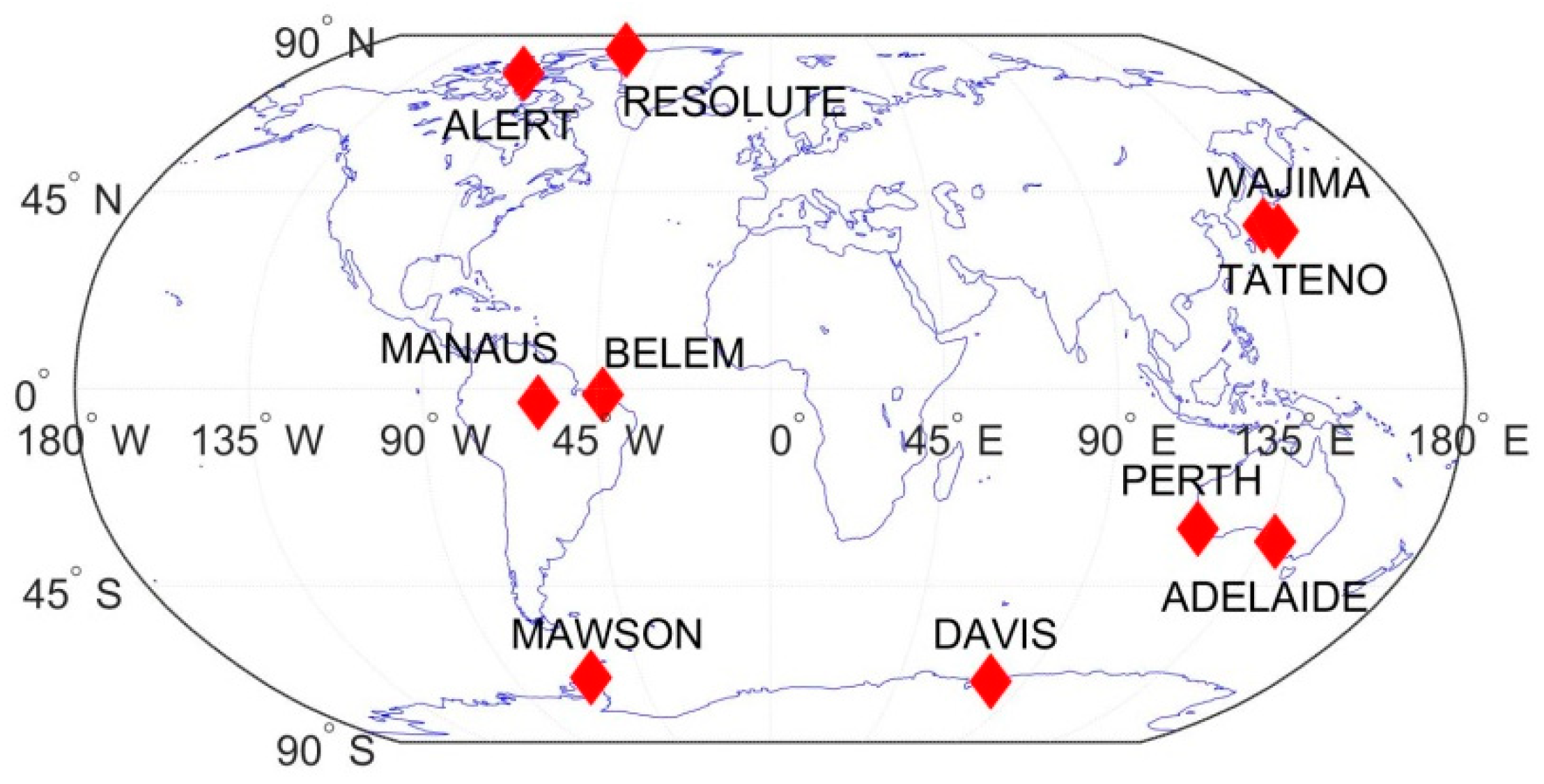
This paper is arranged as follows. Section 2 introduces data and methodology used in this research. Section 2.1 introduces RO 1DVar moist profiles and the background data used at all centers. Section 2.2 introduces the IGRA Version 2 (IGRA2) used and the detail information of the 10 stations that we selected. Section 2.3 introduces how we design our evaluation. Section 3 illustrates the results of this research and the discussions of the results are given in Section 4. Finally, a conclusion is given in Section 5.

2. Data and Methodology

2.1. RO 1DVar Retrieved Temperature and Specific Humidity Profiles

This sub-section introduces RO data types and versions from all centers that we used for our calculation. The methodology of each centers 1DVar retrieval processes and also uncertainty settings are also briefly introduced in this setting based on the latest literature that we can find online.

2.1.1. WEGC Profiles

We use WEGC provided RO level-2 profiles including both dry atmospheric profiles and moist profiles. We therefor use their level-2 profiles for our evaluation. The data version is the latest processed data using its Occultation Processing System version 5.6 [35,36,37]. The background data used for producing these moist profiles are ECMWF operational 24 h forecast fields collocated to the locations of RO events.

WEGC’s moist profiles are processed using its Occultation Processing System version 5.6 [35,37]. Currently, WEGC provides RO level-2 profiles including both dry atmospheric profiles and moist profiles.

At WEGC, a simplified linear 1DVar-alternative method, is used to produce its moist profiles [21,24]. It uses RO retrieved dry temperature as the main observed input. The dry temperature uncertainties are modelled following the empirically derived error model developed by Scherllin-Pirscher et al. [37] with different parameter value settings. Currently, the model is designed to only have vertical variation currently. Above 10 km, temperature uncertainties are about 0.7 K. Below 10 km, uncertainties increase and reach about 4 K at bottom altitude levels.

Uncertainties of background temperature and specific humidity are estimated just using the empirical uncertainty profile of ECMWF. The background temperature uncertainties are about 0.8 K from 3 to 10 km. Below 3 km, uncertainties increase with decreasing altitude to more than 1 K at the surface. From 10 km upwards, uncertainties increase to 2K at 16 km, which is the highest level of WEGC moist processing. Background specific humidity uncertainty is 10% at the surface, increases to about 40% at 7 km, and then gradually decreases to about 15% at 16 km. The vertical correlations of background and also observations are currently ignored at WEGC since they are found to be small with correlation lengths that are generally less than 1 km for most cases. The details of these uncertainty estimations and values are given in detail by Li et al. [24].

The moist air retrieval is only applied up to an altitude of 16 km, with a half-sine-weighted transition from moist to dry parameters between 14 and 16 km for temperature and pressure. This signifies that at 14 km and below, only information from the optimal estimation retrieval enters the profiles, while at 16 km and above, moist and dry parameters are identical to within 0.01 K.

2.1.2. ROM SAF Profiles

We use the ROM SAF latest reprocessed Climate Data Records CDRv1.0 for calculation [38]. The CDRv1.0 processing is based on ROPP 8.1, with few adaptations [39,40]. The file type “wet” provides RO moist profiles and “bgf” provides the collocated background profiles that are used as inputs for 1DVar. The background files “bgf” are obtained from ERA-Interim forecast fields. For each occultation event, the background temperature, specific humidity and surface pressure are spatially and temporally interpolated to the time and the location of the coming in RO event. The 1DVar configuration is defined by a few choices described in detail in the ROM SAF 2018 report on Level 2B and 2C 1DVar profiles [24]. The 1DVar validation results of ROM SAF moist profiles can be found at [41].

ROM SAF uses the conventional 1DVar approach for producing its moist profiles [23]. Refractivity is used as an observed variable [23,40]. The refractivity error covariance matrix is constructed using uncertainty profile multiplying with correlation matrix. The refractivity uncertainty estimate is 2% at the surface, decreasing linearly to 0.2% at the tropopause. Above the tropopause, the fractional uncertainties are 0.2% or 0.02 N-units. Refractivity vertical correlations are assumed to be exponential with a 3 km correlation length. The background error covariance matrix is constructed using one-dimensional uncertainty profile combined with an error correlation matrix. The correlation matrix C is constant and is provided by ECMWF and used by interpolation in ROM SAF 1DVar process. In estimating background uncertainties, a static temperature uncertainty and a static relative specific humidity uncertainty is formed by using the uncertainty estimated directly provided by ERA-I forecast data. Then the background uncertainties are estimated as standard deviations of the collocated background profile against a set of ERA-I files ranging over the whole CDR-v1.0 period. Specific humidity uncertainties are estimated by resolving a constructed uncertainty model every 5 deg and RO events within a band just using the estimated uncertainties within the band. More details about the uncertainty estimations can also be found at the ROM SAF 1DVar report [23].

2.1.3. UCAR Profiles

RO observables used as inputs are refractivity. UCAR’s profiles can be found online at [42]. The file type “wetPrf’ contains its 1DVar profiles including temperature and specific humidity. In this study, its latest reprocessed version 2013.2350 is used (accessed on March 2020). The background data used at UCAR are ECMWF low resolution analysis fields. The file type “ecmPrf” provides the collocated background profiles that were used for 1DVar retrieval [42].

UCAR also uses the conventional 1DVar approach to produce moist profiles [20]. According to an early report by COSMIC project office [20], the observation and background error covariance matrices are also constructed by using one-dimensional uncertainty profile combined with an error correlation matrix. The observation uncertainties include both systematic and random components, which are latitude-dependent and are estimated from the statistics of innovation vectors for a reasonably long period such as 1 month, and the information was updated regularly from the statistics for a recent period to yield best-possible performance. The estimation of the background uncertainties at CDAAC is similar to the estimation of observation uncertainties. The correlation matrix was estimated using a fifth-order correlation function, such as used by Steiner and Kirchengast [43], which is similar to a Gaussian function in shape.

2.2. IGRA2 Radiosonde Data

Radiosonde data from the IGRA2 are compared to RO data in this study and these data can be found at the website of NCDC NOAA at [44]. IGRA2 replaces IGRA1 as American National Climatic Data Center (NCDC) baseline upper-air dataset [45]. Compared to IGRA1, IGRA2 contains data from nearly twice as many stations and 30% more soundings. Furthermore, it provides longer data records with more variables and also includes data from ships and ice islands. From IGRA2 profiles, we use the IGRA-Derived sounding parameter files, which are available for a subset of the soundings in IGRA. We use temperature, pressure and water vapor pressure in our comparison.

In selecting RS stations, we have several criteria. First of all, the stations are required to be distributed in different latitudinal bands, which can reflect the influences of water vapor on the RO retrievals; secondly, the stations should continuously provide RS measurements over the period from 2007 to 2010 when COSMIC mission provides dense observations; thirdly, stations should use the same radiosonde type and sensors to avoid uncertainties brought in by instruments. Based on these criteria, we select 10 stations distributed in five latitudinal bands of 60°–90°N, 20°–60°N, 20°S–20°N, 20°–60°S, and 60°–90°S. For each latitudinal band, the two stations selected are in relatively close distance and sharing the same radiosonde type and sensors. The radiosonde types selected for these 10 stations are either Meisei or Vaisala, which have been proven to be of high quality by several studies [28,46]. The locations of these 10 stations are shown in Figure 1 and the detailed information in terms of radiosonde types and station code are shown in

Table 1. Detail information of selected IGRA RS stations for comparison, the final five digital numbers of the station code are the WMO identification number of each station.

Lat Band	Station Name	Station Code	Location (lat°/lon°)	Radiosonde Type
60°–90°N	RESOLUTE	CAM00071924	74.72/−94.38	VAISALA RS80
	ALERT	CAM00071082	82.5/−62.33
20°–60°N	WAJIMA	JAM00047600	37.4/136.9	MEISEI RSII-91
	TATENO	JAM00047646	36.05/140.13
20°S–20°N	BELEM	BRM00082193	−1.38/−43.48	VAISALA RS80
	MANAUS	BRM00082332	−3.15/−59.98
20°S–60°S	PERTH	ASM00094610	−31.9/116.0	VAISALA RS92K
	ADELAIDE	ASM00094672	−34.95/138.533
60°S–90°S	MAWSON	AYM00089564	−67.6/62.9	VAISALA RS92-SGP
	DAVIS	AYM00089571	−68.6/78.0

.

2.3. Methodology

In this study, we evaluate only temperature and specific humidity profiles. Other parameters, such as pressure, water vapor volume and mixing ratio can be directly calculated using these two parameters together with moist air gas constant ratio parameters and also dry pressure [24]. Therefore, the characteristics of these other parameters would be similar to the two parameters and are not discussed here. We select profiles of COSMIC mission for our evaluation. The selected data period is from 2007 to 2010 when COSMIC mission has dense global observations.

The first step of our comparison is to match RO and RS observations. We collocated RO and RS profiles by matching the positioning of the RS launch station to the mean tangent point of RO, and the launch time of RS to the mean event time of RO. The collocation criteria are 2 h and 200 km, which is a moderate criterion [25,28]. Based on matched pairs, we interpolate RO profiles on 11 selected standard pressure layers of RS from 925 hPa to 50 hPa using logarithmic interpolation [25,32]. These standard pressure layers are defined in IGRA2 and can be seen from our results sections where standard layers are marked. Based on the interpolated profiles, we calculate temperature difference ΔT and relative specific humidity difference Δq:

$$\mathsf{\Delta }T=T_{\mathrm{RO}}-T_{\mathrm{RS}}$$

(2)

$$\mathsf{\Delta }q=\left(q_{\mathrm{RO}}-q_{\mathrm{RS}}\right)/{\overline{q}}_{\mathrm{RS}}\times 100$$

(3)

where T_RO and q_RO represent RO temperature and specific humidity, respectively; T_RS and q_RS represent matched RS temperature and specific humidity, respectively; and ${\overline{q}}_{\mathrm{RS}}$ represents mean RS specific humidity of all used samples, and it is used to avoid the small number of specific humidity in the upper troposphere exaggerating the percentage. Mean difference profiles of multiple stations are just obtained by averaging profiles of all matched profiles at each station and corresponding standard deviations are obtained by using the obtained mean difference profiles and the complete difference profiles of all stations.

In order to make sure that good quality data is used for comparison, we apply a quality control procedure following the experience found by Ladstädter et al. [25]. First, we process and check the RS profiles independently. We reject each profile that contains overly large vertical gaps between adjacent levels in a defined “core region” from 600 to 200 hPa. The maximum inter-level gap is 2 km for temperature and 4 km for specific humidity. If the humidity profile is rejected according to these criteria, but the temperature profile passes, we keep the temperature profile for further processing, and the same in a round way. Furthermore, if large gaps are found outwards of the defined core region, the profile is cut from the first gap. Secondly, RO profiles are checked individually by using the quality flag provided by each center. We only use RO profiles in which all centers show good quality.

Based on the high quality difference profiles, we calculate statistical differences between RO retrieved profiles and RS and the differences between background and RS over selected spatial and temporal domain. First of all, we calculate 4 years’ mean differences between RO and RS for stations located in the five latitudinal bands described above and also for all the 10 stations located in the whole globe. We then calculate 4 years’ mean differences between background profiles and RS with corresponding standard deviations to investigate the agreements between background profiles and RS. To further understand how the background data influences RO retrieved moist profiles, we compare the differences between RO and RS with the differences between background and RS. Finally, we calculate mean differences and standard deviations over selected pressure layers every 3 months to investigate temporal variability of these profiles.

3. Results

3.1. Four Year Mean Statistics at Six Stations

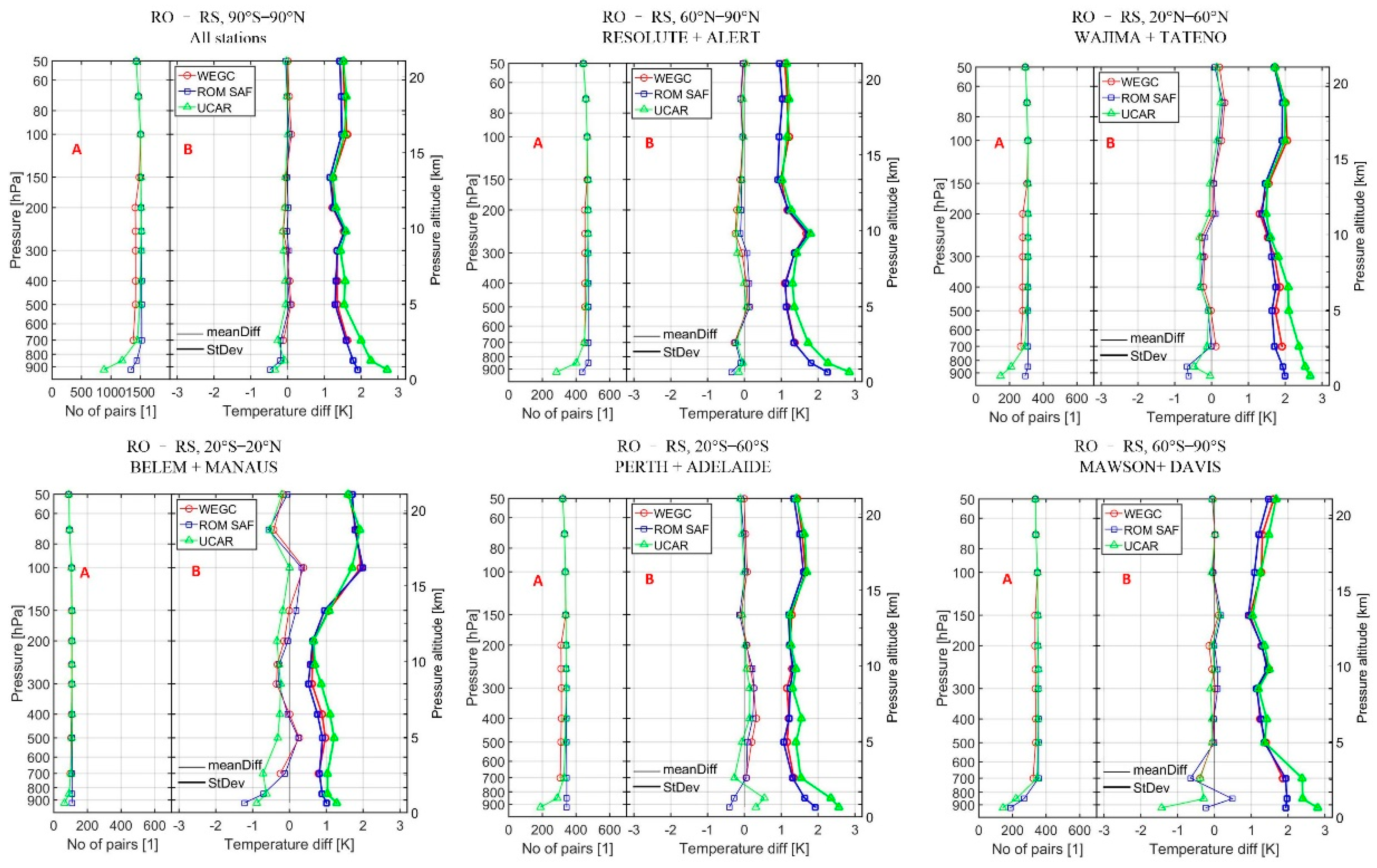
Figure 2 shows temperature mean differences between RO and RS and the corresponding standard deviations over the period of 2007 to 2010 at stations located in different latitudinal bands. Results of WEGC, ROM SAF and UCAR centers are all shown. The numbers of used paired samples at all pressure levels are also indicated in sub-panels A. From the first row to second row, the six panels show statistical results at stations over latitudinal bands of 90°S–90°N, 60°–90°N, 20°–60°N, 20°S–20°N, 20°–60°S, and 60°–90°S, respectively. The markers of all lines represent the standard RS pressure levels that we used for interpolation of RO profiles (c.f., Section 2.3). The pressure altitude P_altitude is an approximate altitude level calculated as $P_{\mathrm{altitude}}=-H_0\ln \frac{p}{p0}$, where H₀ = 7 km is the tropospheric scale height, p is atmospheric pressure and is the standard pressure level in this study, and p₀ = 1013.25 hPa is the standard surface pressure. The pressure altitude is used as an approximate altitude estimate auxiliary for checking the corresponding altitude of a given pressure level.

From sub-panel A of this figure, we can see that the number of matched pairs of all stations is about 1500. The numbers of paired samples of the stations in the two polar bands are largest with values around 400. The number of stations in two mid-latitudinal bands is around 300. The matched numbers are smallest at tropical stations due to smaller density of COSMIC RO events in tropical regions [5]. RO data of WEGC are usually missing at the lowest pressure levels. This is because WEGC center chooses to cut profiles higher above the surface than the other two centers [36].

Comparing temperature differences of stations in different latitudinal bands, we find that the differences are smallest at polar stations and gradually increase with the decrease of latitude and are found to be largest at tropical stations. This is mainly because the polar region has a smaller water vapor amount. RO measurements suffer less from water vapor ambiguity as well as multipath issues and the differences against RS are be smaller. At the middle and especially tropical stations, where a larger amount of water vapor exists, RO measurements are suffered from multipath and other measurement uncertainties and also then agree less with RS.

For the results of all 10 stations, temperature mean differences are varying within ±0.1 K at altitudes above 500 hPa, while at altitudes below 500 hPa, mean differences are varying within ±0.5 K. Temperature standard deviations of the three centers are similar at altitudes above 300 hPa with values varying within 1–1.5 K. At altitudes below 300 hPa, standard deviations increase with the decrease of height, with values of WEGC and ROM SAF varying within 1–2 K; and values from UCAR are the largest, with values varying from 1 to 3 K.

At the stations located in the two polar latitudinal bands of 60°–90°N and 60°–90°S, temperature differences between RO and RS of the three centers are similar with values varying within ±0.2 K for most pressure levels. Larger differences are found at the southern hemisphere polar stations MAWSO and DAVIS with values varying within ±0.8 K below 500 hPa. Temperature standard deviations of WEGC and ROM SAF are similar with values varying from 1 K at 50 hPa to 2 K at bottom pressure levels. Standard deviations of UCAR are larger than that of the other two centers at altitudes below 500 hPa, with values exceeding 3 K at bottom pressure levels.

At the stations located in the two mid-latitudinal bands of 20°–60°N and 20°–60°S, mean differences are larger than that at the two polar stations, with values varying within ±0.5 K for most pressure levels. From 500 to 200 hPa, the differences of stations in the latitudinal band of 20°–60°N are negative varying from −0.5 to 0 K, while the differences of the stations in the band of 20°–60°S over the same pressure layer are positive, with values varying from 0 to 0.5 K. Mean differences of all three centers are overall similar with ±0.5 K variations below 700 hPa. Standard deviations of WEGC and ROM SAF are very similar at all pressure levels, with values varying from 1 to 2 K. Standard deviations of UCAR are larger than that of the other two centers from 400 hPa to the surface, with values reaching 3 K at bottom pressure levels.

Mean differences of the stations located in the tropical band were the largest compared with stations in mid- and high latitudinal bands. Mean differences of WEGC and ROM SAF are similar with values varying from −1 to 0.2 K. Mean differences of UCAR at altitudes below 400 hPa are 0.5 K larger (in absolute terms) than that of WEGC and ROM SAF. Standard deviations from all three centers are overall similar for most pressure levels with values varying from 1 K at bottom pressure levels to more than 3 K at higher pressure levels.To further quantify temperature mean differences and also standard deviations shown in Figure 2, we summarize the values at 200, 400 and 700 hPa, representing high, middle and low troposphere in

Table 2. Temperature mean differences (meanDiff) and corresponding standard deviations (StDev) between RO and RS of the three centers at selected pressure levels of 200, 400 and 700 hPa.

Lat Band Station	Pressure Level [hpa]	Temperature meanDiff (StDev) [K]
		WEGC	ROM SAF	UCAR
90°S–90°N All stations	200	−0.07(1.22)	0.02(1.24)	−0.08(1.31)
	400	0.05(1.34)	0.01(1.31)	−0.06(1.56)
	700	−0.12(1.62)	−0.19(1.58)	−0.27(1.99)
60°N–90°N RESOLUTE ALERT	200	−0.20(1.17)	−0.08(1.19)	−0.17(1.27)
	400	0.06(1.10)	0.13(1.12)	−0.01(1.30)
	700	−0.26(1.37)	−0.24(1.35)	−0.21(1.73)
20°S–60°N WAJIMATA TENO	200	0.04(1.31)	0.10(1.37)	−0.06(1.48)
	400	−0.22(1.85)	−0.29(1.75)	−0.30(2.08)
	700	0.12(1.91)	−0.01(1.71)	−0.12(2.37)
20°S–20°N BELEM MANAUS	200	−0.14(0.65)	−0.04(0.64)	−0.34(0.66)
	400	0.002(0.89)	−0.05(0.76)	−0.26(1.10)
	700	−0.25(0.80)	−0.12(0.82)	−0.72(1.04)
20°S–60°S PERTH ADELAIDE	200	0.07(1.24)	0.04(1.23)	0.03(1.26)
	400	0.32(1.21)	0.23(1.22)	0.14(1.55)
	700	0.05(1.34)	0.05(1.31)	−0.27(1.53)
60°S–90°S MAWSON DAVIS	200	−0.14(1.27)	−0.001(1.29)	−0.05(1.36)
	400	−0.03(1.24)	−0.02(1.27)	−0.07(1.42)
	700	−0.40(1.86)	−0.65(1.93)	−0.39(2.38)

. It can be seen from the table that the discrepancies between WEGC and ROM SAF measurements are overall small at all pressure levels with discrepancies of mean differences between the two centers varying within 0.05 K and standard deviations varying within 0.1 K for most cases. Standard deviations of UCAR at 700 hPa are 0.5 to 1 K larger than that of other two centers for these selected stations.

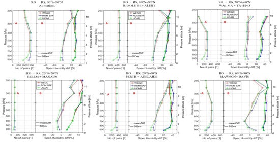
Figure 3 shows specific humidity mean differences between RO and RS and corresponding standard deviations of all three centers over the same period from 2007 to 2010 at stations located in the six latitudinal bands. Figure layout is the same as Figure 2. From subpanels A of this figure, we can see that the numbers of matched samples are overall similar to temperature results. However, matched pairs decrease at altitudes above 400 hPa for stations in 20–60°N band. This is because RS measurements are missing for these two stations above 400 hPa.

Results at different latitudinal bands show no strong latitudinal variations. For most RS stations, RO specific humidity shows overall positive differences at altitudes above 600 hPa, indicating more moisture retrieval of RO than RS. For stations in the 90°N–90°S band, mean differences vary from −5% at bottom pressure levels to about 20% at 200 hPa. For stations in the latitudinal bands of 60°N–90°N, 20°S–20°N, 20°S–60°S, and 60°S–90°S, magnitudes of mean differences are similar with negative values varying from −5% to −10% at altitudinal levels below 600 hPa to about 40% at uppermost pressure levels. Standard deviations are varying from 20% to 40%. For the two stations in 20°N–60°N, which used the MEISEI RSII-91 RS type, mean differences are rather small with values varying within ±5%, while standard deviations are still varying from 20% to 40%. To quantify mean differences and corresponding standard deviations of RO specific humidity, we summarize the values at 200, 400 and 700 hPa of all centers in

Table 3. Specific humidity mean differences (meanDiff) and corresponding standard deviations (StDev) between RO and RS of the three centers at selected pressure levels of 200, 400 and 700 hPa.

Lat Band Station	Pressure Level [hpa]	Specific Humidity meanDiff (Stdev) [%]
		WEGC	ROM SAF	UCAR
90°S–90°N All stations	200	18.60(34.81)	17.34(34.15)	20.93(33.99)
	400	7.56(27.92)	6.00(27.95)	4.97(28.60)
	700	−2.35(27.03)	−1.49(28.34)	−3.77(28.55)
60°N–90°N RESOLUTE ALERT	200	13.11(36.02)	16.14(39.3)	17.80(40.24)
	400	11.10(33.62)	11.88(35.10)	9.83(33.23)
	700	1.43(28.92)	1.49(29.12)	0.44(27.16)
20°S–60°N WAJIMATA TENO	200	-	-	-
	400	3.62(28.30)	0.03(30.28)	−1.71(29.79)
	700	−2.13(31.06)	−1.45(33.41)	−5.85(30.48)
20°S–20°N BELEM MANAUS	200	37.55(45.62)	29.16(49.48)	30.92(50.29)
	400	7.95(45.51)	6.28(45.52)	6.06(44.71)
	700	−8.53(25.59)	−9.47(26.34)	−10.82(26.38)
20°S–60°S PERTH ADELAIDE	200	44.26(33.20)	31.50(39.18)	36.19(33.91)
	400	15.66(37.07)	11.20(40.26)	13.96(35.83)
	700	−1.99(37.03)	1.37(39.36)	−0.60(38.36)
60°S–90°S MAWSON DAVIS	200	9.09(37.09)	13.80(37.70)	16.54(38.44)
	400	5.96(36.87)	13.23(37.35)	8.40(34.59)
	700	−10.82(34.34)	−12.72(35.13)	−11.74(34.13)

.

3.2. Influences of Background

Figure 4 shows the mean differences between collocated background temperature profiles used for 1DVar retrieval and RS profiles over the same period from 2007 to 2010. Figure layout and the numbers of paired samples are the same as Figure 2. For stations located in the polar and mid-latitudinal bands, mean differences are varying within ±0.5 K for most pressure levels. Mean differences of background profiles from ROM SAF and UCAR are similar with discrepancies among the two centers within 0.1 K for most pressure levels. Background profiles from WEGC are overall 0.2 – 0.5 K larger (in absolute terms) than that of the other two centers at altitudinal levels above 200 hPa. This indicates that the operational ECWMF forecast profiles used at WEGC deviate more from RS than the ERA-Interim forecast data used at ROM SAF and the ECMWF analysis data used at UCAR above 200 hPa. Standard deviations at all stations are varying within 1 to 2 K with values above 200 hPa from WEGC are 0.2 K and 0.5 K larger than that used at other two centers.

For stations in the tropical band, mean differences are negative for most pressure levels, indicating background profiles are generally cooler than RS measurements. Mean differences are varying from −1 to 0.2 K for most pressure levels. Comparing results among centers, we can find that the discrepancies of mean differences are within 0.5 K. Standard deviations from all centers are varying from 1 to 2 K, with values from WEGC 0.5 K larger than that of other two centers at altitudinal levels above 100 hPa.

Figure 5 shows specific humidity mean differences and standard deviations between collocated background profiles and RS of the three centers. An overall look at this figure suggests that the differences between background profiles and RS are overall positive at altitudinal levels above 600 hPa for most stations except for the two stations in the 20°–60°N band, using the MEISEI RSII-91 radiosonde type. The magnitudes of these differences profiles are similar to the differences of RO profiles. Comparing the discrepancies among centers, we can find that background profiles of WEGC, ROM SAF and UCAR are overall similar with discrepancies of both mean differences and standard deviations that are within 5%.

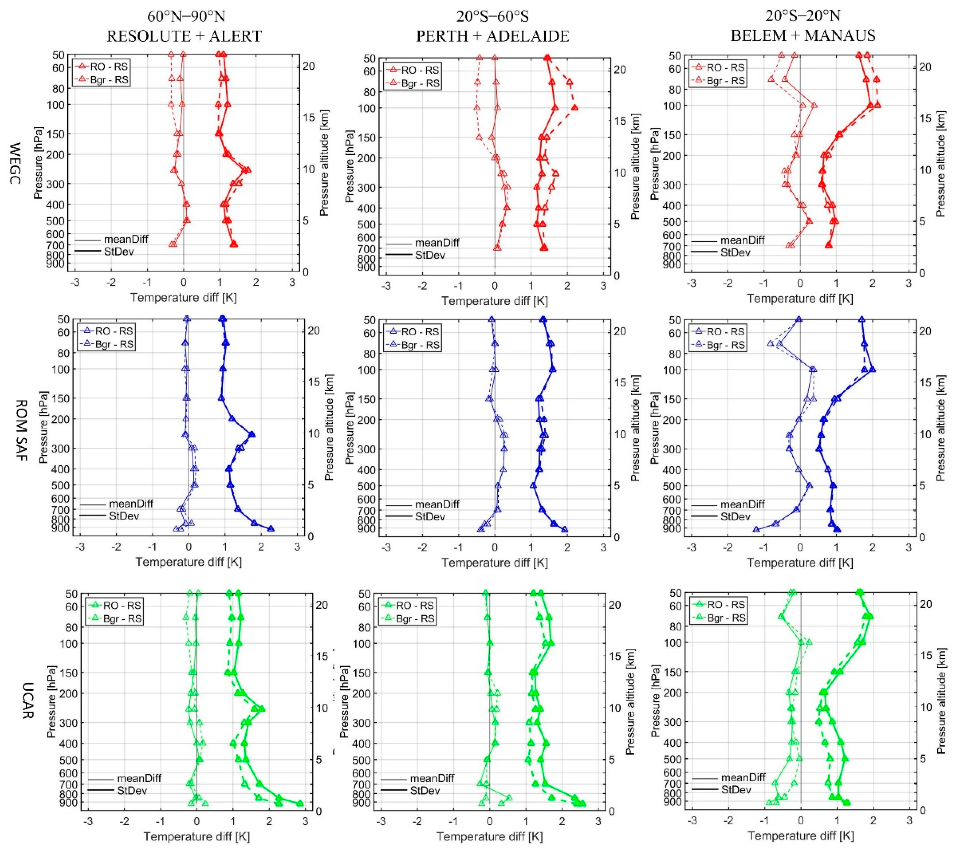
In order to further investigate how background data influences the RO retrieved moist profiles, we select stations in three latitudinal bands, 60°–90°N, 20°–60°S and 20°S–20°N to show the differences between RO and RS (RO-RS) and the differences between background and RS (Bgr-RS) in the same panel to investigate the discrepancies between RO and Bgr profiles. Figure 6 and Figure 7 show the results of temperature and specific humidity, respectively. Figure 6 shows that RO-RS of WEGC are always smaller than that of Bgr-RS over all pressure levels. The discrepancies between RO-RS and Bgr-RS are close to zero at altitudes below 200 hPa. Discrepancies increase with height, and the values are 0.2 K for stations in 60°–90°N and 20°S–20°N bands and are 0.5 K in 20°–60°S band. Li et al. [24] show that WEGC chose to use more information from observation in retrieved temperature profiles above 10 km (about 250 hPa) and more information from background below. These results together suggest that background profiles used by WEGC deviate more from RS above 200 hPa than RO observed temperature (calculated using RO observed dry temperature prescribing with specific humidity in WEGC case). Since more weights were given to the observation information from the RO measurement above 200 hPa, the retrieved optimal estimated temperature profiles are also closer to RS profiles than the background profiles.

ROM SAF retrieved temperature profiles have the smallest discrepancies against their background profiles, compared to the other two centers. For stations in polar latitudinal bands, RO-RS and Bgr-RS are similar at altitudes above 300 hPa At altitudes below 300 hPa, the discrepancies between RO-RS and Bgr-RS are within 0.2 K. For stations in mid-latitudinal bands, RO-RS and Bgr-RS are also similar. For stations in the tropical band, the discrepancies between RO-RS and also Bgr-RS at altitudes between 50 to 200 hPa are within 0.2 K, and at altitudes below 200 hPa, the discrepancies are close to zero.

UCAR results suggest that the discrepancies between RO and Bgr profiles are largest compared to the other two centers. At altitudes below 200 hPa, both mean differences and also standard deviations of Bgr-RS are smaller than that of RO-RS for most pressure levels. This indicates that the background profiles used agree more with RS than its retrieved temperature profiles. The discrepancies between RO-RS and Bgr-RS profiles above 200 hPa are overall within 0.1 K, while that at altitudes below 200 hPa are varying from 0.2 to 0.5 K, which are much larger than the discrepancies between RO and Bgr for WEGC and ROM SAF. Based on these results and also our previous internal analysis on the obr-to-bgr weighting ratio, UCAR decides to give a heavy weight to observation in optimal estimation at all pressure levels for retrieval. However, RO observations below 300 hPa usually agree less with RS and therefore the subsequently retrieved temperature profiles agree less with RS. This could help to explain why in Figure 2 temperature differences and standard deviations from UCAR are larger than that of the other two centers. However, this does not mean that results from UCAR are not accurate, but depends on the decision of centers of which climatology to as background information, and the weights of background and observation information in the optimal estimation process.

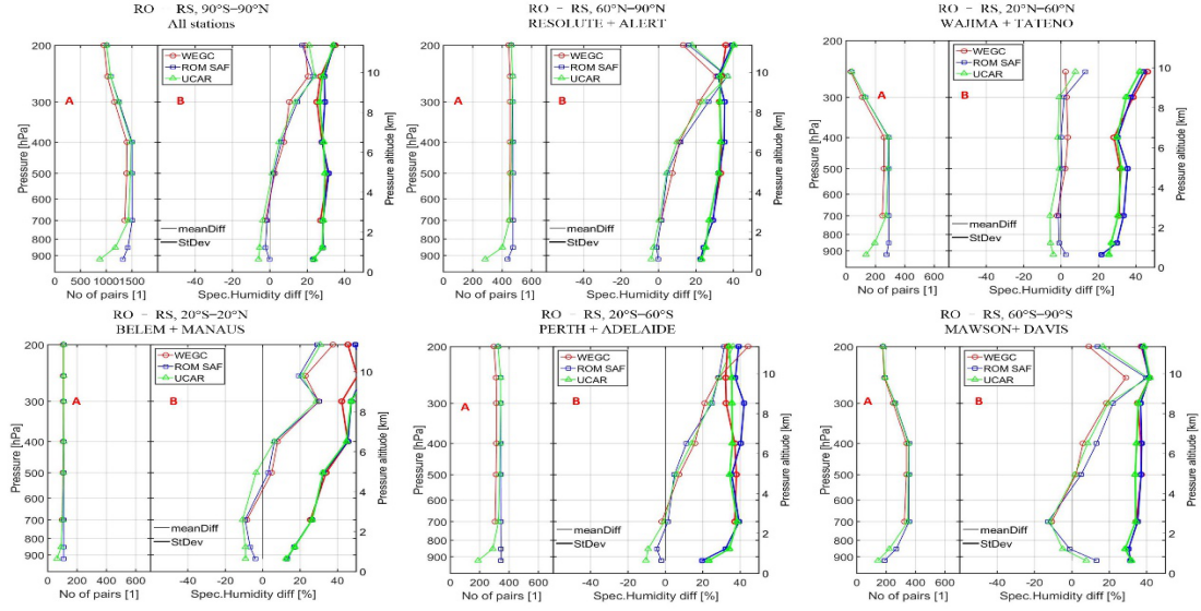
Figure 7 shows specific humidity mean differences and standard deviations of RO-RS and also Bgr-RS. Figure layout is the same as Figure 6. It can be seen from this figure that both RO-RS and Bgr-RS show large positive differences up to 40% above 300 hPa. Since Li et al. [24] found that RO retrieved specific humidity use more information from background above about 7 km, therefore, these large positive differences are related to the used background profiles. However, further efforts are required to investigate the differences between RO temperature (dry temperature in WEGC case and forward propagated temperature in the conventional 1DVar case) and RS. For stations in the 60°―90°N band, the discrepancies of both mean differences and standard deviations between RO-RS and Bgr-RS are within ±2%. For stations in the 20°–60°S band, discrepancies of mean differences between RO-RS and Bgr-RS are within 2% for most pressure levels, while discrepancies of standard deviations vary from 2% to 5%. Comparing discrepancies between centers within this band, WEGC shows the smallest discrepancies, while ROM SAF results are the largest discrepancies between RO and Bgr. For stations in the tropical band, discrepancies of mean differences between RO-RS and Bgr-RS are within 10% for most pressure levels, and discrepancies of standard deviations are within 5% for most cases. Within this latitudinal band, rprofiles from WEGC show the largest discrepancies, while that from ROM SAF show the smallest discrepancies.

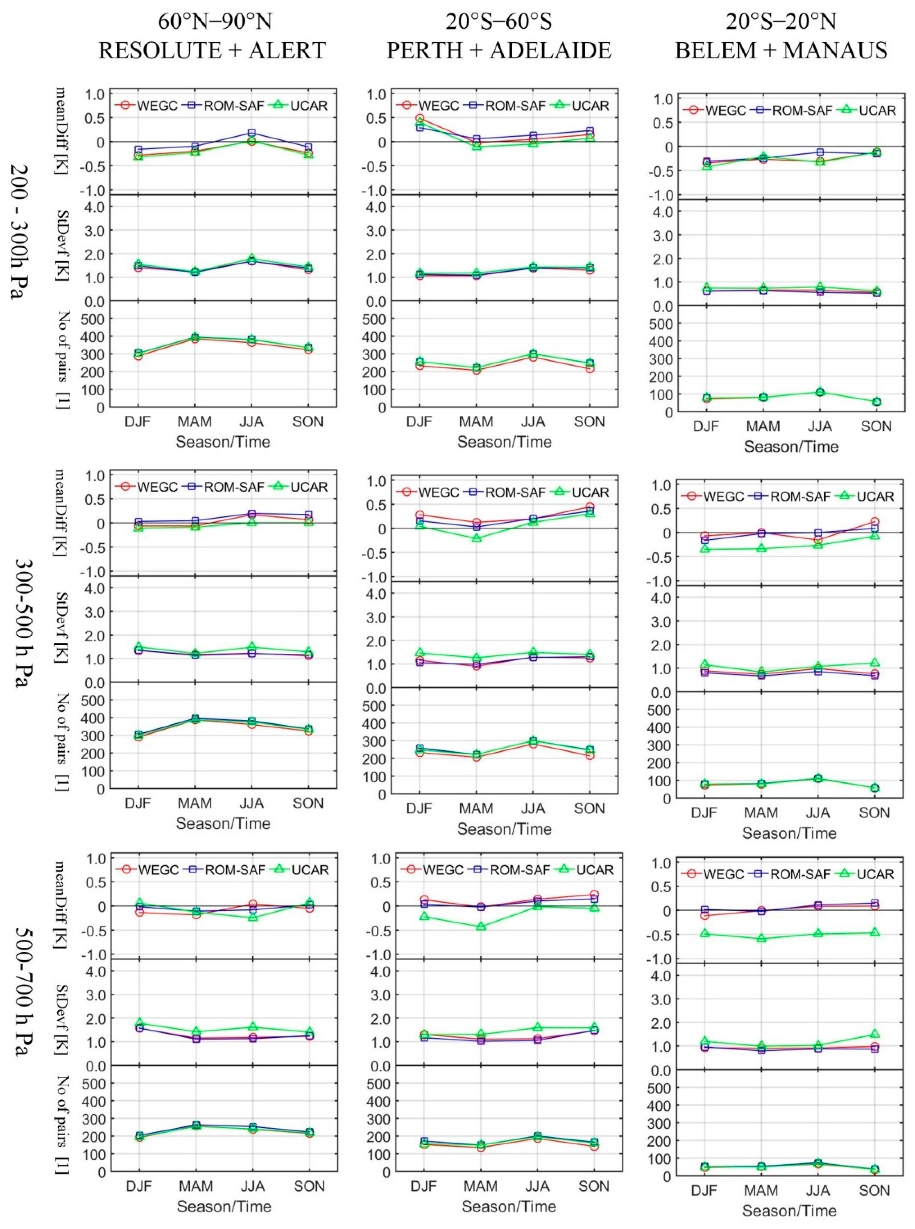
3.3. Temporal Variability

We divided the whole year into four temporal phases, i.e., December, January and February (DJF); March, April and May (MAM); June, July and August (JJA); and September, October and November (SON). These four temporal phases represent different seasons of either winter or summer for middle and high latitudinal stations. For tropical stations, which only have dry and wet seasons, these four temporal phases only used to show temporal variations. For each season, we calculate mean differences and corresponding standard deviations between RO and RS over three selected pressure layers from 200–300 hPa, 300–500 hPa and 500–700 hPa. These three pressure layers represent the high, middle and low tropospheric layers. We select stations in the three latitudinal bands, 60°–90°N, 20°–60°S and 20°S–20°N to show the temporal variations of temperature and specific humidity differences.

Figure 8 shows the temporal variability for temperature profiles. Small variability is found for different temporal phases with variations generally within 0.5 K. Temperature differences of UCAR in tropical stations over 500–700 hPa are found to be overall 0.5 K larger (in absolute terms) than that of the other two centers. This can be related to the heavy weight given to RO observation at low pressure levels, which agree less with RS. Figure 9 shows the temporal variability for specific humidity profiles. It can be seen that specific humidity also shows small temporal variability for stations in the latitudinal bands of 60°–90°N and 20°–60°S. However, specific humidity standard deviations at stations in the tropical band are found to have visible variations with the values in JJA and SON temporal phases 5% to 20% larger than that of other seasons.

4. Discussion

Results of Section 3 suggest that RO 1DVar retrieved temperature profiles from WEGC, ROM SAF, and UCAR data processing centers are overall similar in different selected spatial and temporal phases. Some discrepancies are found for temperature below 300 hPa where temperature standard deviations of UCAR are 0.5–1 K larger than the other two centers. We investigate this discrepancy by comparing the background temperature profiles used at all centers. It is found that background profiles used at all centers are similar below 300 hPa. These findings together with the obs-to-bgr weighting ratios found by Li et al. [24] suggest that the 0.5–1 K larger standard deviations can be related to a heavy weight given to RO observation information, which agrees less with RS at altitudes below 300 km. The differences of RO retrieved refractivity can also influence the 1DVar retrieved profiles. However, these influences are considered to be minor since several studies and also our internal analysis suggest that refractivity profiles from different centers are overall consistent down to 5 km [47,48].

Specific humidity from RO and background profiles used show 40% positive differences at altitudinal levels above 600 hPa for most selected stations. These results are similar with the findings from Ladstädter et al. [25], Rietch et al. [27] and the ROM SAF validation report [41]. Comparison between background profiles with RS profiles found that background profiles also have these strong positive differences. Considering all centers choose to use more background information in the retrieved specific humidity at altitude levels above 400 hPa, these positive differences can influence the positive differences found in the retrieved specific humidity profiles. However, further efforts are required to investigate the differences between RO humidity information and RS humidity profiles by using forward propagation.

This research only initially discusses the origin of the discrepancies of moist profiles among centers by comparing the discrepancies of RO retrieved profiles and background profiles. However, since the uncertainties are not fully provided by centers yet and the conventional 1DVar is not a linear process, some aspects of the discrepancies of moist profiles among centers are still unclear. Further efforts should be carried out by investigating the weighting of background and observation information in their retrieved profiles. This requires data centers to provide the uncertainties of observed and background profiles. Then users can understand how much observed and background information were used in their retrieved moist profiles and can help them to explain weather and climate phenomena. Furthermore, more stations are required to be selected in future to represent the full climatological condition of a latitude band.

Finally, and also importantly, we show the differences of WEGC, ROM SAF and UCAR data processing centers by comparing their 1DVar products with RS. However, we did not indicate the accuracy of any center for several reasons: (1) Many existing studies have proven that all centers show similar and high quality RO refractivity profiles, indicating the robustness of retrieval capability of the three centers; (2) The decisions of centers on how to weight background and observation information can make the results different; (3) RS measurements are also not truth and have intrinsic systematic biases. Further efforts are required to compare moist profiles from more independent datasets and to analyze the differences in uncertainty estimations.

5. Conclusions

This study evaluates RO moist profiles including temperature and specific humidity from WEGC, ROM SAF and UCAR data processing centers by comparing measurements from 10 selected IGRA2 radiosonde stations distributed in different latitudinal bands. The origins of the discrepancies are also briefly discussed by comparing background profiles with RS profiles. RO retrieved temperature profiles from all centers agree well with radiosonde. Mean differences at polar, mid-latitudinal and tropical stations are varying within ±0.2 K, ±0.5 K and from −1 to 0.2 K, respectively, with standard deviations varying from 1 to 2 K for most pressure levels. The differences between RO retrieved and the background temperature profiles for WEGC are varying within ±0.5 K at altitudes above 300 hPa, and the differences for ROM SAF are within ±0.2 K for all pressure levels, and that for UCAR are within 0.5 K at altitudes below 300 hPa. RO retrieved temperatures from all three centers are overall similar at altitudes above 300 hPa. Discrepancies among centers are found below 300 hPa. Heavy weights of RO observation can lead to larger differences since RO observations are found to agree less with RS than the background temperature profiles used at the three centers.

Both RO retrieved and background specific humidity above 600 hPa are found to have large positive differences (up to 40%) against most RS measurements, and the positive differences in RO retrieved specific humidity is related to the background specific humidity used. Discrepancies of moist profiles among the three centers are overall minor at altitudes above 300 hPa for temperature and at altitudes above 700 hPa for specific humidity. Specific humidity shows the largest standard deviations at tropical stations in June–July–August months.

In future, we will carry on our research to further expand our findings by selecting more RS stations in all latitudinal bands representing complete atmospheric features in each latitudinal band. We will also compare RO 1DVar retrievals with other independent datasets, such as GRUAN. We will also investigate the obs-to-bgr weighting ratios to determine the origins of the discrepancies among centers.

References

1. Melbourne, W.G. The application of spaceborne GPS to atmospheric limb sounding and global change monitoring. JPL Publ. 1994, 147, 1–26. [Google Scholar]
2. Kursinski, E.R.; Hajj, G.A.; Schofield, J.T.; Linfield, R.P.; Hardy, K.R. Observing Earth’s atmosphere with radio occultation measurements using the Global Positioning System. J. Geophys. Res. 1997, 102, 23429–23465. [Google Scholar] [CrossRef]
3. Hajj, G.A.; Kursinski, E.R.; Romans, L.J.; Bertiger, W.I.; Leroy, S.S. A technical description of atmospheric sounding by GPS occultation. J. Atmos. Sol. Terr. Phys. 2002, 64, 451–469. [Google Scholar] [CrossRef]
4. Kirchengast, G. Occultations for probing atmosphere and climate: Setting the scene. In Occultations for Probing Atmosphere and Climate; Kirchengast, G., Foelsche, U., Steiner, A.K., Eds.; Springer: Berlin/Heidelberg, Germany, 2004; pp. 1–8. [Google Scholar]
5. Anthes, R.A. Exploring Earth’s atmosphere with radio occultation: Contributions to weather, climate and space weather. Atmos. Meas. Tech. 2011, 4, 1077–1103. [Google Scholar] [CrossRef] [Green Version]
6. Kursinski, E.R.; Hajj, G.A.; Hardy, K.R.; Romans, L.J.; Schofield, J.T. Observing tropospheric water vapor by radio occultation using the Global Positioning System. Geophys. Res. Lett. 1995, 22, 2365–2368. [Google Scholar] [CrossRef]
7. Smith, E.K.; Weintraub, S. The constants in the equation for atmospheric refractive index at radio frequencies. Proc. IRE 1953, 41, 1035–1037. [Google Scholar] [CrossRef] [Green Version]
8. Healy, S.B.; Eyre, J.R. Retrieving temperature, water vapour and surface pressure information from refractive-index profiles derived by radio occultation: A simulation study. Q. J. R. Meteorol. Soc. 2000, 126, 1661–1683. [Google Scholar] [CrossRef]
9. Thayer, G. An improved equation for the refractive index of air. Radio Sci. 1974, 9, 803–807. [Google Scholar] [CrossRef]
10. Foelsche, U. Physics of Refractivity, in Tropospheric Water Vapor Imaging by Combination of Ground-Based and Spaceborne GNSS Sounding Data. Ph.D. Thesis, University of Graz, Graz, Austria, 1999. [Google Scholar]
11. Healy, S.B. Refractivity Coefficients Used in the Assimilation of GPS Radio Occultation Measurements; GRAS SAF Report 09; Danish Meteorol. Inst.: Copenhagen, Denmark, 2009. [Google Scholar]
12. Aparicio, J.M.; Laroche, S. An evaluation of the expression of the atmospheric refractivity for GPS signals. J. Geophys. Res. 2011, 116, D11104. [Google Scholar] [CrossRef]
13. Foelsche, U.; Borsche, M.; Steiner, A.K.; Gobiet, A.; Pirscher, B.; Kirchengast, G.; Wickert, J.; Schmidt, T. Observing upper troposphere-lower stratosphere climate with radio occultation data from the CHAMP satellite. Clim. Dyn. 2008, 31, 49–65. [Google Scholar] [CrossRef] [Green Version]
14. Ware, R.; Exner, M.; Gorbunov, M.; Hardy, K.; Herman, B.; Kuo, Y.; Meehan, T.; Melbourne, W.; Rocken, C.; Schreiner, W.; et al. GPS sounding of the atmosphere from low Earth orbit: Preliminary results. Bull. Am. Meteorol. Soc. 1996, 77, 19–40. [Google Scholar] [CrossRef] [Green Version]
15. Eyre, J.R. Assimilation of Radio Occultation Measurements into a Numerical Weather Prediction System; ECMWF Tech. Memo. No. 199; ECMWF: Reading, UK, 1994. [Google Scholar]
16. Zou, X.; Kuo, Y.-H.; Guo, Y.R. Assimilation of atmospheric radio refractivity using a non-hydostatic adjoint model. Mon. Weather Rev. 1995, 123, 2229–2249. [Google Scholar] [CrossRef] [Green Version]
17. Kursinski, E.R.; Healy, S.B.; Romans, L.J. Initial results of combining GPS occultation with ECMWF global analyses within a 1DVar framework. Earth Planets Space 2000, 52, 885–892. [Google Scholar] [CrossRef] [Green Version]
18. Palmer, P.I.; Barnett, J.; Eyre, J.; Healy, S.B. A non-linear optimal estimation inverse method for radio occultation measurements of temperature, humidity and surface pressure. J. Geophys. Res. 2000, 105, 17513–17526. [Google Scholar] [CrossRef] [Green Version]
19. Von Engeln, A.; Nedoluha, G.; Kirchengast, G.; Bühler, S. One-dimensional variational (1-D Var) retrieval of temperature, water vapor, and a reference pressure from radio occultation measurements: A sensitivity analysis. J. Geophys. Res. 2003, 108, 4337. [Google Scholar] [CrossRef]
20. COSMIC Project Office. Variational Atmospheric Retrieval Scheme (VARS) for GPS Radio Occultation Data. Report; University Corporation for Atmospheric Research: Boulder, CO, USA, 2005. [Google Scholar]
21. Kirchengast, G.; Fritzer, J.; Schwärz, M. ESA-OPSGRAS—Reference Occultation Processing System (OPS) for GRAS on MetOp and Other Past and Future RO Missions; WEGC-IGAM/UniGraz Proposal to ESA/ESTEC, Doc-Id: WEGC/ESA-OPSGRAS/Prop/v4May10; University of Graz: Graz, Austria, 2010. [Google Scholar]
22. Wee, T.-K.; Kuo, Y.-H. Advanced stratospheric data processing of radio occultation with a variational combination for multifrequency GNSS signals. J. Geophys. Res. Atmos. 2014, 119, 11011–11039. [Google Scholar] [CrossRef]
23. ROM SAF, Algorithm Theoretical Baseline Document: Level 2B and 2C 1DVar products Version 3.1 2018. Available online: http://www.romsaf.org/product_documents.php (accessed on 20 October 2019).
24. Li, Y.; Kirchengast, G.; Scherllin-Pirscher, B.; Schwaerz, M.; Nielsen, J.K.; Ho, S.-P.; Yuan, Y.-B. A new algorithm for the retrieval of atmospheric profiles from GNSS Radio Occultation Data in Moist Air and Comparison to 1DVar Retrievals. Remote Sens. 2019, 11, 2729. [Google Scholar] [CrossRef] [Green Version]
25. Ladstädter, F.; Steiner, A.K.; Schwärz, M.; Kirchengast, G. Climate intercomparison of GPS radio occultation, RS90/92 radiosondes and GRUAN from 2002 to 2013. Atmos. Meas. Tech. 2015, 8, 1819–1834. [Google Scholar] [CrossRef] [Green Version]
26. Scherllin-Pirscher, B.; Steiner, A.K.; Kirchengast, G.; Schwaerz, M.; Leroy, S.S. The power of vertical geolocation of atmospheric profiles from GNSS radio occultation. J. Geophys. Res. Atmos. 2017, 122, 1595–1616. [Google Scholar] [CrossRef]
27. Rieckh, T.; Anthes, R.; Randel, W.; Ho, S.-P.; Foelsche, U. Evaluating tropospheric humidity from GPS radio occultation, radiosonde, and AIRS from high-resolution time series. Atmos. Meas. Tech. 2018, 11, 3091–3109. [Google Scholar] [CrossRef] [Green Version]
28. Ho, S.-P.; Zhou, X.; Kuo, Y.-H.; Hunt, D.; Wang, J.-H. Global Evaluation of Radiosonde Water Vapor Systematic Biases using GPS Radio Occultation from COSMIC and ECMWF Analysis. Remote Sens. 2010, 2, 1320–1330. [Google Scholar] [CrossRef] [Green Version]
29. Zeng, Z.; Ho, S.-P.; Sokolovskiy, S. The Structure and Evolution of Madden- Julian Oscillation from FORMOSAT-3/COSMIC Radio Occultation Data. J. Geophy. Res. 2012, 117, D22108. [Google Scholar] [CrossRef]
30. Teng, W.-H.; Huang, C.-Y.; Ho, S.-P.; Kuo, Y.-H.; Zhou, X.-J. Characteristics of Global Precipitable Water in ENSO Events Revealed by COSMIC Measurements. J. Geophy. Res. 2013, 118, 1–15. [Google Scholar] [CrossRef]
31. Vergados, P.; Mannucci, A.J.; Ao, C.O. Assessing the performance of GPS radio occultation measurements in retrieving tropospheric humidity in cloudiness: A comparison study with radiosondes, ERA-Interim, and AIRS data sets. J. Geophys. Res. 2014, 119, 7718–7731. [Google Scholar] [CrossRef]
32. Wang, B.-R.; Liu, X.-Y.; Wang, J.-K. Assessment of COSMIC radio occultation retrieval product using global radiosonde data. Atmos. Meas. Tech. 2013, 6, 1073–1083. [Google Scholar] [CrossRef] [Green Version]
33. Vergados, P.; Mannucci, A.J.; Ao, C.O.; Jiang, J.H.; Su, H. On the comparisons of tropical relative humidity in the lower and middle troposphere among COSMIC radio occultations and MERRA and ECMWF data sets. Atmos. Meas. Tech. 2015, 8, 1789–1797. [Google Scholar] [CrossRef] [Green Version]
34. Vergados, P.; Mannucci, A.J.; Ao, C.O.; Verkhoglyadova, O.; Iijima, B. Comparisons of the tropospheric specific humidity from GPS radio occultations with ERA-Interim, NASA MERRA, and AIRS data. Atmos. Meas. Tech. 2018, 11, 1193–1206. [Google Scholar] [CrossRef] [Green Version]
35. Angerer, B.; Ladstädter, F.; Scherllin-Pirscher, B.; Schwärz, M.; Steiner, A.K.; Foelsche, U.; Kirchengast, G. Quality aspects of the Wegener Center multi-satellite GPS radio occultation record OPSv5.6. Atmos. Meas. Tech. 2017, 10, 4845–4863. [Google Scholar] [CrossRef] [Green Version]
36. Schwärz, M.; Kirchengast, G.; Scherllin-Pirscher, B.; Schwarz, J.; Ladstädter, F.; Angerer, B. Multi-Mission Validation by Satellite Radio Occultation—Extension Project (Final Report); Tech. Rep. for ESA/ESRIN No.01/2016; Wegener Center, Univ. of Graz: Graz, Austria, 2016. [Google Scholar]
37. Scherllin-Pirscher, B.; Kirchengast, G.; Steiner, A.K.; Kuo, Y.-H.; Foelsche, U. Quantifying uncertainty in climatological fields from GPS radio occultation: An empirical-analytical error model. Atmos. Meas. Tech. 2011, 4, 2019–2034. [Google Scholar] [CrossRef] [Green Version]
38. Radio Occultation Meteorology Satellite Application Facility (ROM SAF). Available online: http://.romsaf.org (accessed on 31 March 2020).
39. ROM SAF. The Radio Occultation Processing Package (ROPP) Overview. 2018. Available online: http://www.romsaf.org/software_docs.php (accessed on 20 October 2019).
40. ROM SAF. Algorithm Theoretical Baseline Document: Level 2A refractivity profiles Version 1.6, 2018. Available online: http://www.romsaf.org/product_documents.php (accessed on 20 October 2019).
41. ROM SAF. Validation Report: Reprocessed Level 2B and 2C 1D-Var products, 2018. Available online: http://www.romsaf.org/product_documents.php (accessed on 2 June 2020).
42. COSMIC Data Analysis and Archive Center (CDAAC). Available online: https://cdaacwww.cosmic.ucar.edu/cdaac/cgi_bin/fileFormats.cgi?type=wetPrf (accessed on 20 October 2019).
43. Steiner, A.K.; Kirchengast, G. Error analysis for GNSS radio occultation data based on ensembles of profiles from end-to-end simulations. J. Geophys. Res. 2005, 110, D15307. [Google Scholar] [CrossRef]
44. Integrated Global Radiosonde Archive (IGRA) Version 2. Available online: https://www1.ncdc.noaa.gov/pub/data/igra/derived/ (accessed on 31 March 2020).
45. Integrated Global Radiosonde Archive (IGRA) Version 2 Readme File, 2016. Available online: https://www1.ncdc.noaa.gov/pub/data/igra/igra2-readme.txt (accessed on 31 March 2020).
46. Sun, B.; Reale, A.; Schroeder, S.; Seidel, D.J.; Ballish, B. Toward improved corrections for radiation-induced biases in radiosonde temperature observations. J. Geophys. Res. 2013, 118, 4231–4243. [Google Scholar] [CrossRef]
47. Ho, S.-P.; Hunt, D.; Steiner, A.K.; Mannucci, A.J.; Kirchengast, G.; Gleisner, H.; Heise, S.; von Engeln, A.; Marquardt, C.; Sokolovskiy, S.; et al. Reproducibility of GPS radio occultation data for climate monitoring: Profile-to-profile inter-comparison of CHAMP climate records 2002 to 2008 from six data centers. J. Geophys.Res. 2012, 117, D18111. [Google Scholar] [CrossRef]
48. Steiner, A.K.; Hunt, D.; Ho, S.-P.; Kirchengast, G.; Mannucci, A.J.; Scherllin-Pirscher, B.; Gleisner, H.; von Engeln, A.; Schmidt, T.; Ao, C.; et al. Quantification of structural uncertainty in climate data records from GPS radio occultation. Atmos. Chem. Phys. 2013, 13, 1469–1484. [Google Scholar] [CrossRef] [Green Version]
Figure 1. Locations of the 10 selected radiosonde stations from IGRA2.
Remotesensing 12 02717 g001
Figure 2. Temperature mean differences (meanDiff) and corresponding standard deviations (StDev) between RO and RS of WEGC, ROM SAF and UCAR over the period of 2007 to 2010 at selected IGRA stations over latitudinal bands of 90°S–90°N, 60°N–90°N, 20°N–60°N, 20°S–20°N, 20°S–60°S, and 60°S―90°S; the number of paired samples at all pressure levels is indicated in sub-panel A.
Remotesensing 12 02717 g002
Figure 3. Specific humidity mean differences (meanDiff) and corresponding standard deviations (StDev) between RO and RS of WEGC, ROM SAF and UCAR over the period of 2007 to 2010 selected IGRA stations over latitudinal bands of 90°S–90°N, 60°N–90°N, 20°N–60°N, 20°S–20°N, 20°S–60°S, and 60°S–90°S; the number of paired samples at all pressure levels is indicated in sub-panel A.
Remotesensing 12 02717 g003
Figure 4. Temperature mean differences (meanDiff) and corresponding standard deviations (StDev) between background profiles and RS of WEGC, ROM SAF and UCAR over the period of 2007 to 2010 at the six latitudinal bands the same as Figure 2 and Figure 3.
Remotesensing 12 02717 g004
Figure 5. Specific humidity mean differences (meanDiff) and corresponding standard deviations (StDev) between background profiles and RS of WEGC, ROM SAF and UCAR over the period of 2007 to 2010 at the six latitudinal bands; the same as Figure 2, Figure 3 and Figure 4.
Remotesensing 12 02717 g005
Figure 6. Temperature mean differences (meanDiff) and standard deviations (Stdev) between RO retrieved profiles and RS (RO-RS) and that between background profiles and RS (Bgr-RS) at stations in three selected latitudinal bands of 60°–90°N, 20°–60°S and 20°S–20°N; top, middle and bottom rows show for results of WEGC, ROM SAF and UCAR, respectively.
Remotesensing 12 02717 g006
Figure 7. Specific humidity mean differences (meanDiff) and standard deviations (Stdev) between RO retrieved profiles and RS (RO-RS) and that between background profiles and RS (Bgr-RS) at stations in three selected latitudinal bands of 60°–90°N, 20°–60°S and 20°S–20°N; top, middle and bottom rows show for results of WEGC, ROM SAF and UCAR, respectively.
Remotesensing 12 02717 g007
Figure 8. Mean temperature differences (meanDiff, top row of each sub-panel) with standard deviations (StDev, middle row) between RO and RS and number of paired samples (bottom row) over selected stratospheric layers for the four temporal phases of DJF, MAM, JJA, and SON; from top to bottom, selected stratospheric layers are 200–300 hPa, 300–500 hPa, and 500–700 hPa, respectively; from left to right, results for latitudinal bands of 60°–90°N, 20°–60°S and 20°S–20°N are shown respectively.
Remotesensing 12 02717 g008
Figure 9. Mean specific humidity differences (meanDiff, top row of each sub-panel) with standard deviations (StDev, middle row) between RO and RS and number of paired samples (bottom row) over selected stratospheric layers for the four temporal phases of DJF, MAM, JJA, and SON; from top to bottom, selected stratospheric layers are 200–300 hPa, 300–500 hPa, and 500–700 hPa, respectively; from left to right, results for latitudinal bands of 60°–90°N, 20°–60°S and 20°S–20°N are shown respectively.
Remotesensing 12 02717 g009