Abstract
We report on the conceptual design of a new wide field-of-view shortwave camera, for measuring Earth’s reflected solar radiation. The camera comprises a commercial-off-the-shelf CMOS sensor, and a custom-designed wide field-of-view lens system with an opening angle of 140°. The estimated effective nadir resolution is 2.2 km. The simulated stand-alone random error of the broadband albedo is 3%. The camera is suited for integration within 1U of a CubeSat.
1. Introduction
The Earth Radiation Budget (ERB), which describes how the Earth gains energy from the Sun and how it loses energy to space at the top-of-atmosphere (TOA) [1], is of crucial importance to strengthen our understanding of climate forcing and of the current and future climate change. In this ERB, the primary source of energy is solar radiation. The Earth’s albedo is about 30%, which means that approximately 30% of the incoming solar radiation is reflected by Earth. The remaining energy will be absorbed by Earth and re-emitted to space under the form of thermal radiation. Currently, due to an increasing amount of greenhouse gases in the atmosphere caused by anthropogenic activity, a small but non-zero net energy is absorbed by Earth, yielding an unbalanced ERB, which in its turn causes global warming. This is quantified by the so-called Earth Energy Imbalance (EEI), which is one of the most crucial parameters to be monitored in our pursuit to understand climate change [2,3,4].
The earliest measurements of the ERB were made with a wide field-of-view (WFOV) radiometer, observing the Earth from limb to limb [5]. This measurement principle has been adapted during the Earth Radiation Budget Experiment (ERBE) [6], where the non-scanning WFOV radiometer was replaced by a scanning ERB radiometer. In the Clouds and the Earth’s Radiant Energy System (CERES) program [7], only scanning radiometers were used, since these yield a higher spatial resolution than their non-scanning counterparts and, in practice, provide for a better accuracy than the ERBE-type WFOV radiometer [8,9].
A new concept to measure the radiative fluxes at the TOA is proposed in [10], using a combination of a WFOV radiometer with WFOV camera systems. Instead of using a single instrument combining high accuracy and high spatial resolution, separate instruments are used in order to focus on both objectives separately. The first instrument is a WFOV radiometer, which aims to accurately measure the total Earth’s outgoing energy. Its estimated accuracy equals 0.44 W/m, which is a 10-fold improvement over the NASA CERES instruments. The main innovation as compared to the ERBE-type WFOV radiometer is the introduction of a shutter, which is a standard practice for Total Solar Irradiance (TSI) radiometers [11].
The radiometer is supplemented with high-resolution shortwave (SW, [400–1100] nm), and longwave (LW, [8–14] m) WFOV cameras. These cameras not only provide for a better radiometer accuracy, but also enable scene identification, while increasing the spatial resolution and enabling the spectral separation between Reflected Solar Radiation (RSR) and Outgoing Longwave Radiation (OLR).
This paper focuses on the SW camera, which aims to characterize the RSR with a spatial resolution of mininum 5 km, and that results in a clear-sky scene fraction of minimum 15% [12]. We propose a conceptual design of this instrument (Section 2) and we simulate its performance to characterize the RSR using radiative transfer simulations (Section 3). A discussion on the results is given in Section 4. Section 5 closes this paper with a summary and anticipates on the future development of the SW camera prototype, as well as on the inclusion of a LW camera to achieve the overall scientific objective.
2. Optical System Design
This section focuses on the optical design of the SW camera. Section 2.1 details the technical requirements and constraints that must be considered for the optical design, whilst Section 2.2 gives the optical design, spot sizes, contrast, and aberrations evaluations.
2.1. Technical Requirements and Constraints
Four main requirements guiding the optical system design can be identified. (1) The Earth should be seen from limb to limb, from a nominal altitude of 700 km. (2) The camera should enable scene identification, (3) while measuring SW radiation, allowing to reconstruct the RSR on a stand-alone basis with an accuracy of minimum 5% [10]. (4) The camera should have a resolution at nadir of maximum 5 km, in order to allow discriminating between cloudy and clear-sky scenes. An additional constraint is that the volume of the camera (optics and detector) should fit within one CubseSat Unit (1U). Moreover, we target a minimal amount of optical elements, while only using a limited number of aspherical surfaces in order to reduce the cost and ease the fabrication.
To observe the Earth from limb to limb, the FOV should be minimally 2 × 63.5°. Taking a margin for the altitude and pointing errors into account, we target a FOV of 2 × 70°, giving an image height of 2.46 mm and a focal length of 3.3 mm. Because it is easier to reduce the FOV than to enlarge it, a value of 2 × 70° is considered as an upper limit in our requirements.
We favor the use of a low-cost commercial-off-the-shelf (COTS) detector. In practice, we choose a CMOS sensor, which has a typical sensitivity between 400 and 1100 nm without color filter [13]. In order to reconstruct the broadband sensor response (detailed in Section 3.1), this sensor is equipped with Red (R), Green (G), and Blue (B) color filters, arranged in an RGGB Bayer pattern. For our purpose, we selected the Aptina MT9T031 detector, comprising 2048 × 1536 pixels of 3.2 m, on a rectangular area of 6.5 mm × 4.92 mm, and for which the space flight proven [14] Gomspace NanoCam is commercially available. To image the Earth from limb to limb, we use a circular detector area comprising 1536 × 1536 pixels in a circle with a diameter of 4.92 mm.
For an equiangular WFOV lens, the size of a nadir pixel is 1.2 km. We target an Airy disk larger than 1 × 1 pixel in order to satisfy the Nyquist criterion, and smaller than 2 × 2 pixels to avoid losing too much spatial resolution. The effective nadir spatial resolution will be 2.2 km for = 900 nm. Because of its wavelength dependence, the F/# should be between 4.0 (when choosing = 650 nm, the central wavelength) and 2.9 (if = 900 nm, in the near-infrared). Finally, the goal is to minimise the Seidel aberrations, except for the distortion, which can be reduced by post-processing.
2.2. Optical Design of the Camera
The optical design of the SW camera is refractive and composed of 5 lenses, of which the last cyan two form an achromatic doublet (Figure 1). This doublet enables to compensate for the chromatic aberrations, which might otherwise be present due to the large bandwidth of the system. The first two lenses are made of LAK14, whose high refractive index allows us to bend the incoming rays efficiently (Table 1). The number of lenses and of aspherical surfaces are intentionally limited to reduce the cost of the optical design, and the Zemax OpticStudio®’s feature High-Yield manufacturing [15] has been used to design an as-built performance of the optical system. Only the front surface of the first lens and the back surface of the last lens are aspherical (Table 1). Because these are the most crucial surfaces, they have the most influence on the performance of the optical design. Consequently, they have been made aspheric to ensure that all light is collected and all light is properly imaged on the image sensor. All lens materials were selected from the SCHOTT® catalog [16].
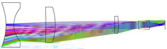
Figure 1.
Optical design of the SW camera. The total axial length equals 85.5 mm. The system consists of three singlet lenses and an achromatic doublet. The aperture stop is situated at the front side of the achromatic doublet. The square detector has a size of 4.92 mm × 4.92 mm. The half FOV is 70°. The sampling of the 12 fields (12 different colors) has been chosen, such that they are separated by the same angle of 6.36°.

Table 1.
Lens data: surface types, materials, thicknesses and diameters. The first and last lens surfaces are aspherical. The first two lenses are made of LAK14 to bend the incoming rays efficiently. The last two lenses form an ahcromatic doublet.
During the optimization process, the effective focal length has been kept constant to 3.3 mm, such that the image height matches the projected full circular object (the Earth) on the detector. Lens thicknesses have been constrained between 2 mm and 5 mm for manufacturing purposes. The total axial length and the maximum diameter of the optical system have been constrained to 9 mm, so that the full camera would fit in 1U. The initial merit function considered the minimization of the RMS spot size. This was adapted to the contrast (or Modulation Transfer Function, MTF) when the spots were reasonably good, i.e., when the spot sizes approximately matched those of the Airy disks. When optimizing the contrast, the spatial frequency has been progressively increased up to 80 cycles/mm, where we expected a good MTF. Near the end of this optimization process, particular attention was paid to the improvement of the manufacturing yield, rather than considering only the best nominal performance. Additionally, finding the best aspheric surfaces has been made possible using the Zemax OpticStudio®’s feature Find Best Asphere tool [15].
In Figure 1, the different colors correspond to the different fields between 0° and 70°. The full FOV is circular and equals 140°. To evaluate the performance of the camera system, we consider the spot diagrams shown in Figure 2. The spot size is simulated for different fields between 0° and 70°, corresponding with the different colors in Figure 1. In Figure 2, the black circles correspond to the Airy disks. When optimizing the optical design, the aim is to match the spot size with the Airy disk, in order to obtain a near-diffraction-limited optical design. Table 2 indicates that the spot sizes approximate the Airy disks for all fields, except for fields 5 and 6, where the spot sizes slightly exceed the Airy disk size, due to a larger amount of aberrations.
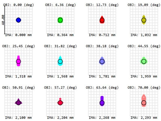
Figure 2.
Spots sizes at = 900 nm, for fields between 0° and 70°. Airy disk radii (black circles) equal 3.192 m. When considering the spots, the system shows a good image quality. OBJ (in degrees) defines the object field and IMA (in mm) defines the image height of the centroid on the detector. The sampling of these 12 fields has been chosen such that they are separated by the same angle.
Table 2.
RMS spots sizes for the different fields in Figure 2. At 900 nm, only the 5th and 6th fields have a spot size exceeding that of the Airy disk.
Regarding the Seidel aberrations, the major contribution comes from distortion (Figure 3). Additionally, it appears that the distortion is mainly induced by the first lens surface, which is aspherical. While this surface enables us to avoid other aberrations, it is the main contributing factor to the distortion. This is because, as stated in Section 2.1, there is no particular requirement on the distortion, since it can be measured during pre-flight characterization, and can be taken into account during the in-flight processing. Among the aberrations that are presented in Figure 3, the dominant aberration is the distortion, which is a common aberration in wide-field imaging systems since this aberration generally increases with the field. Figure 4 gives us a better understanding of the amount of distortion that is present in the optical system. It presents the total distortion (in %), showing that distortion is maximal at 70°, where it equals 74.6%.
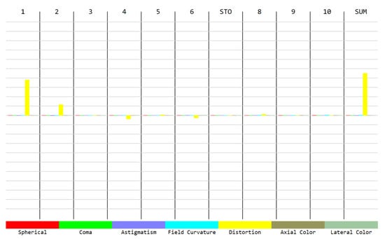
Figure 3.
Five Seidel aberrations and (axial and lateral) chromatic aberrations. The main aberration is the barrel distortion, mainly induced by the first surface. This aberration is illustrated in more detail in Figure 4.
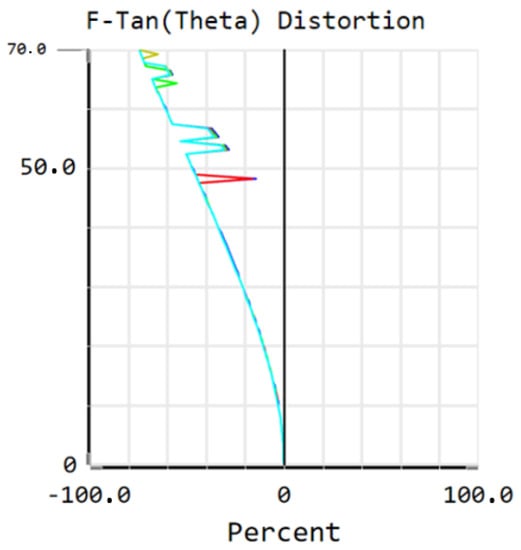
Figure 4.
Barrel distortion is the main aberration present in the optical system, due to the wide field-of-view. Distortion is maximal at 70°, where it equals 74.6%. In this graph, the horizontal axis expresses the distortion in %, and the vertical axis gives the half FOV.
While spots sizes are a good starting point to assess the image quality, we further optimized the Modulation Transfer Function (MTF) quantifying the spatial contrast, resulting in a polychromatic (between 400 nm and 900 nm) diffraction MTF ≥ 0.4 at 78 cycles/mm (Figure 5). This indicates a good performance of the optical design, since the pixel size is 17 m, the MTF should be 0 at 156 cycles/mm.
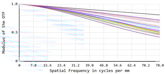
Figure 5.
MTF ≥ 0.4 at 78 cycles/mm. The top black line corresponds to the diffraction limit, and the colors correspond to the different fields, similarly to those presented in Figure 2. Full lines and dashed lines correspond to tangential and sagittal planes, respectively.
3. Simulated Performance of the Instrument
This section focuses on the simulated performance of the instrument. We outline how we intend to use the camera for the measurement of the reflected solar radiation, and we simulate the performance while using the libRadtran [17] radiative transfer software.
3.1. Remote Sensing of Reflected Solar Radiation: Methods
We have not yet experimentally assessed the spectral response of the Aptina MT9T031 detector. However, this spectral response approximates that of a typical R, G, B CMOS sensor. Therefore, and in view of estimating the performance of the SW camera, we constructed synthetic spectral responses that are close to the typical R, G, B CMOS responses as described in [13]. The Red channel has a peak sensitivity just above 600 nm. The Green channel has a primary peak sensitivity near 550 nm and a secondary peak above 800 nm, while the Blue channel has a primary peak sensitivity near 450 nm and a secondary peak above 800 nm, coinciding with the secondary green peak. The following equations reproduce the desired behaviour.
, as described by Equation (1), is the spectral response of the bare CMOS detector without color filter. The spectral responses of the red (), green (), and blue () channel, as described by Equations (2)–(4), respectively, are illustrated in Figure 6.
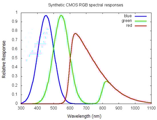
Figure 6.
Synthetic spectral responses of the Red, Green, and Blue components of a CMOS camera. The Red, Green, and Blue channels have peak sensitivities above 600 nm (Red), near 550 nm, and above 800 nm (Green), near 450 nm, and above 800 nm (Blue).
During flight, a vicarious calibration of these channels will be applied by observing deep space and stable Earth targets, such as aerosol free ocean, desert, permanent snow/ice, similar to [18]. This calibration will provide the calibrated spectral radiances , , and .
Next, these calibrated radiances need to be converted into spectral fluxes using empirical spectral Angular Dependency Models (ADMs) , by ways of Equation (5)
where ‘X’ equals ‘R’, ‘G’, or ‘B’. We assume that the ADMs can be derived from a large ensemble of imager data, following a procedure similar to [19].
For the estimation of the RSR, we will use linear regression to calculate the broadband albedo from the narrowband spectral albedos , , , with linear regression parameters (, , , ) dependent on the solar-zenith angle , as given by Equation (6):
where the four regression parameters , , , and are the offset, the red gain, the green gain, and the blue gain, respectively. This linear regression is inspired by the so-called slope-offset method used in the Clouds and the Earth’s Radiant Energy System (CERES) processing [20].
Reference spectral fluxes for specific scene types are simulated with the libRadtran radiative transfer software package [17]. Table 3 summarizes the used reference scene types.
Table 3.
Scene types for radiative transfer simulations.
The simulated spectral fluxes for the scene types ocean, vegetation, desert, and water cloud for a solar-zenith angle of 45° are illustrated in Figure 7. The spectral shape of these radiation fluxes are quite different, with e.g., a peak in the blue region (below 500 nm) for the ocean scene, a peak in the red region (around 700 nm) for the desert scene, and a peak in the near infrared (above 700 nm) for the vegetation scene. These differences, combined with the detector spectral responses of Figure 6, will determine how accurate the broadband albedo can be estimated with Equation (6).
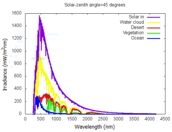
Figure 7.
Simulated outgoing spectral fluxes for a solar-zenith angle of 45° and reference scenes ocean, vegetation, desert and water cloud. Differences between these scenes are notable. The ocean scene has a peak below 500 nm, while the desert scene has a peak around 700 nm and vegetation has a peak above 700 nm.
3.2. Remote Sensing of Reflected Solar Radiation: Results
We performed radiative transfer simulations for the reference scenes listed in Table 3, as introduced in Section 3.1, for 10° solar-zenith angle intervals ranging from 5° to 85°. For every solar-zenith angle , we determine the four regression parameters , , and by a least square fit of Equation (6) for the scene types listed in Table 3. We illustrate the resulting fitted parameters in Figure 8. The offset is nearly zero, the sum of the gains is close to one. The blue gain increases with due to increased Rayleigh scattering at high . The variation of the red gain and the green gain are a consequence of the variation of the blue gain .
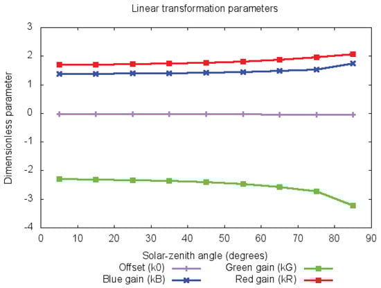
Figure 8.
Spectral fit parameters as function of the solar-zenith angle. The solar-zenith angle ranges from 5° to 85°, in steps of 10°. The offset is nearly zero and the sum of the gains is close to 1. The blue gain increases with due to increased Rayleigh scattering at high and, consequently, induces a variation of the red gain and the green gain .
Using the fitted parameters , , and , the error on the estimate of the broadband albedo , as defined by the Equation (6), is evaluated as a function of the solar-zenith angle , for all scene types of Table 3. The resulting broadband albedo regression error is illustrated in Figure 9. From this figure, we conclude that the broadband albedo error is lower than 3%. This is better than our target, which was a maximal error of 5% [10].
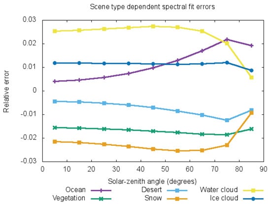
Figure 9.
Scene-type dependent regression error on the broadband albedo as a function of the solar-zenith angle. The relative error on the estimate of the broadband albedo is lower than 3%.
4. Discussion
The state-of-the-art ERB measurements are provided by NASA’s CERES program [7,21]. The spatial resolution for CERES on the Terra and Aqua satellites equals 20 km at nadir. The CERES instrument on-board of TRMM achieved a resolution of 10 km. As TRMM was a precessing satellite, it sampled all viewing angle configurations, which makes it well suited for the development of ADMs [19].
Our optical design of the SW camera shows a sufficiently good image quality to enable scene identification, while featuring broadband estimation by its large bandwidth. The targeted spatial resolution is 2.2 km at nadir, which is achieved for all RMS spots radii that are smaller than 3.2 m over the full FOV. A broader view can be obtained when considering the polychromatic diffraction MTF, which is better to assess the image quality. The performed radiative transfer simulations indicate that, when using the SW camera on a stand-alone basis, the broadband albedo can be estimated with a random error lower than 3% across all simulated scene types and all solar-zenith angles, which is better than the design target of 5% that was put forward in [10]. The next step will be the realization of a prototype of this SW camera. During this step, the detector spectral response should be experimentally determined, and the estimate of the accuracy of the broadband albedo estimate should be updated accordingly.
While conducting a tolerance analysis that accounts for manufacturing imperfections is of major importance before starting the fabrication and assembly of a prototype, we do have confidence in our conceptual design for the following reasons. First, the optical design has only two aspherical surfaces and it uses conventional materials. Second, the optical design was made with the most stringent constraints (largest allowed FOV, smallest allowed F/#, RMS spots radii of the size of one pixel for the largest wavelength). These constraints can still be relaxed. The FOV could be relaxed to e.g., 135°, while the F/# could be relaxed to 4.0 using 650 nm as central wavelength. Depending on the altitude, the FOV can also be relaxed, as long as the camera observes the Earth from limb to limb. In order to allow separating clear-sky and cloudy pixels, the targeted nadir spatial resolution is of the order of 5 km. With a nadir spatial resolution of 2.2 km, our optical design beats this requirement by far.
In addition, it will also be important to perform a full stray-light analysis. Scattering may occur because of the imperfect transmission and surface roughness of optical elements. However, a preliminary analysis has shown that, considering their respective thicknesses, all the considered optical elements have a transmission of more than 90% over the full spectral width, and that this transmission increases to more than 99% starting from 470 nm. The back-reflection will thus be very weak, while an anti-reflection coating can reduce the stray-light even further. Additionally, a path analysis was performed using the non-sequential mode of Zemax OpticStudio®, enabling to study the light transmission through the camera system while taking into account material absorption and light reflection at the lens interfaces. This analysis indicated that almost 97% of the light reaches the detector.
Recently, the Libera mission has been selected by NASA in the framework of the Earth Venture Continuity [9,22]. The mission carries a monochromatic WFOV camera, of which full specifications are currently still unknown. However, in comparison to this camera, which is mainly used for scene identification, our camera also enables a broadband estimation of the shortwave radiation, or reflected solar radiation, owing to its large bandwidth.
We also foresee the development of a LW WFOV camera, targeting the estimation of the thermal radiation [10]. The ensemble of the three WFOV instruments: the radiometer, the SW camera, and the LW camera, will form a compact and relatively low cost payload, suitable for integration on nano- or micro-satellites. Such small satellites can be used to supplement CERES and its follow-on mission Libera, e.g., for improving the sampling of the diurnal cycle. In this context, it is particularly relevant, since currently no follow-on mission for the sampling of the ERB from the morning orbit is foreseen after the end of life of the CERES instrument on the Terra satellite, which is expected around 2026.
5. Conclusions
We proposed to monitor the Earth Radiation Budget with a suite of compact space-based instruments, adequate for the integration within a nano- or micro-satellite. These instruments are a wide field-of-view radiometer, a shortwave camera, and a longwave camera. The core instrument, which was the object of a previous study [10], is a wide field-of-view radiometer aiming to measure the incident solar energy, as well as the Earth’s total outgoing energy, with an accuracy of 0.44 W/m. To supplement this low resolution radiometer, we propose to use wide field-of-view high resolution shortwave and longwave cameras. These cameras will allow:
- separating the shortwave and the longwave radiation;
- increasing the spatial resolution; and,
- performing a scene identification, in particular by discriminating cloudy from clear-sky scenes.
In this paper, we have described our optical design for the wide field-of-view shortwave camera. It consists of three singlet lenses and an achromatic doublet. The full field-of-view equals 140°, enabling to observe the Earth from limb to limb. Using 1536 × 1536 pixels of 3.2 m of the Aptina MT9T031 detector, the nominal spatial resolution equals 2.2 km at nadir, beating the 5 km requirement. Barrel distortion appears to be the main aberration. It is maximal at 70°, where it equals 74.6%. At 900 nm, the optical design is nearly diffraction-limited. A further assessment of the image quality is done by characterizing the polychromatic diffraction Modulation Transfer Function, exceeding 0.4 at 78 cycles per mm. Therefore, we are confident that the wide field-of-view shortwave camera achieves adequate optical performance. The ability to estimate the RSR from the camera spectral measurements was assessed using radiative transfer simulations. Because the precise spectral response of our detector is currently unknown, a synthetic spectral response has been simulated using a classic CMOS RGB response. The incoming and outgoing spectral fluxes have been simulated for different reference scenes using the libRadtran software [17]. Following these radiative transfer simulations, the estimated stand-alone accuracy of the broadband albedo estimate from the SW camera is 3%, which is better than the 5% requirement.
The next steps will include the conceptual design of the WFOV LW camera and the realization of laboratory prototypes of all three instruments.
Author Contributions
L.S. (Luca Schifano) has conducted this study, including methodology, formal analysis and investigation. S.D. has helped with libRadtran. L.S. (Lien Smeesters), S.D. and F.B. have ensured the supervision. S.D. is reponsible for funding acquisition. L.S. (Luca Schifano) has written the original draft. All authors have participated in the review and editing. All authors have read and agreeed to the published version of the manuscript.
Funding
This research was funded by the Solar-Terrestrial Center of Excellence (STCE).
Acknowledgments
B-PHOT acknowledges the Vrije Universiteit Brussel’s Methusalem foundations as well as the Hercules Programme of the Research Foundation Flanders (FWO).
Conflicts of Interest
The authors declare no conflict of interest.
Abbreviations
The following abbreviations are used in this manuscript:
| CERES | Clouds and the Earth’s Radiant Energy System |
| CMOS | Complementary Metal Oxide Semiconductor |
| ERB | Earth Radiation Budget |
| ERBE | Earth Radiation Budget Experiment |
| FOV | Field-Of-View |
| LW | LongWave |
| MTF | Modulation Transfer Function |
| NASA | National Aeronautics and Space Administration |
| OLR | Outgoing Longwave Radiation |
| RAVAN | Radiometer Assessment using Vertically Aligned Nanotubes |
| RMS | Root Mean Square |
| RSR | Reflected Solar Radiation |
| SIMBA | Sun-earth IMBAlance |
| SW | ShortWave |
| TOA | Top-Of-Atmosphere |
| TSI | Total Solar Irradiance |
| WFOV | Wide Field-Of-View |
References
- Dewitte, S.; Clerbaux, N. Measurement of the Earth Radiation Budget at the Top of the Atmosphere—A Review. Remote Sens. 2017, 9, 1143. [Google Scholar] [CrossRef]
- Hansen, J.; Sato, M.; Kharecha, P.; von Schuckmann, K. Earth’s energy imbalance and implications. Atmos. Chem. Phys. 2011, 11, 13421–13449. [Google Scholar] [CrossRef]
- Trenberth, K.E.; Fasullo, J.T.; von Schuckmann, K.; Cheng, L. Insights into Earth’s Energy Imbalance from Multiple Sources. J. Clim. 2016, 29, 7495–7505. [Google Scholar] [CrossRef]
- Von Schuckmann, K.; Palmer, M.D.; Trenberth, K.E.; Cazenave, A.; Chambers, D.; Champollion, N.; Hansen, J.; Josey, S.A.; Loeb, N.; Mathieu, P.-P.; et al. An imperative to monitor Earth’s energy imbalance. Nat. Clim Chang. 2016, 6, 138–144. [Google Scholar] [CrossRef]
- Smith, G.L.; Gibson, G.G.; Harrison, E.F. History of earth radiation budget at Langley Research Center. Available online: https://ams.confex.com/ams/pdfpapers/158948.pdf (accessed on 20 June 2020).
- Barkstrom, B.R. The Earth Radiation Budget Experiment (ERBE). BAMS 1984, 65, 1170–1185. [Google Scholar] [CrossRef]
- Wielicki, B.A.; Barkstrom, B.R.; Harrison, E.F.; Lee, R.B., III; Smith, G.L.; Cooper, J.E. Clouds and the Earth’s Radiant Energy System (CERES): An Earth observing system experiment. Bull. Am. Meteorol. Soc. 1996, 77, 853–868. [Google Scholar] [CrossRef]
- Wong, T.; Smith, G.L.; Kato, S.; Loeb, N.G.; Kopp, G.; Shrestha, A.K. On the Lessons Learned From the Operations of the ERBE Nonscanner Instrument in Space and the Production of the Nonscanner TOA Radiation Budget Data Set. IEEE Trans. Geosci. Remote. Sens. 2018, 56, 5936–5947. [Google Scholar] [CrossRef]
- Earth Venture Continuity Radiation Budget Science Working Group. Measurement and Instrument Requirement Recommendations for an Earth Venture Continuity Earth Radiation Budget Instrument. 2018. Available online: https://smd-prod.s3.amazonaws.com/science-pink/s3fs-public/atoms/files/ERB_SWG_Rept_Draft_07242018_TAGGED.pdf (accessed on 14 May 2020).
- Schifano, L.; Smeesters, L.; Geernaert, T.; Berghmans, F.; Dewitte, S. Design and analysis of a next generation wide field-of-view Earth Radiation Budget radiometer. Remote. Sens. 2020, 12, 425. [Google Scholar] [CrossRef]
- Dewitte, S.; Nevens, S. The Total Solar Irradiance Climate Data Record. Astrophys. J. 2016, 830, 25. [Google Scholar] [CrossRef]
- Ackerman, S.A.; Holz, R.E.; Frey, R. Cloud Detection with MODIS. Part II: Validation. Am. Meteorol. Soc. 2008, 25, 1073–1086. [Google Scholar]
- Skorka, O.; Kane, P.; Ispasoiu, R. Color correction for RGB sensors with dual-band filters for in-cabin imaging applications. In Proceedings of the Autonomous Vehicles and Machines Conference 2019, Burlingame, CA, USA, 13–17 January 2019; Society for Imaging Science and Technology: Springfield, VA, USA, 2019; pp. 46-1–46-8. [Google Scholar]
- Pérez, L.L.; Walker, R. GOMX-4—The twin European mission for IOD purposes. In Proceedings of the 32nd Annual AIAA/USU Conference on Small Satellites, Logan, UT, USA, 4–9 August 2018. [Google Scholar]
- Normanshire, C. Designing for As-Built Performance with High-Yield Optimization. Zemax Knowledgebase, KA-01837. Available online: https://my.zemax.com/en-US/Knowledge-Base/kb-article/?ka=KA-01837 (accessed on 12 May 2020).
- SCHOTT® Website. Available online: https://www.schott.com/ (accessed on 12 May 2020).
- Mayer, B.; Emde, C.; Buras-Schnell, R.; Kylling, A. Radiative transfer: Methods and applications. In Atmospheric Physics; Springer: Berlin/Heidelberg, Germany, 2012; pp. 401–415. [Google Scholar]
- Decoster, I.; Clerbaux, N.; Baudrez, E.; Dewitte, S.; Ipe, A.; Nevens, S.; Blazquez, A.; Cornelis, J. Spectral Aging Model Applied to Meteosat First Generation Visible Band. Remote Sens. 2014, 6, 2534–2571. [Google Scholar] [CrossRef]
- Loeb, N.; Smith, N.M.; Kato, S.; Miller, W.F.; Gupta, S.K.; Minnis, P.; Wielicki, B. Angular Distribution Models for TOA radiative flux estimation from the CERES instrument on the TRMM satellite. Part 1: Methodology. J. Appl. Meteorol. 2002, 42, 240–265. [Google Scholar] [CrossRef]
- Loeb, N.G.; Priestley, K.J.; Kratz, D.P.; Geier, E.B.; Green, R.N.; Wielicki, B.A.; Hinton, P.O.R.; Nolan, S.K. Determination of Unfiltered Radiances from the Clouds and the Earth’s Radiant Energy System Instrument. J. Appl. Meteorol. 2000, 40, 822. [Google Scholar] [CrossRef]
- Loeb, N.G.; Doelling, D.R. Clouds and the earth’s radiant energy system (CERES) energy balanced and filled (EBAF) top-of-atmosphere (TOA) edition-4.0 data product. J. Clim. 2018, 31, 895–918. [Google Scholar] [CrossRef]
- Pilewskie, P. Libera and Continuity of the ERB Climate Data Record. CERES STM 2020, Virtual Meeting. Available online: https://ceres.larc.nasa.gov/documents/STM/2020-04/27_CERES_Science_Team_Meeting_pilewskie_29apr20_12PM.pdf (accessed on 20 June 2020).
© 2020 by the authors. Licensee MDPI, Basel, Switzerland. This article is an open access article distributed under the terms and conditions of the Creative Commons Attribution (CC BY) license (http://creativecommons.org/licenses/by/4.0/).