Global Assessments of the HY-2B Measurements and Cross-Calibrations with Jason-3

Abstract

The HY-2B satellite was successfully launched on 25 October 2018. One of the main payloads of the HY-2B was a radar altimeter. In the present study, the quality of the HY-2B along-track sea surface heights (SSH), significant wave heights (SWH), and sea surface wind speeds (SSWS) were assessed, including their precision and accuracy. In order to achieve this goal, the mono-mission metrics of the HY-2B were analyzed and compared with those of the Jason-2 and Jason-3 over the same periods of time. The results of both direct comparison and cross comparison methods were presented in this study. The comparison results indicated that the quality of the HY-2B satellite’s geophysical data records (GDRs) data was excellent, with 95% of the sea surfaces effectively observed between 82 degrees north and south latitudes. In addition, the standard deviation of the sea level anomalies (SLA) at the single mission crossovers was 4.6 cm to 5.8 cm, and at the dual-crossovers with Jason-3, the standard deviation was determined to be 5.1 cm to 5.8 cm. The accuracy levels of the significant wave heights and products of the HY-2B satellite radar altimeter were observed to be greater than 0.3 m and 1.4 m/s (STD), respectively. Therefore, it was concluded in this study that the data quality and system performance of the HY-2B satellite were excellent and stable, and could be widely utilized in such fields as global sea-level change monitoring, wave numerical assimilation predictions etc.

1. Introduction

The HY-2B (Haiyang-2B) satellite is the second marine dynamic environment satellite launched by China, the first being the HY-2A satellite. It is equipped with a dual-frequency radar altimeter (Ku and C bands), a microwave scatterometer, a microwave radiometer, a calibration microwave radiometer designed for altimeter wet troposphere corrections, a data collection system and an automatic identification system.

Since its launch on 24 November 2018, the HY-2B satellite has been providing oceanic, atmospheric, and ice measurements [1]. In the future, the HY-2B satellite will form a constellation with the HY-2C and HY-2D marine dynamic environment satellites to be launched in the near future. The frozen elliptical orbit of the HY-2B satellite is sun-synchronous with a 14-day period for ocean observations during the early lifetime of the satellite, and 168-day period for geodetic applications in the end of the lifetime.

As part of the HY-2B mission, a two-frequency radar altimeter for achieving measuring ranges with accurate ionospheric corrections was introduced. The two-frequency radar altimeter operates at 13.58 GHz (Ku-band) and 5.25 GHz (C-band). The main design parameters of HY-2B radar altimeter are given in

Table 1. Main parameters of the HY-2B radar altimeter.

Frequency	13.58 GHz (Ku), 5.25 GHz (C)
Pulse-limited footprint	<2 km
Frequency bandwidth	320 MHz, 80 MHz, 20 MHz adaptive
Pulse repetition frequency	2.3 kHz (Ku), 0.76 kHz (C)
Pulse-width	3.125 ns
Antenna aperture	1323 mm ± 10 mm
Antenna beamwidth (3dB)	1.2° ± 0.1° (Ku), 3.2° ± 0.3° kHz (C)

.

In order to accurately measure the distances from the satellite to the sea surfaces while avoiding the effects of drifts caused by the ageing of the device [2,3,4,5], the HY-2B satellite carries a rubidium atomic clock and a Global Positioning System (GPS) second pulse design to ensure that the timing remains accurate between and within one second. At the same time, in order to improve the accuracy of the distance measurements, the HY-2B’s radar altimeter has been modified as a vertical surface direction (nadir-looking) device. However, in the HY-2A satellite, the radar altimeter continues to point to the center of the Earth.

Unlike the HY-2A and the Jason-1/2/3 satellites, which use Doris to precisely determine their orbits, the HY-2B is not equipped with a Doris system. The HY-2B satellite instead adopted dual frequency GPS for its precise orbital determinations.

When compared with interferometric radar altimeters (such as SWOT), the radar altimeter of the HY-2B satellite is a typical traditional radar altimeter. The HY-2B satellite radar altimeter can be used to derive sea surface heights, significant wave heights, sea surface wind speeds, gravity field, ocean circulations, etc.

Calibration and validation processes are very important and indispensable components of every satellite altimetry system [6]. Accurate and objective calibrations and validations not only provide reliable information for the users of the data products, but also provide support and assistance for improving the accuracy of the data products. Therefore, accurate calibrations between different satellite missions, as well as careful monitoring of mission execution results over time, are also crucial to ensuring the continuity of historical satellite altimeter records and allowing accurate climate research to be conducted.

This study focused on the long-term monitoring of the HY-2B altimetry system using data from all of the available GDR products so far (cycles 1 to 36, the latest data in cycle 36 is less than one cycle), which accounted for more than 16 months worth of data. This included careful assessments of all the altimeter parameters, performance assessments, and cross-calibrations with Jason-3 measurements.

Although the HY-2B satellite radar altimeter is a dual frequency altimeter, the C-band was mainly designed to solve the delay corrections of the ionospheric paths. In all of the other cases, the measurement results of the Ku band were consistently used. Therefore, only the measurement results of the Ku band were evaluated in this study.

In Section 2 of this study, the HY-2B data to be evaluated, along with the Jason-3 products used for the assessments, are introduced. Section 3 mainly presents the observation data which were provided by the HY-2B satellite, and this study’s comparison results with the Jason-3 data. Section 4 mainly discusses the comparison and analysis results of the observational noise of the HY-2B satellite. Section 5 details the evaluations of the inversion parameters, such as the mispointing angles, backscatter coefficients, sea surface wind speeds, significant wave heights, and sea state bias, etc. In Section 6, the accuracy of height measurement products of the HY-2B satellite, such as the SSH and SLA, are analyzed, and this study’s conclusions are presented.

2. Experimental Data and Assessment Methods

2.1. HY-2B Satellite Radar Altimeter Products

The level-2 products of the HY-2B satellite radar altimeter include three GDR (Geophysical Data Records) series. The first series is OGDR (Operational Geophysical Data Record), which mainly provide near real-time significant wave heights and sea surface wind speeds data to meteorological users. In addition, OGDR is designed to provide altimeter range, geophysical corrections together with a real-time finite precision orbit. OGDRs are available with latency of about 3 h. The second series is IGDR (Interim Deophysical Data Record), which mainly provides the sea surface height products to operational oceanography users with a more accurate orbit. IGDR also include significant wave heights and sea surface wind speeds. IGDRs are available with a latency of 2 days. The third series is the GDR product, which is calibrated and fully validated. GDRs are available with a latency of 24 days.

The current product version of HY-2B adopts a maximum likelihood estimator of the four variables of interest [7]. In other words, the standard ocean maximum likelihood estimator (MLE4) was used to retrieves the 4 parameters that can be inverted from the altimeter waveforms: altimeter range, significant wave heights (SWH), Sig0, and square of mispointing angle. In addition to the MLE4 retracking parameters, MLE3 retracker parameters are also included in the HY-2B OGDR, IGDR, and GDR products. The HY-2B data used in this study are from retracking each 20 Hz waveform independently, and, as for Jason-3, there is no along-track filtering.

In this study, the GDR products of the HY-2B satellite radar altimeter from 30 October 2018 to 12 March 2020 were used. These data products were obtained through the data distribution system of the National Satellite Ocean Application Service (https://osdds.nsoas.org.cn/). The standard GDR products included the 20 Hz and 1 Hz significant wave heights, backscatter coefficients, distance measurements, etc. as required by this study. At the same time, it also included the corrections for the different types of height measurement errors.

2.2. Jason-2/3 Satellite Radar Altimeter Products

In order to compare and evaluate the accuracy of the HY-2B satellite radar altimeter data products, the Jason-2/3 level 2 GDR data were selected for comparison purpose in this study. The reasons for choosing Jason-2/3 data products included the following aspects: 1. The Jason-2/3 satellite radar altimeters were the follow-up satellites of TOPEX/Poseidon and Jason-1. After nearly 30 years of development, the measurement accuracy of this series of satellites have been determined to be high; 2. The Jason-2/3 satellite radar altimeters data products have been calibrated and evaluated using on-site and similar satellites; 3. The lifetime of HY-2B was included by the lifetime of the Jason-3, and also overlapped with that of the Jason-2 satellite radar altimeter at the end of Jason-2′s lifetime; 4. There were many crossovers between the Jason-3 satellite’s ground track and that of the HY-2B satellite.

In this study, the Jason-3 data selected to evaluate the HY-2B data product were the level 2 GDR data from 30 October 2018 to 5 January 2020 (the latest GDR data product available in this study). Also, the Jason-2 product was from 30 October 2018 to 27 February 2019. The observational results of the HY-2B satellite radar altimeter was comprehensively evaluated using the Jason-3 data. The Jason-2 data were only used to test the observational noise and SLA power spectrum of the HY-2B satellite.

2.3. Experimental Method

In the various assessments performed in the present study, different methods were adopted. For the observational noise, in this study’s assessments of the data availability and SLA power spectral density of the satellite radar altimeter were included the advantages and disadvantages of each measurement, which were analyzed using direct comparisons.

The sea surface heights, backscatter coefficients, and significant wave heights were mainly evaluated using cross-comparison methods. The cross-comparisons consisted of the mono-mission crossovers of the ascending and descending orbits, and multi mission crossovers of the ground tracks. The mono-mission crossovers of the ascending and descending orbits were mainly used to evaluate the accuracy of the sea surface height products.

When two satellite altimeters were in orbit at the same time, the more accurate altimeter data could be used as references to evaluate the data quality of the other satellites. The method used was the multi-mission cross-calibration assessment. This type of method is widely used to evaluate newly launched satellite radar altimeter data products using calibrated satellite radar altimeter data [8,9,10,11,12,13,14,15,16].

Only the Jason-3 data were used when evaluating the HY-2B data products by the adopted cross-calibration assessment method. Jason-3 is the follow-up satellite of T/P, Jason-1 and Jason-2. Due to the fact that the data products have been calibrated with high accuracy, the products can be used as references for other altimeter satellite missions. In this study, the sea surface height data obtained from the Jason-3 satellite when in orbit at the same time as the HY-2B satellite were used to analyze the differences in the significant wave heights, backscatter coefficients, sea surface heights, and sea level anomalies at the crossover points of the two satellites. Then, the accuracy of the sea surface height data of the HY-2B satellite was evaluated.

There are many methods available to select crossover data, such as the nearest observation point; nearest point averaging; nearest observation point interpolation method, et al. Each method has been found to have its advantages and disadvantages. The method selected in this study was the near observation point interpolation method [16] used by Jiang et al. This method avoided the inaccurate or wrong assessments caused by the inaccurate positioning measurements at the crossovers. In this study, the mean and standard deviation distributions of the sea surface heights and their differences were mainly analyzed, as well as sea-level anomalies and their observed differences at the crossover points.

3. Data Availability

The data availability statistics method adopted in this study utilized such information as the surface type, precise orbit determination, and range data in HY-2B standard products, along with the data corrections. The surface types were DEM (digital elevation model) data using ETOPO1 (1 arc-minute global Earth’s Topography). The precise orbit determination was calculated based on the dual frequency GPS mounted on the HY-2B satellite.

Then, in order to compare and analyze the data availability of the level 2 products of the HY-2B radar altimeter, the same method was used in this study to analyze the Level 2 products of the Jason-3 during the same timeframes.

There were three cases for discussion in this study. The first was the selection of all sea area data, including the polar areas, in which only the HY-2B data were analyzed. The second was the selection of the data between the southern latitude of 66° and the northern latitude of 66°, which were consistent with the Jason-3 measurement range. Finally, the data which showed that the latitude is lower than 50° were selected in order to minimize the impacts of the land and sea ice on the data availability analysis results.

Since the availability of the Level 2 product data of the HY-2B and Jason-3 satellites was determined to be approximately 90%, this study used the data missing rate to explain the obtained results in order to be clearer and more intuitive.

However, it was also necessary to consider the influences of the inversions of single event upsets since the HY-2B satellite had experienced six inversions of single event upsets over South America since its launch. Due to the fact that the satellite’s altimeter had not reset immediately after the inversions of single event upsets, the data between the single events upset events and the next reset were lost.

Table 2. The time of single event upset event HY-2B satellite has experienced.

	Time (UTC)
1st	2019/06/14 11:06–2019/06/15 00:10
2nd	2019/08/17 10:18–2019/08/17 23:40
3rd	2019/08/26 10:54–2019/08/28 06:40
4th	2019/12/13 01:50–2019/12/13 13:24
5th	2019/12/16 07:03–2019/12/16 11:07
6th	2020/02/26 09:10–2020/02/27 00:28

shows the times of each single event upset event. However, the lost data were not within the analysis scope of this study’s data available experiment. That is to say, only the level 2 products under normal observations were statistically analyzed.

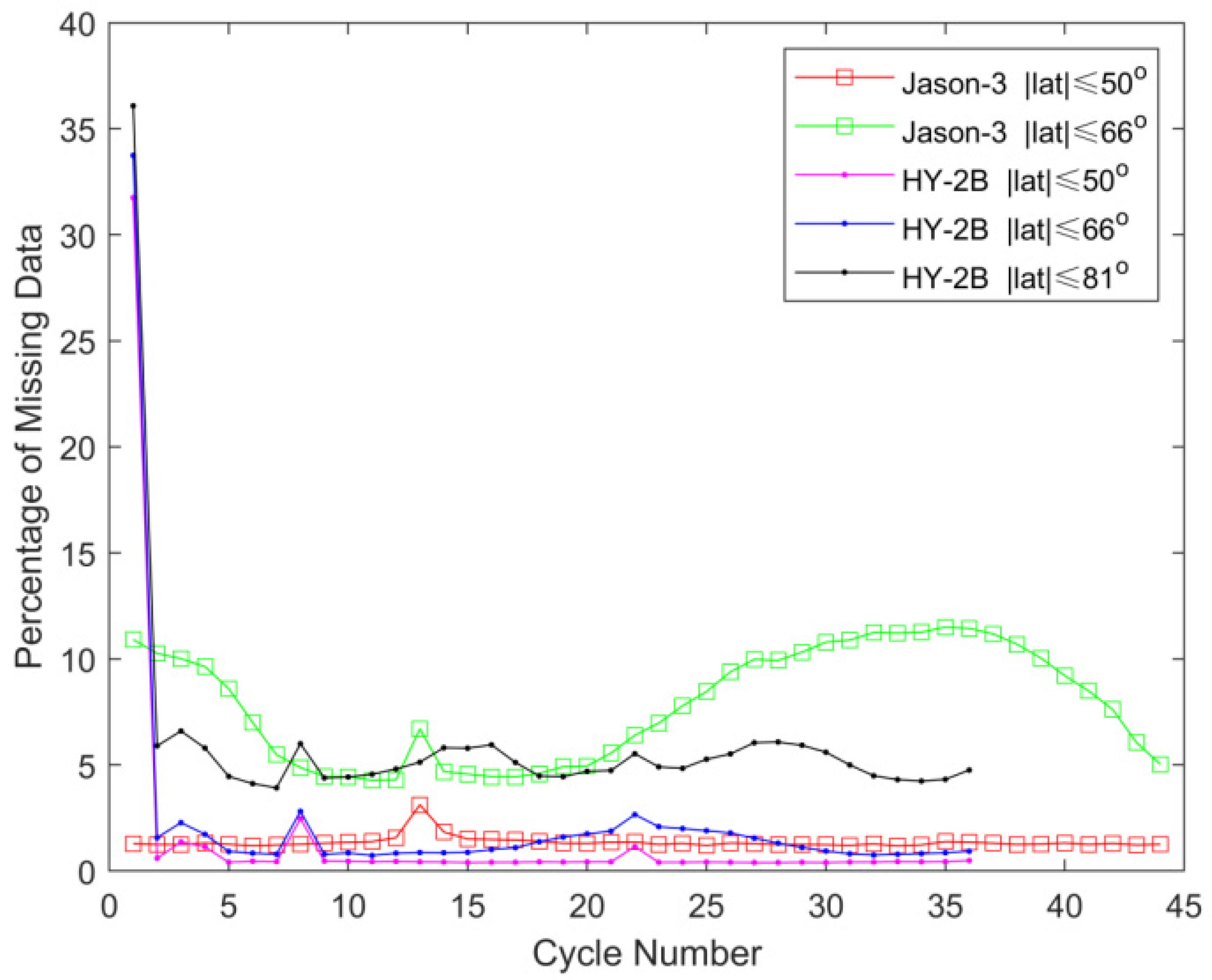
In this research study, missing measurements were calculated by comparison to theoretical orbit ground pattern using the DEM. The data missing rates of the HY-2B and Jason-3 satellites were calculated applying the same procedure. If the DEM is ocean and the data quality flags are land, the observation point is considered unavailable. In the statistical results, the rates were divided into different ranges of latitude. The highest latitude of the HY-2B observations was approximately 80°. Therefore, the missing rates of all the observation data were calculated in this study. Then, in order to make a direct comparison with the Jason-3 satellite, the data missing rates in the range of |latitude| ≤66° and |latitude| ≤50° were also calculated.

The following diagram, Figure 1 shows this study’s comparison results of the data missing rates of the HY-2B and Jason-3 satellites in different latitudes. As the first cycle was still within the orbital adjustment and load adjustment phases of the satellite, the data missing rates of the HY-2B satellite radar altimeter during the first cycle were relatively large. The data missing rates of the global statistics reached 36.08%, and the data missing rates of |latitude| ≤66° and |latitude| ≤50° were 33.74% and 31.75%, respectively. However, with the exception of the first cycle, the data missing rates of HY-2B in all of the observation areas were approximately 5%, and the data missing rates within the range of |latitude| ≤66° and |latitude| ≤50° were determined to be 1.31% and 0.56%, respectively.

In addition, using the same statistical method as in the |latitude| ≤66° and |latitude| ≤50° areas, the data missing rates of the Jason-3 satellite were determined to be 7.59% and 1.38%, respectively.

Clearly, the data availability of the HY-2B satellite was significantly higher than that of the Jason-3 satellite.

In summary, due to the fact that the HY-2B satellite had 386 passes in a cycle and Jason-3 satellite had only 254 passes in a cycle, the number of data cycles of the Jason-3 satellite was larger than that of the HY-2B satellite during the same time period.

4. Noise Measurements

The data of the 3rd and 4th cycles of the HY-2B satellite (26 November to 24 December of 2018) were used in this study for the statistical analysis process. The selected data of the Jason-3 satellite’s altimeter were within the same period as those of the HY-2B satellite, and the data screening criteria were as follows:

(1)

The latitude was less than ±50°;

(2)

There were at least 19 valid data within a one second period;

(3)

The surface type was ocean.

As an indicator for the precision of a parameter at 1 Hz, the standard deviation (std) of this parameter over 20 consecutive 20 Hz measurements is considered and those as a function of significant wave height is evaluated. The median of the standard deviations for each observation is calculated to obtain the performance curve.

4.1. Noise Levels of the Ranges

In the present study, the range referred to the distance from the satellite to the sea surface measured by the satellite’s radar altimeters, which was obtained by the tracking distances on the satellite plus the re-tracking correction values and the instrument error corrections. In order to determine the 1 Hz range from the 20 Hz range data, it was necessary to conduct linear regression of twenty 20 Hz range measurement values in one second to achieve a straight line by fitting. According to the fitting results, the standard deviation of the 20 Hz range data in one-second intervals was calculated, and its value reflected the noise level of the 20 Hz range. It was determined that if the 20 measurements were regarded as uncorrelated, then the noise level of the 1 Hz range could be obtained by dividing the standard deviation by $\sqrt{20}$.

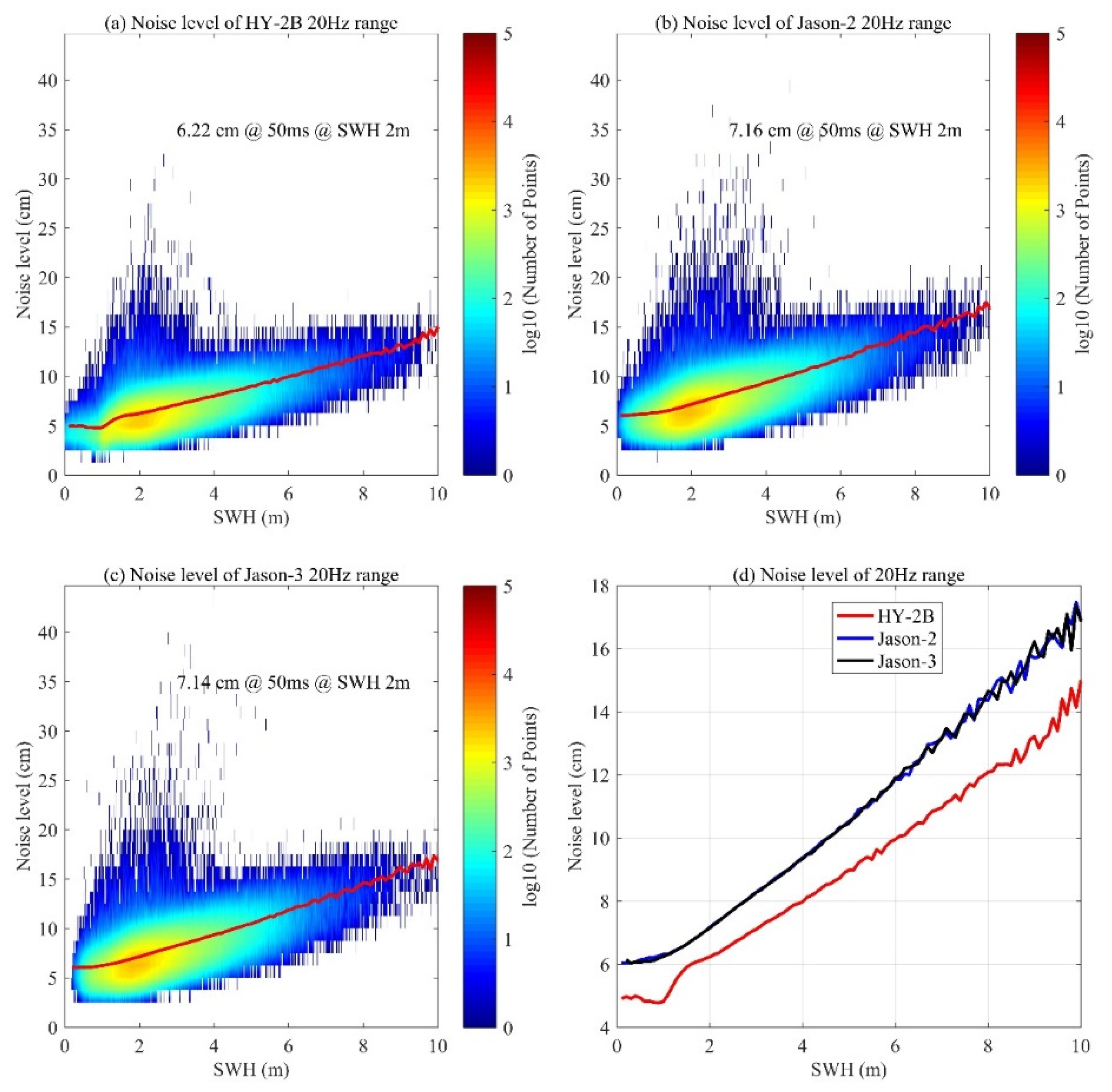
Figure 2 and Figure 3 show the statistical data of the noise levels in the ranges of the 20 Hz and 1 Hz Ku bands, respectively. In the Figure 2 and Figure 3, (a), (b), and (c) represent the scatter diagrams of the noise levels and significant wave heights SWH of the HY-2B, Jason-2, and Jason-3 satellites, respectively. In addition, and the red curves in the Figure 2 and Figure 3 indicate the median of the standard bias calculated according to the significant wave height. For the convenience of comparison, the red curves from Figure 2a–c and Figure 3a–c are displayed in the Figure 2d and Figure 3d. The noise levels of the various ranges had increased with the increases in the significant wave heights SWH, and the noise levels of the ranges obtained by the HY-2B satellite were lower than those obtained by the Jason-2 and Jason-3 satellites in all of the significant wave height ranges. For example, under the conditions of 2 m significant wave heights, the noise levels of the HY-2B altimeter in 20 Hz Ku band range was 6.22 cm. Meanwhile, the Jason-2 and Jason-3 satellites were determined to be 7.16 cm and 7.14 cm, respectively. Furthermore, the noise level of the corresponding HY-2B altimeter in 1 Hz Ku band range was 1.39 cm, while those of the Jason-2 and Jason-3 were 1.60 cm and 1.59 cm, respectively.

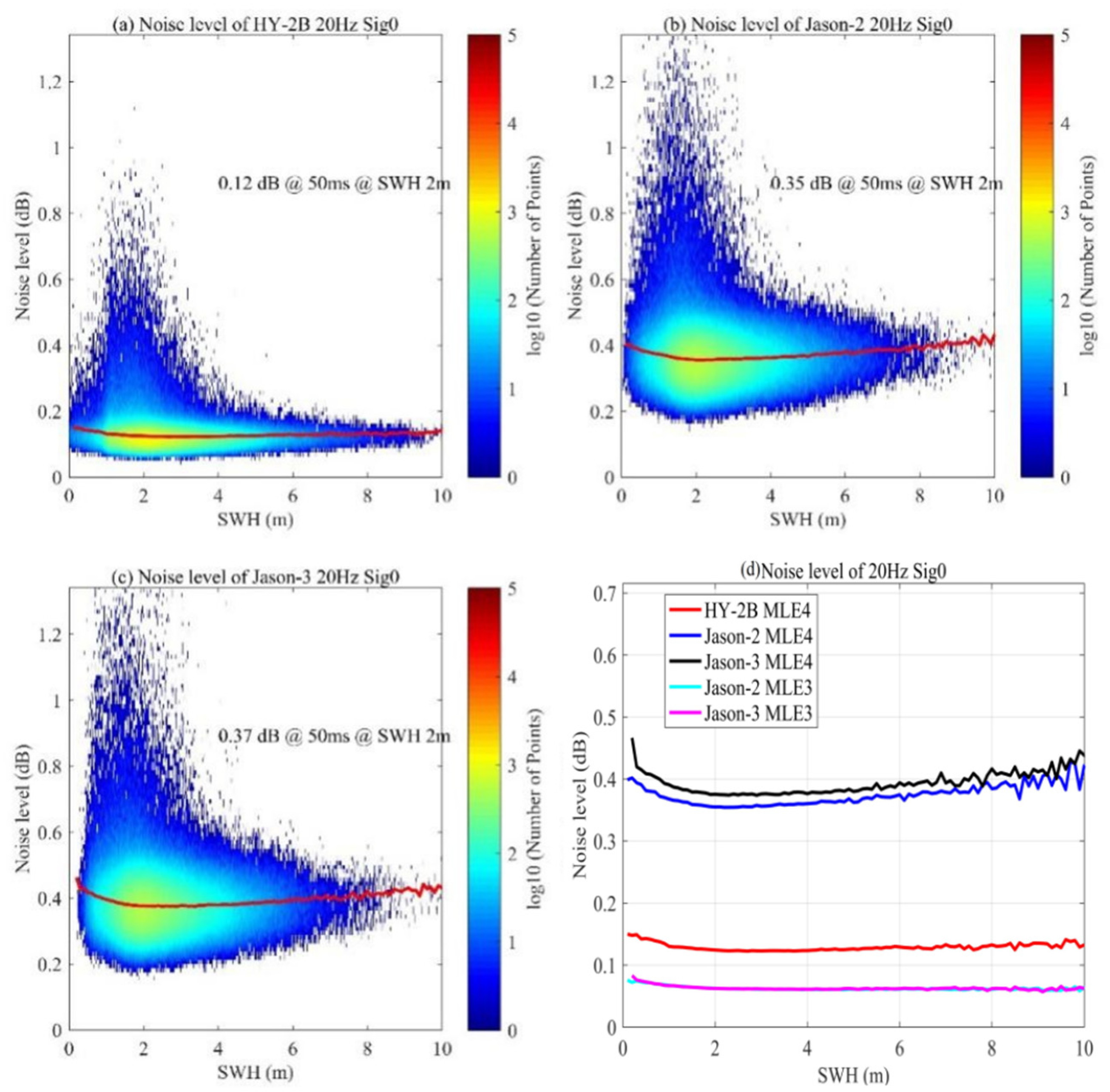
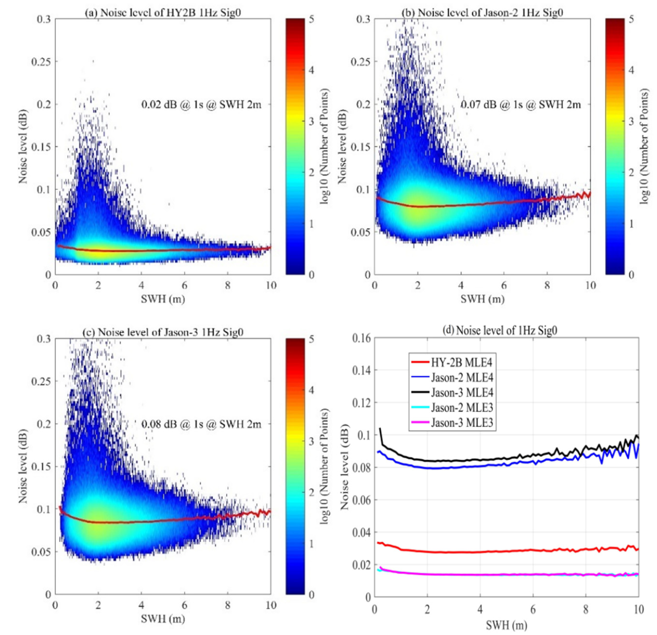
4.2. Noise Levels of the Backscatter Coefficients

The echo amplitudes can be obtained by retracking the echo waveforms of the altimeters using the MLE4. Subsequently, the backscatter coefficients can be determined. The 1 Hz backscatter coefficients along the orbits can be obtained by averaging the 20 Hz backscatter coefficients. In the present study, the standard deviation of twenty 20 Hz backscatter coefficient measurement values within one second intervals was calculated, which reflected the noise levels of the 20 Hz backscatter coefficients. The 20 Hz backscatter coefficient measurement values within one second were regarded as unrelated to each other. Therefore, the noise levels of the 1 Hz backscatter coefficients could be determined by dividing the standard deviation obtained by $\sqrt{20}$.

Figure 4 and Figure 5 detail the statistical data of the noise levels of the backscatter coefficients in the 20 Hz and 1 Hz Ku bands, respectively. In the Figure 4 and Figure 5, (a), (b), and (c) represent the scatter diagrams of the noise levels of backscatter coefficients of the HY-2B, Jason-2, and Jason-3 satellites, respectively, and the red curves in the Figure 4 and Figure 5 indicate the median of the standard deviation calculated according to the significant wave height. The red curves in Figure 4a–c and Figure 5a–c are displayed in the same figure (d). It can be seen from the figure that the noise levels of the backscatter coefficients had increased with the increases in the significant wave heights when the significant wave heights were larger than 2 m. In addition, the noise levels of backscatter coefficients obtained by the HY-2B satellite were lower than those obtained by the Jason-2 and Jason-3 satellites in all of the significant wave height. Furthermore, under the conditions of 2 m significant wave heights, the noise level of the backscatter coefficients of the HY-2B satellite’s altimeter in the 20 Hz Ku band was determined to be 0.12 dB, while that of the Jason-2 and Jason-3 satellites were 0.35 dB and 0.37 dB, respectively. It was also determined that the noise level of the backscatter coefficients of the corresponding HY-2B satellite’s altimeter in the 1 Hz Ku band was 0.02 dB. Meanwhile, those of the Jason-2 and Jason-3 satellites’ were 0.07 dB and 0.08 dB, respectively.

However, the Sig0 obtained by using MLE-3 retracking algorithm after empirical correction is significantly better than that of using standard MLE-4 [17]. The Sig0 noise of Jason-2 and Jason-3 after empirical correction is also better than that of HY-2B.

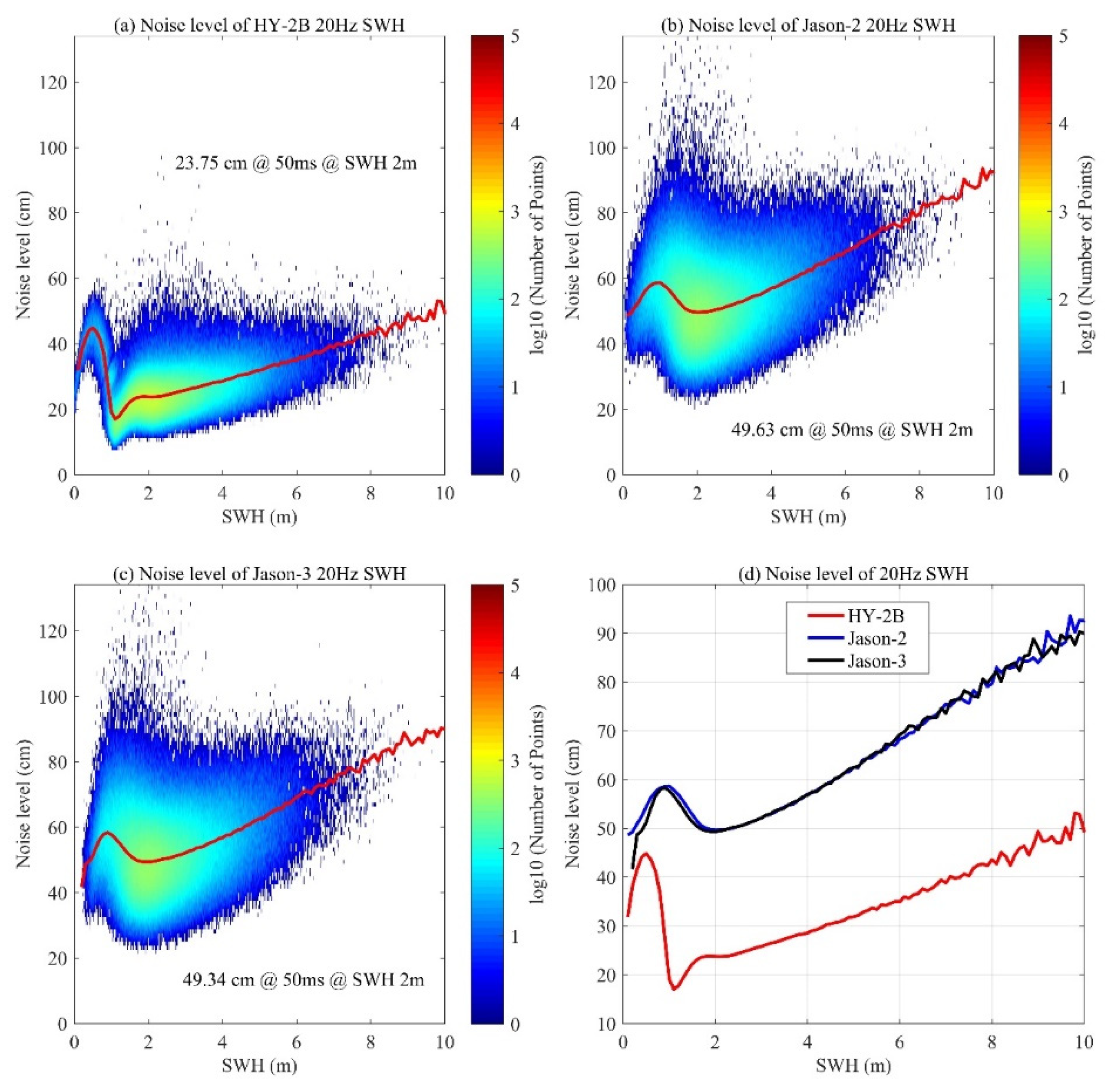
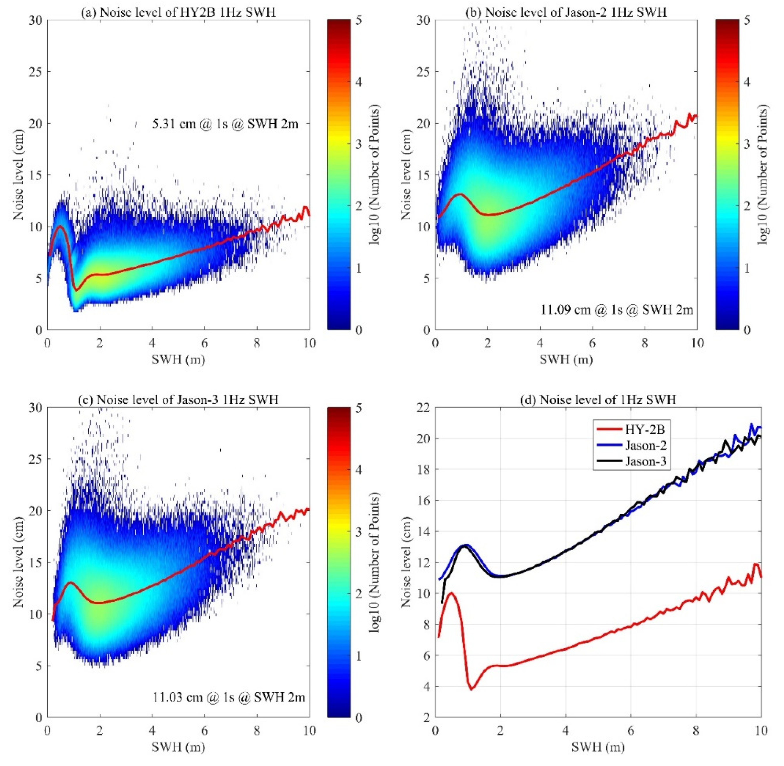
4.3. Noise Level of the Significant Wave Height

The significant wave height can be obtained by re-tracking the echo waveform of the altimeter. The significant wave height of 1 Hz along the track is obtained by averaging the significant wave height of 20 Hz. The standard deviation of 20 significant wave height measurements within 1 s is calculated, which reflects the noise level of the significant wave height of 20 Hz. The 20 significant wave height measurements within 1s are regarded as uncorrelated, and the standard deviation obtained can be divided by $\sqrt{20}$ to reflect the 1 Hz noise level of the significant wave height.

Figure 6 and Figure 7 show the statistics of the noise level of the significant wave height in the 20 Hz and 1 Hz Ku bands respectively. (a), (b) and (c) in the Figure 6 and Figure 7 respectively represent the scatter diagrams of HY-2B, Jason-2 and Jason-3′s noise levels. The red curves in the subfigure a-c are the median of the standard deviation calculated according to the significant wave height information in the step of 0.1m. Subfigure (d) shows the corresponding red curve in subfigures (a), (b) and (c) in the same figure in Figure 6 and Figure 7. It can be seen from each subfigure (d) that when the significant wave height is greater than 2 m, the noise will increase with the increase of the significant wave height, and the noise level of the significant wave height obtained by HY-2B is lower than Jason-2 and Jason-3. Under the condition of 2 m significant wave height, the noise level of the HY-2B altimeter in the 20 Hz Ku band is 23.75 cm, while those of Jason-2 and Jason-3 are 49.63 cm and 49.34 cm, respectively; the noise level of the corresponding HY-2B altimeter in the 1 Hz Ku band is 5.31 cm, and those of Jason-2 and Jason-3 are 11.09 cm and 11.03 cm respectively.

There are two reasons why HY-2B range noise level is better than one from Jason-3. One is that the measurement noise of HY-2B instrument is better than that of Jason-3. The other is data processing. More detailed research and comparison to confirm the reasons.

5. Analysis of the Altimeter Parameters

In the next section, this study presents the assessments of re-tracked parameters. These assessments allowed for the highlighting of any unusual events encountered by the HY-2B satellite’s altimeter during the study period. It should be noted that the altimetric distance assessments were as described in the following section (sea level performances).

5.1. Squared Mispointing from the Waveforms

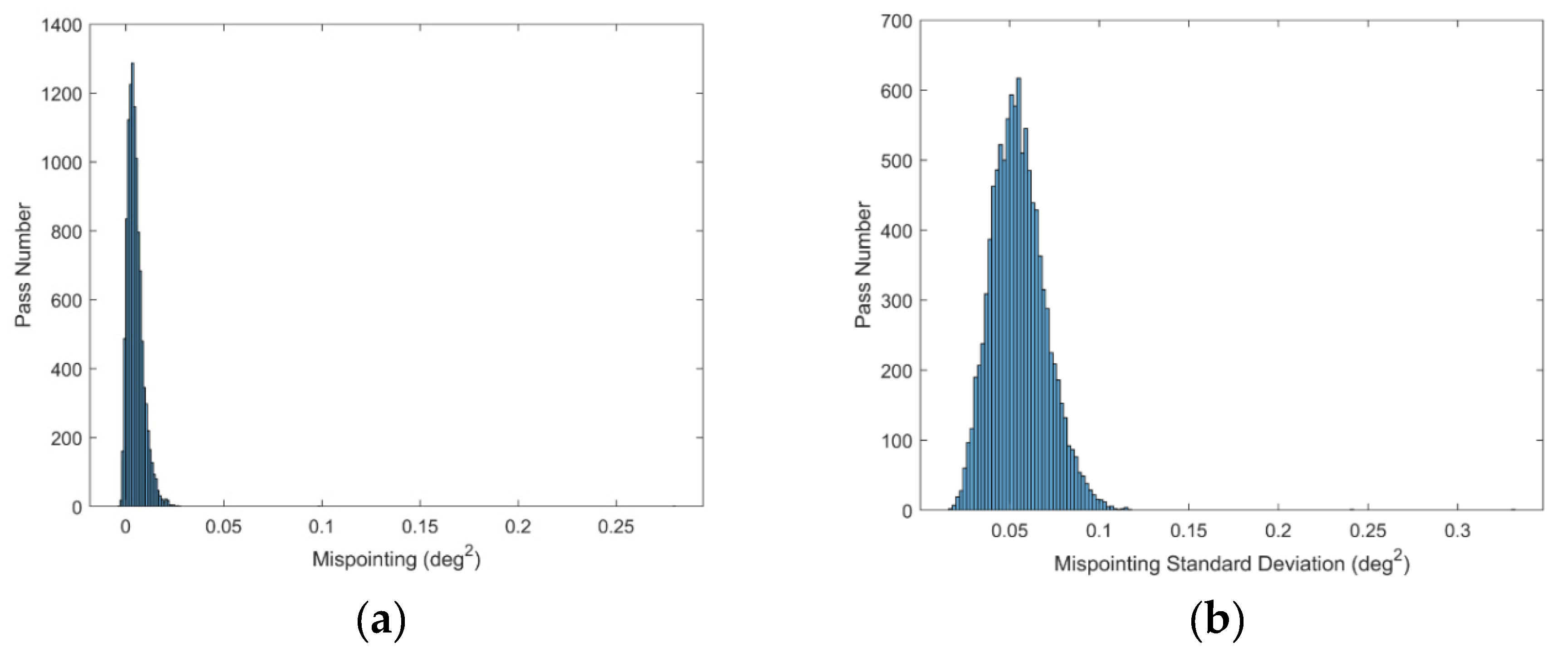
During the measurement processes of the satellite radar altimeter, the mispointing angles of the antenna have significant impacts on the echo waveforms of radar altimeter. Therefore, major impacts on the measurement results of sea surface height may be encountered. The HY-2B satellite’s radar altimeter is a high-resolution radar device with nadir pointing and a pulse limit system. Mispointing angles are one of the parameters which can be retraced and estimated from the echo waveforms of the altimeter. In order to achieve the purpose of Cal/Val, this study calculated and monitored the average pass values of the mispointing angles.

The distributions of the average mispointing angles from the 5th day after the launch of the HY-2B satellite (30 October 2018) to 12 March 2020 were calculated. The mispointing angles accounted for a vast majority of the passes distributed within 0.025 to 0.045 deg², as shown in Figure 8a. The maximum average mispointing angle was 0.0957 deg², and the standard deviation ranged between 0.009 and 0.025 deg², as shown in Figure 8b.

In the present study, in order to analyze the reliability of the HY-2B satellite radar altimeter more clearly, the Jason-3 satellite was selected as a reference. The average mispointing angle of each pass also utilized the same method. Although the orbits of the two satellites were different, and the observation times of each pass had varied, the analysis results of the mispointing angles were not affected by the average times and orbits. 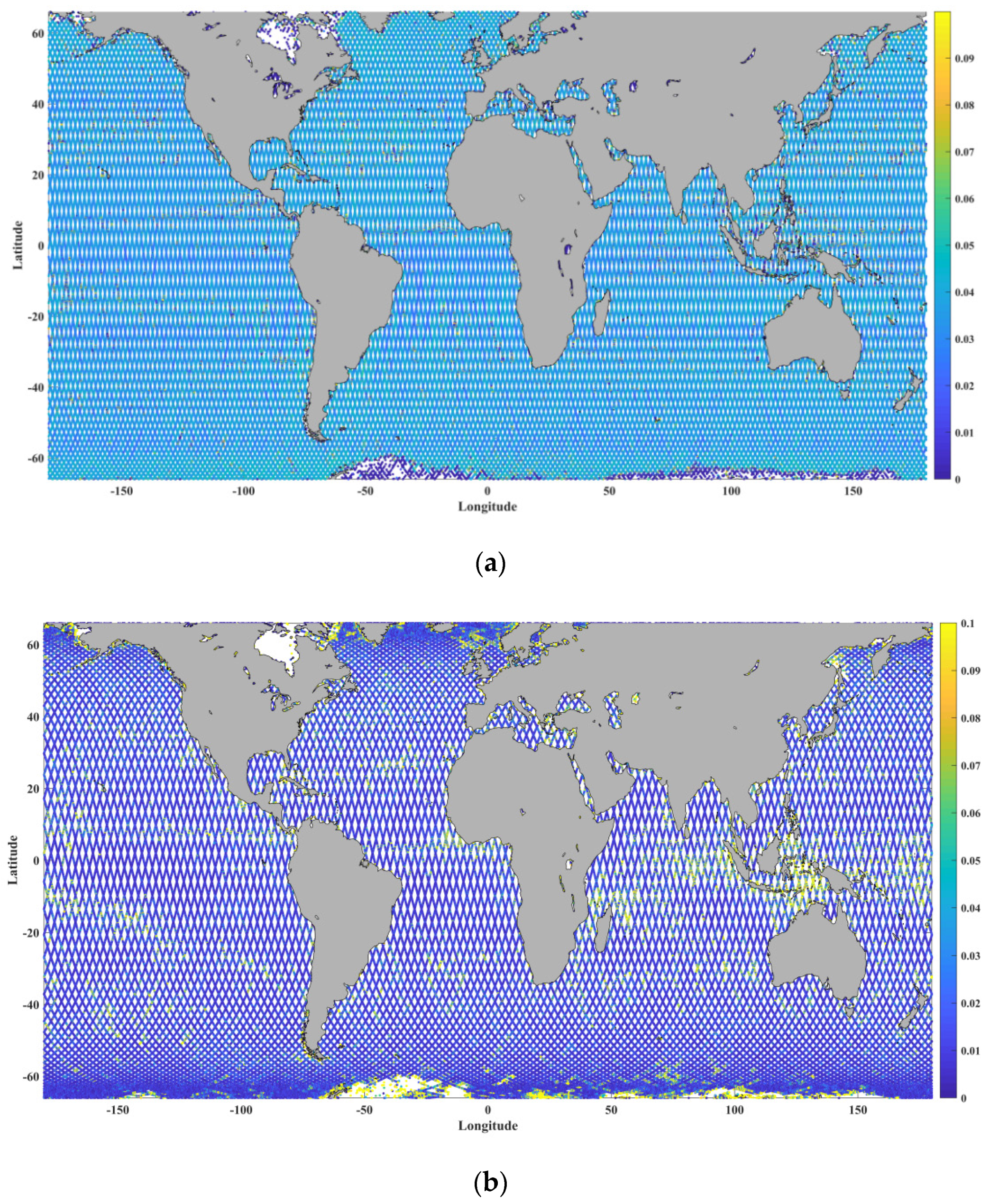Figure 9 shows the comparison of the geographic distribution of the mispointing square between HY-2B and Jason-3. It can be seen from the Figure 9 that the mispointing angle of Jason-3 (Figure 9b) is larger than that of HY-2B (Figure 9a) in mid and low latitude and some nearshore areas. It may be that Jason-3′s orbit control is not as good as HY-2B.

The mispointing angle distributions of the Jason-3 satellite during the period ranging from 31 October 2018 to 5 January 2020 are detailed in Figure 10a, which represent the latest observational data of the Jason-3 satellite which could obtained at the time this study was conducted. The average mispointing angle of one pass was 0.279. Therefore, if this was considered to be valid at less than 0.15 deg² [18], then the mispointing angles of the Jason-3 satellite could be assumed to be mainly distributed between −0.0075 and 0.025 deg² after two mispointing angles greater than 0.15 deg² abnormal pass were deleted. The corresponding standard deviation ranged between 0.017 and 0.118 deg², as shown in Figure 10b.

Generally speaking, the average mispointing angle per pass of the HY-2B satellite was larger than that of the Jason-3 satellite. However, the standard deviation was smaller than that of the Jason-3, as shown in Figure 11.

Therefore, in accordance with the aforementioned analysis results, the short-term variability in the mispointing angles of the HY-2B were found to be closer to zero, which indicated strong stability in the time and geographical distributions. These performance results ensured the reliable estimations of the HY-2B altimeter parameters. In summary, when compared with the Jason-3 satellite, it was confirmed that the HY-2B mispointing angles showed greater stability.

5.2. Backscatter Coefficients and Wind Speeds

At present, in the assessments of the backscatter coefficients of the satellite radar altimeters, the most commonly used method is to compare the backscatter coefficients measured by the new loads with the backscatter coefficients measured by the calibrated satellite radar altimeter day-by-day over a long period of time [10,13,15]. Then, following the comparison process, the accuracy of the backscatter coefficients of the new loads will be significantly reflected.

In the present study, in order to more accurately evaluate the backscatter coefficients of the sub-satellite points measured by the HY-2B satellite’s radar altimeter, a cross assessment method was adopted. In addition, the backscatter coefficients observed by the Jason-3 satellite were selected as the assessment references.

The time delay when the crossover points were selected was one day. The backscatter coefficient distributions observed by the HY-2B and Jason-3 satellites were found to be very similar. However, the mean difference between them was approximately 0.07 dB, and the standard deviation was approximately 0.25 dB, as shown in Figure 12.

Figure 13a,b show this study’s comparison results of mean and standard deviation of the backscatter coefficients at the crossovers of the HY-2B and Jason-3 satellites, respectively. It can be seen in the figures that both the mean and standard deviations of the backscatter coefficients indicated that the backscatter coefficients observed by the two satellites were very close. However, they also differed, which was similar to the results described in Section 4.

At the present time, the inversion model functions of altimeter wind speeds are purely empirical. The most commonly used algorithm models are the Gourrion Algorithm [19] and the Collard Lookup Table [20]. The main idea of the models is to calculate the wind speeds according to the relationship with the backscatter coefficients and significant wave heights of the Ku band.

The wind speed inversion algorithm of the HY-2B satellite radar altimeter uses the following two-parameter model proposed by Gourrion et al. [19]:

$$U_{10}=\frac{Y-a_{U_{10}}}{b_{U_{10}}}$$

(1)

$$Y={\left[1+\exp \left(-\left(\overrightarrow{W_y}\overrightarrow{X}+\overrightarrow{B_y}\right)\right)\right]}^{-1}$$

(2)

$$\overrightarrow{X}={\left[1+\exp \left(-\left(\overrightarrow{W_x}{\overrightarrow{P}}^T+{\overrightarrow{B_x}}^T\right)\right)\right]}^{-1}$$

(3)

where U₁₀ represents the wind speed 10 m away from the sea surface; P indicates the normalized matrix of the SWH and Sig0 with the dimension of 1 × 2; a_U10 and b_U10 are the wind speed coefficients; $\overrightarrow{W_x}$, $\overrightarrow{W_y}$, $\overrightarrow{B_x}$, and $\overrightarrow{B_y}$ represent the undetermined model parameter matrix with the dimensions of 2 × 2, 2 × 1, 1 × 2, and 1 × 1, respectively. The algorithm not only considered the approximate inverse relationship between the sea surface wind speed and the backscatter cross sections, but also introduced the effects of the significant wave heights on the wind speeds. The undetermined parameters in the aforementioned model determined by the neural network model are detailed in

Table 3. Gourrion model parameters.

Parameter	a	b
backscatter coefficient (Sig0)	−0.34336	0.06909
Significant wave height (SWH)	0.08725	0.06374
Wind speed (U10)	0.1	0.02844

and

Table 4. Gourrion model parameters.

Parameter	Matrix Elements
$\overrightarrow{W_x}$	−33.95062	−11.03394
	−3.93428	−0.05834
$\overrightarrow{W_y}$	0.54012	10.40481
$\overrightarrow{B_x}$	18.06378	−0.37228
$\overrightarrow{B_y}$	−2.28387	…
$\overrightarrow{P}$	${\mathrm{a}}_{\mathrm{Sig}0}+{\mathrm{b}}_{\mathrm{Sig}0}{\mathrm{Sig}}_0$	aSWH + bSWHSWH

.

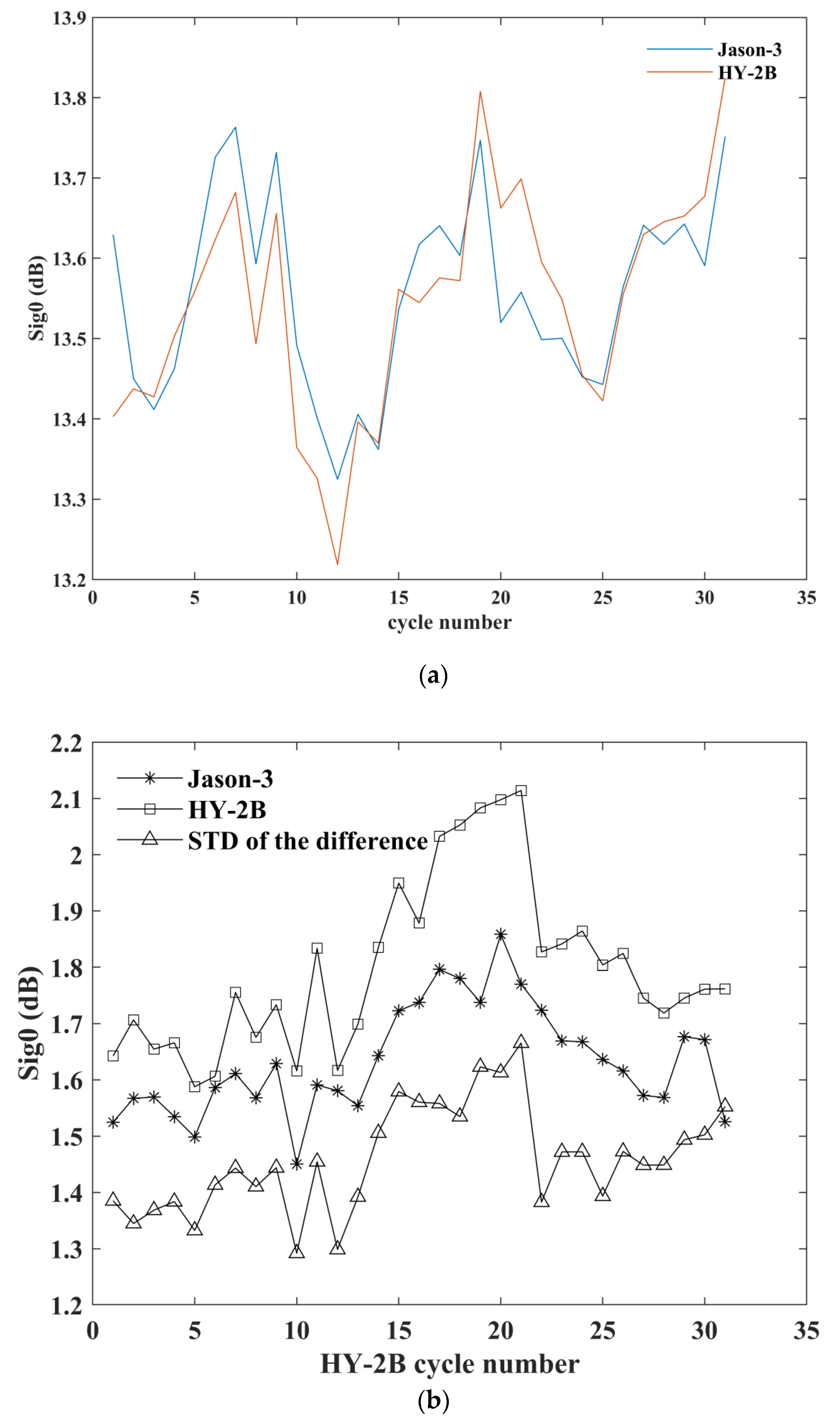
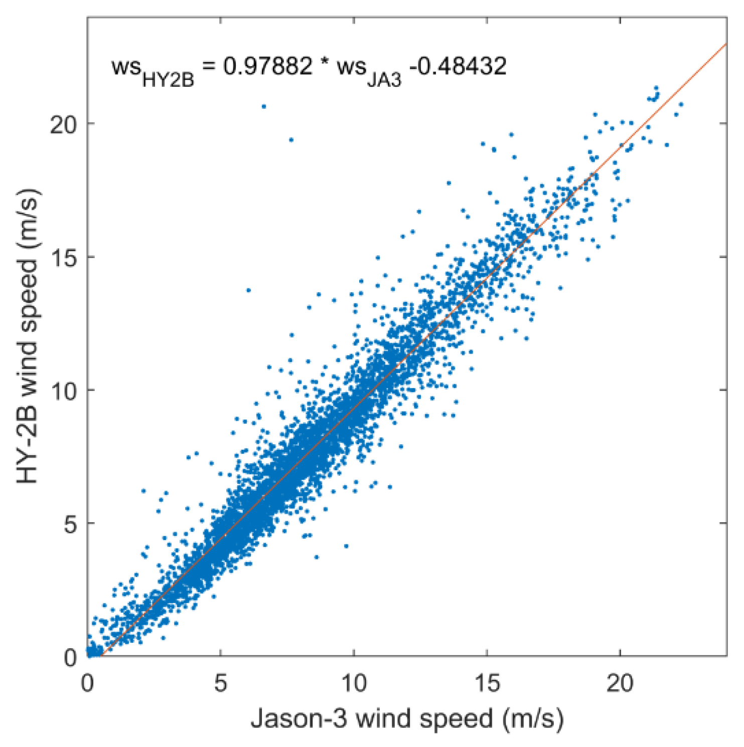
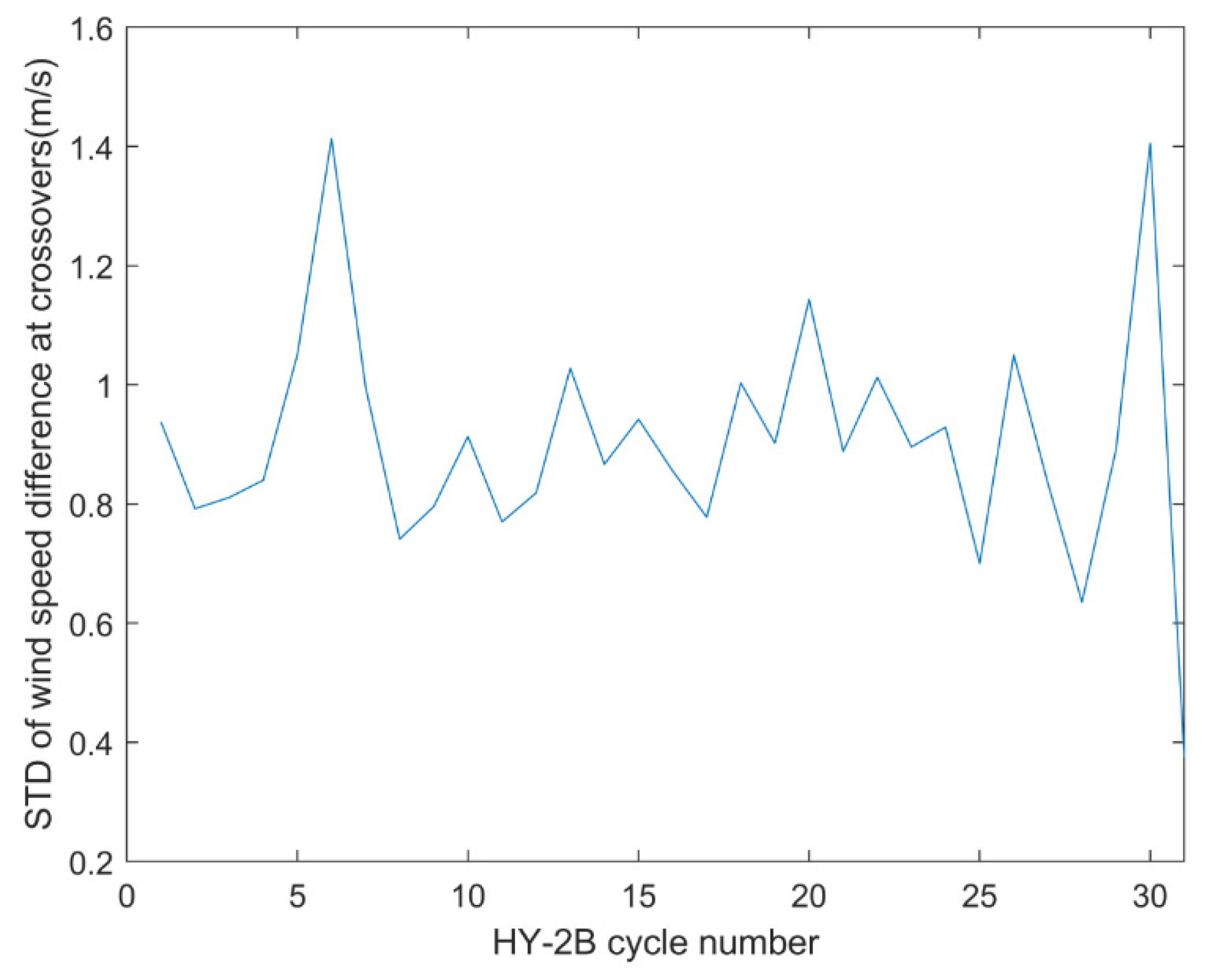
The wind speed comparison results of the HY-2B and Jason-3 satellites revealed that the wind speeds obtained by the HY-2B were slightly smaller than those obtained by Jason-3. However, it was found that there was good consistency between the two satellites, as shown in Figure 14 and Figure 15. The maximum difference of the standard deviation between HY-2B and Jason-3 cycle by cycle is 1.4 m/s.

5.3. Significant Wave Heights (SWH) and Sea State Bias

Satellite radar altimeters are active microwave remote sensors pointing at nadir. This type of equipment is able to vertically transmit electromagnetic pulses to sea surfaces and then receive backscattered echoes from the sea surfaces for observational purposes. The echo waveforms of satellite radar altimeters contain information regarding significant wave heights [21,22,23,24,25]. The significant wave heights can be estimated from the slopes of the leading edges of the return pulses [25,26,27].

In the present study, a maximum likelihood estimator (MLE4) [28] with four free parameters (range, significant wave height, power, and antenna mispointing angle) was used to estimate significant wave heights from the average return signals contained in the waveforms of the HY-2B satellite.

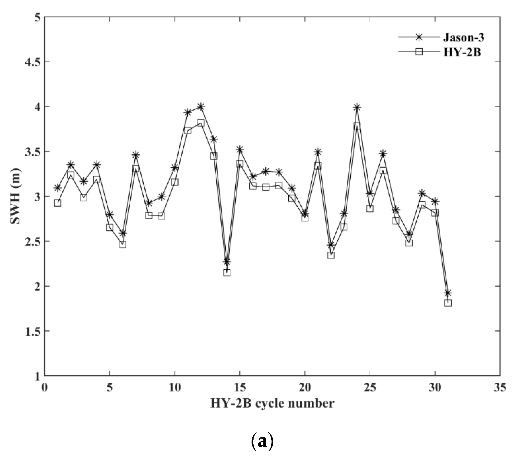
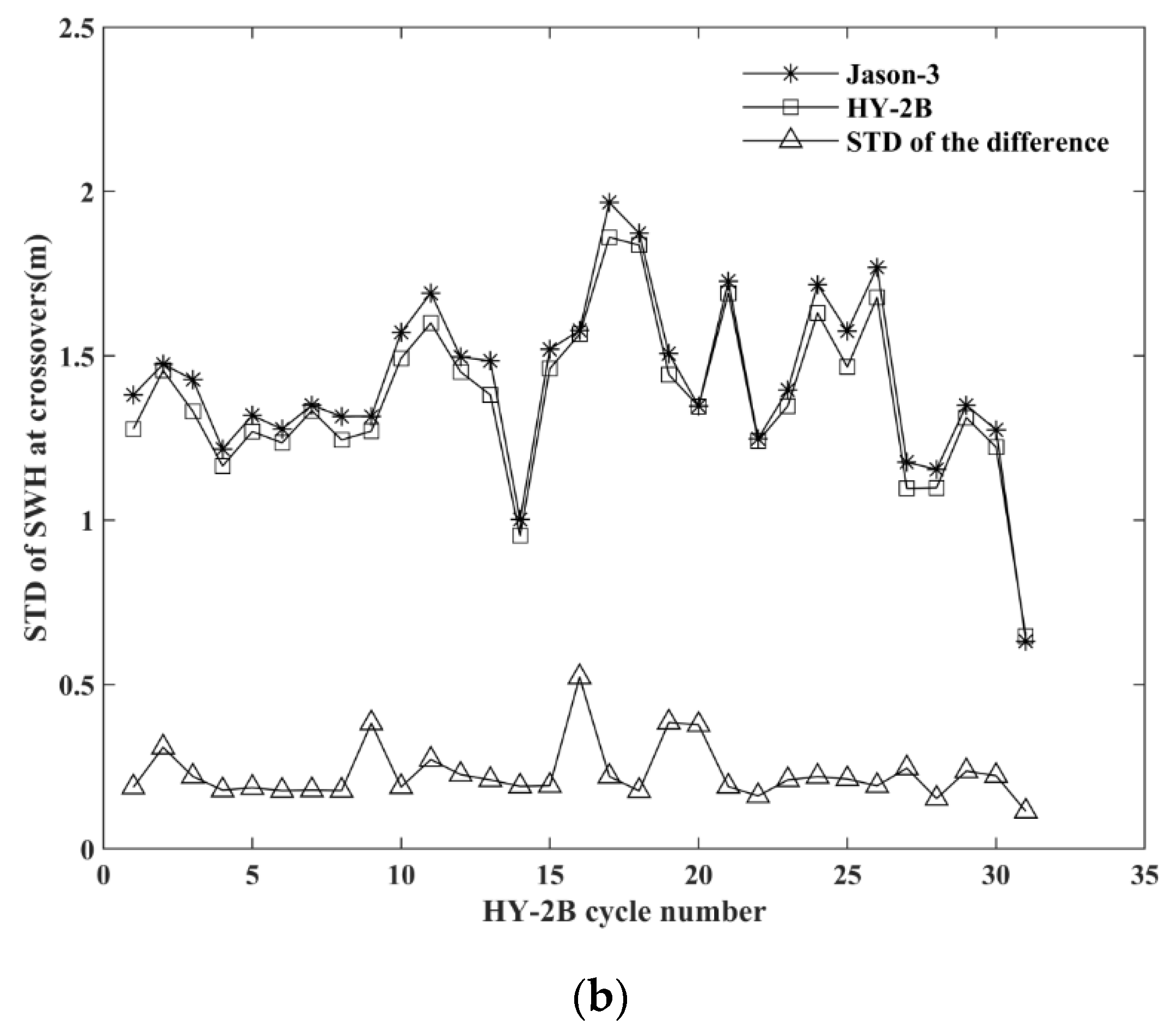
As shown in Figure 16, the standard deviations of the difference were 12 cm to 52 cm from cycle 1 to cycle 31. With respect to the Jason-3 satellite, as shown in Figure 17, the significant wave height bias shows uniform distribution remaining almost completely constant at approximately 0.15 m, as shown in Figure 16.

Electromagnetic (EM) bias, skew bias, and tracking bias are collectively referred to as sea state bias (SSB) [29], with typical values ranging between −1% and −4% SWH [30]. The mechanism of the sea state bias is complex. The RMS can reach 2.0 cm when the wave heights are 2 m in the TOPEX/Poseidon altimeter [31]. Meanwhile, the total RMS in the T/P altimeter is only 4.1 cm. Therefore, it can be seen that its proportion in the total RMS is very large. In the Jason-1 satellite altimeter, the sea state bias had replaced the orbit errors to become the most important error source [30]. The SSB model which was derived in theory was found to not be suitable for the corrections of sea state bias of the satellite altimeters. Therefore, for the HY-2B satellite, a non-parametric correction method was adopted for the sea state bias. This empirical fits model was used in Jason-3 data processing also.

The sea state bias of the HY-2B and Jason-3 satellites had a fixed difference of approximately 1 cm. It was observed that the sea state bias of the Jason-3 was greater than that of the HY-2B. This was determined to be related to the fact that the significant wave heights and sea surface wind speeds of the Jason-3 satellite were generally greater than those of the HY-2B satellite. At the crossover points, the maximum standard deviation is 1.8 cm, as shown in Figure 18, which is the larger term in the height measurement error corrections. However, overall, the HY-2B sea state bias was approximately −3.5% that of the significant wave heights which was basically consistent with the sea state bias of many other satellite radar altimeters.

6. Sea-Level Performances

The purpose of this research study was to evaluate the performance of the entire HY-2B altimeter system. This required the evaluation of the quality of each parameter of the Level 2 product, particularly if it was possible to use those parameters in the SSH calculations. However, it was found that if the tides, dry tropospheric path delay error corrections, and wet tropospheric path delay error corrections were evaluated, the task became too cumbersome and lengthy. Therefore, this study chose to directly evaluate the sea surface heights (SSH) and sea-level anomalies (SLA), since all of the altimetric error corrections could be used in the calculations of the SSH and SLA. It was found that if one of the aforementioned displayed a large height measurement error, it directly reflected the poor accuracy of the SSH and SLA results.

The quality of the altimeter data and the performance levels of the sea level measurements were successfully evaluated by analyzing the sea level differences at the satellites’ crossover points. Ideally, the mean values of the sea level differences at the crossover points would have been close to 0, and the standard deviation would be very small. Crossover assessment methods had been previously used in the accuracy assessments of the satellite radar altimeter products including the TOPEX/Poseidon, Jason-1/2/3, Sentinel-3A, SARAL, HY-2A, and so on [7,8,9,10,11,12,13,14,15].

Prior to the cross assessments, it was necessary to clarify the models and algorithms used in height measurement error corrections of the HY-2B and Jason-3 satellites.

Table 5. Main correction methods for altimetry errors of the HY-2B and Jason-3 satellites.

Correction	Jason-3	HY-2B
Dry troposphere	Model, ECMWF(European Centre for Medium-Range Weather Forecasts)	Model, NCEP(National Center for Environmental Prediction)
Wet troposphere	Calibration radiometer	Calibration radiometer
Ionosphere	Dual frequency	Dual frequency
Sea state bias	Non-parameter model	Non-parameter model
Ocean tide	GOT4v8	GOT4.10c
Solid Earth tide	elastic response to tidal potential	elastic response to tidal potential
Pole tide	(Wahr, 1985) [32]	(Wahr, 1985) [32]
Load tide	GOT4v8	GOT4.10c
Atmospheric adverse pressure	Model, ECMWF	Model, NCEP
Version	GDR-D	GDR-A

shows the main height measurement error correction methods of the HY-2B and Jason-3 satellites.

In addition, it was necessary to screen the data, and then select the data which was less affected by land and observation anomalies as the assessment objects. The specific screening criteria were as detailed below [https://www.aviso.altimetry.fr/fileadmin/documents/data/tools/hdbk_j3.pdf].

Parameter validity conditions:

• range_numval_ku 10 ≤ x
• range_rms_ku 0 ≤ x (mm) ≤ 200
• altitude – range_ku −130,000 ≤ x (mm) ≤ 100,000
• model_dry_tropo_corr −2500 ≤ x (mm) ≤ −1900
• rad_wet_tropo_corr −500 ≤ x (mm) ≤ −1
• iono_corr_alt_ku −400 ≤ x (mm) ≤ 40
• sea_state_bias_ku −500 ≤ x (mm) ≤ 0
• ocean_tide_sol1 −5000 ≤ x (mm) ≤ 5000
• solid_earth_tide −1000 ≤ x (mm) ≤ 1000
• pole_tide −150 ≤ x (mm) ≤ 150
• swh_ku 0 ≤ x (mm) ≤ 11,000
• sig0_ku 7 ≤ x (dB) ≤ 30
• wind_speed_alt −0 ≤ x (m/s) ≤ 30
• off_nadir_angle_wf_ku −0.2 ≤ x (deg2) ≤ 0.64
• sig0_rms_ku x (dB) ≤ 1
• sig0_numval_ku 10 < x

In addition, in order to reduce the impacts of changes in the oceanic conditions on the assessment results, a time delay of 3 days was chosen when evaluating the sea levels. The maximum time intervals for the assessments of the crossovers of the sea level measurements tend to be slightly different among different researchers, and may include 10 days, 3 days, 30 min, and so on, depending on the study criteria [7,8,9,12,13,14].

There were two basic concepts to be introduced in this study: sea surface heights (SSH) and sea-level anomalies (SLA).

The sea surface heights (SSH) indicate the distances of sea surfaces above the reference ellipsoid. In other words, they represent the differences in the altimeter ranges from the satellite altitudes above the reference ellipsoid and those calculated by subtracting the corrected ranges from the altitude measurements.

For example, SSH calculations in this study were defined as follows:

SSH = Altitude (Orbit) − (Altimeter Range + ∑Corrections)

Where the “Altimeter Range” is the range which is corrected for instrumental effects; and

∑Corrections = dry tropospheric path delay correction + Radiometer wet tropospheric path delay correction + Sea State Bias correction + inverse barometer correction + dual frequency ionospheric correction + ocean tide correction (including loading tide) + earth tide correction + pole tide correction.

Therefore, the sea level anomalies are the bias of the sea surfaces relative to the mean sea levels, and comprise the main data sources of oceanic dynamic research and dynamic phenomenon observational processes. The mean sea level of the HY-2B was mss_cnes_cls2015 (https://www.aviso.altimetry.fr/).

6.1. HY-2B Satellite Mono-Mission Crossovers

Multiple satellite radar altimeters have been comprehensively evaluated by means of mono-mission crossovers in order to achieve high measurement accuracy [7,33,34]. This study’s comparison of the HY-2B satellite’s sea-surface heights and sea-level anomalies at the crossover points of the lifting orbits clearly indicated the stability of the HY-2B satellite’s radar altimeter observations, as well as the existence of time scale bias, measurement accuracy, and other valuable information.

Figure 19a shows the cycle by cycle mean distributions of the differences in the HY-2B sea surface heights at the crossover points of the ascending and descending orbits. It can be seen in the figure that during all 35 cycles, the differences in the average sea surface heights at the crossovers of the ground tracks were less than 4 mm. These results confirmed the observation stability of the HY-2B satellite’s radar altimeter performance. It was also proven that the accuracy of the GDR products of the HY-2B satellite’s radar altimeter had displayed little differences in time and space. There were no time scale bias problems as observed in the HY-2A satellite [3,4,5].

Figure 19b shows the mean distributions of the sea level anomalies differences at the crossovers of ascending and descending ground tracks. The results indicated that the standard deviation of the sea-level anomalies of the HY-2B and Jason-3 satellites were less than 5.7 cm. These results were found to be similar to or superior to those obtained by the Jason-1, Jason-2, and Sentinel-3A satellites.

6.2. Cross-Calibrations with the Jason-3 Satellite

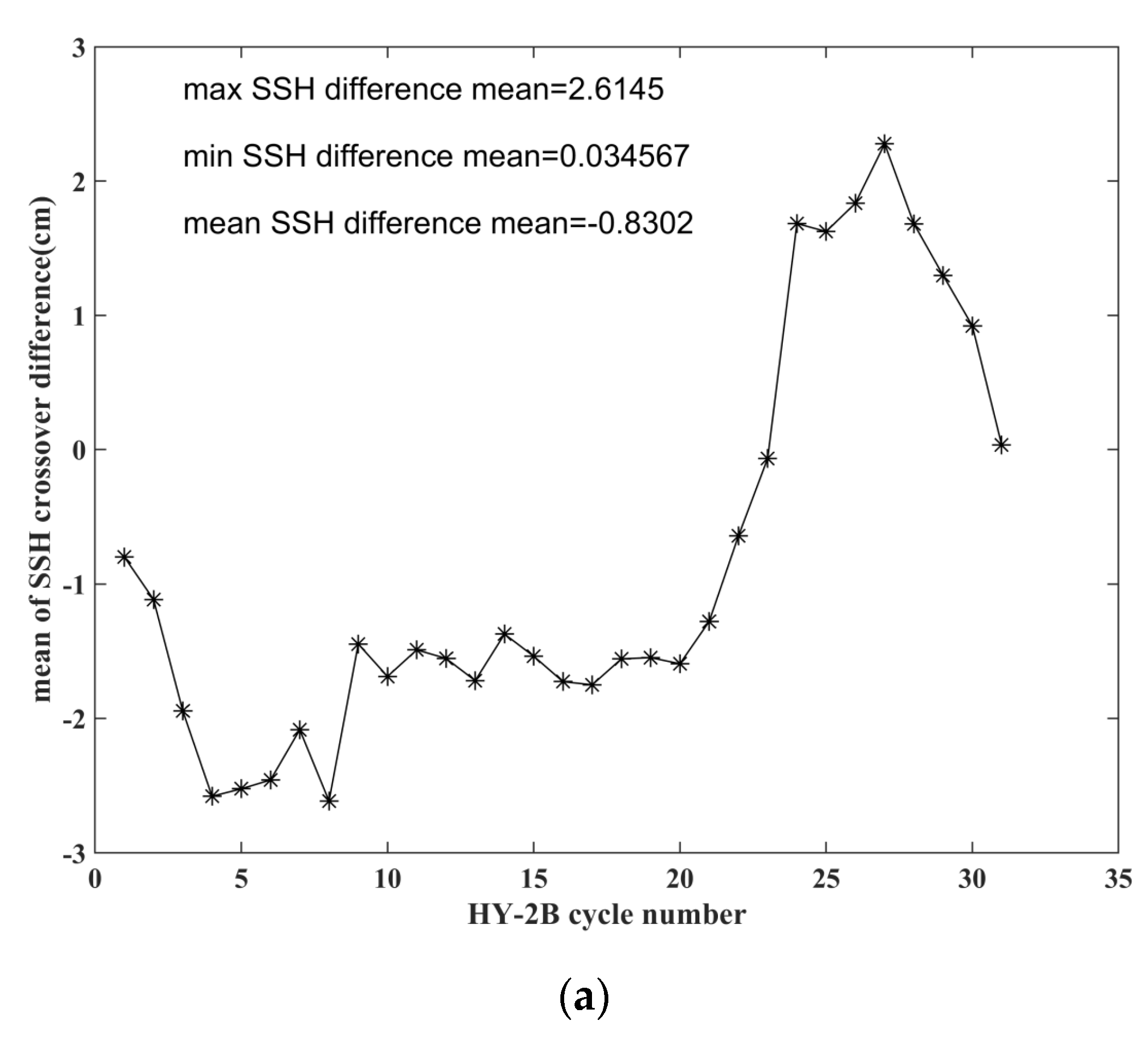
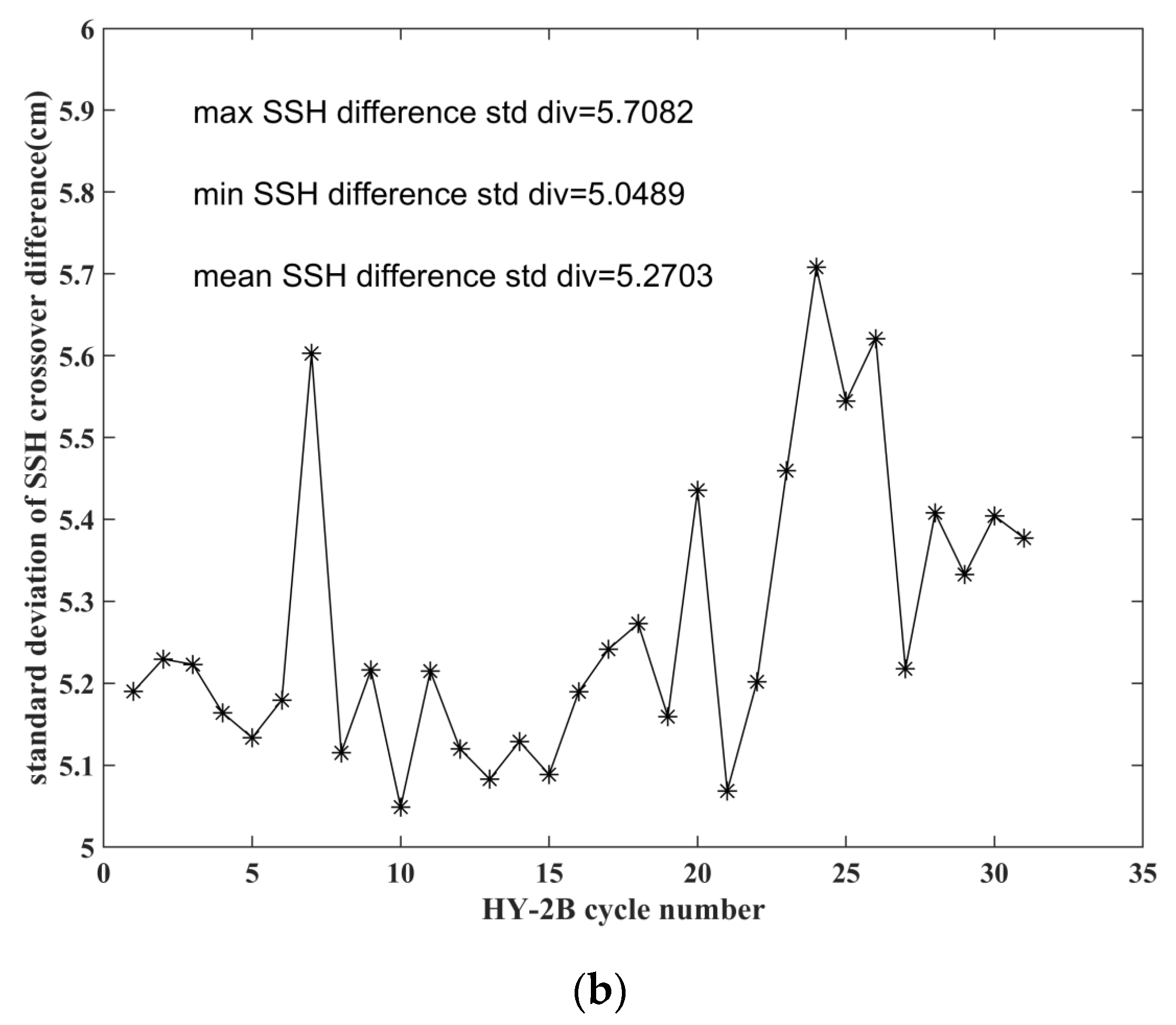
In order to more clearly evaluate the accuracy of the sea-level measurements achieved by the HY-2B satellite’s radar altimeter, the sea-level and sea-level anomaly measurement results of both the HY-2B satellite and the Jason-3 satellite were compared for the period ranging between 30 October 2018 and 5 January 2020. The comparison was made according to the observational cycle of the HY-2B satellite. The differences in the standard deviation of sea surface heights and sea level anomalies during each observational cycle were compared.

It was found that during the 31 observational cycles, the maximum difference of the mean value of the sea surface height differences at the crossover points was 2.61 cm, as shown in Figure 20a. The differences in the standard deviation of the sea surface heights were found to be minimal, ranging from 5 cm to 5.7 cm, as shown in Figure 20b.

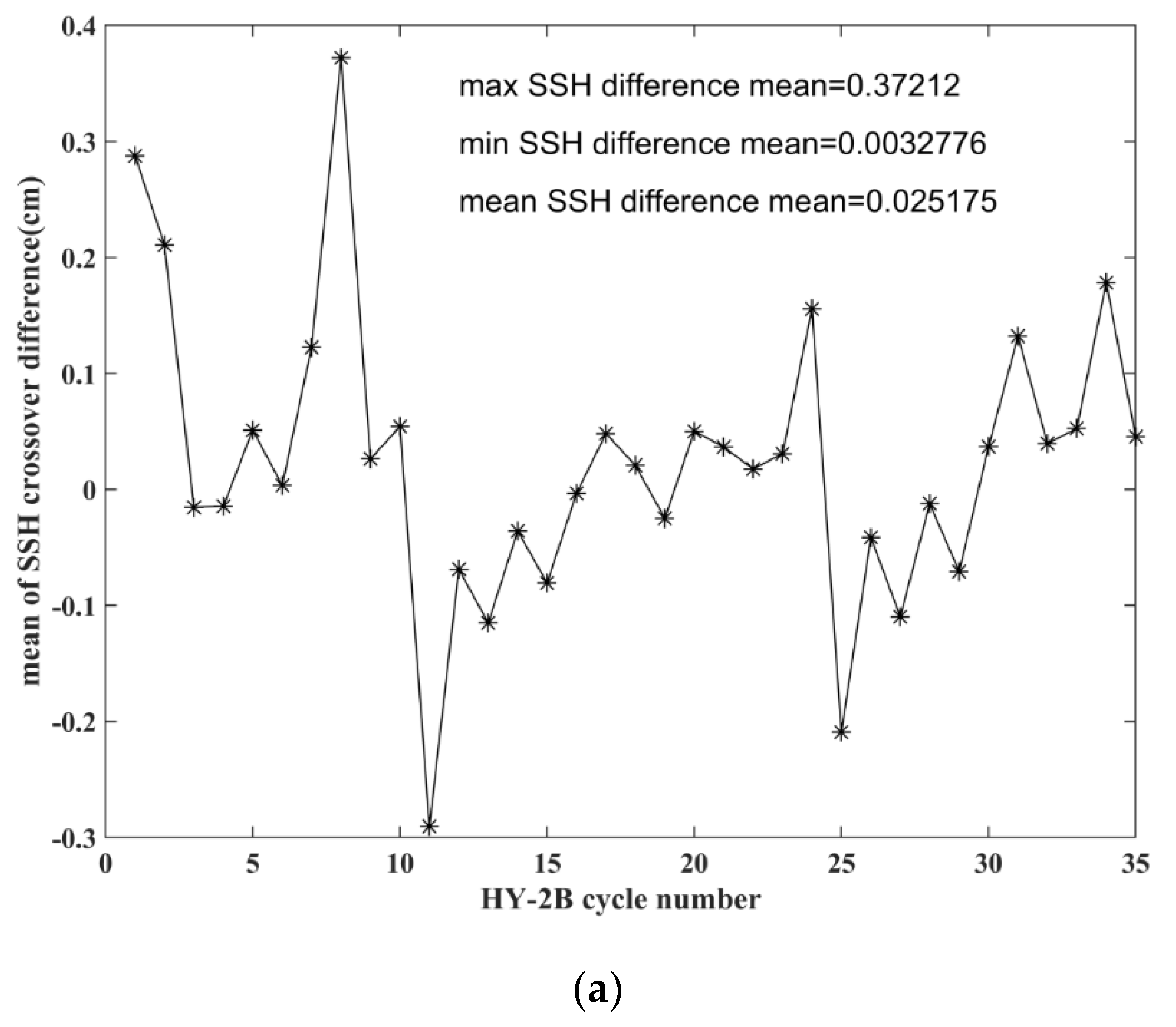
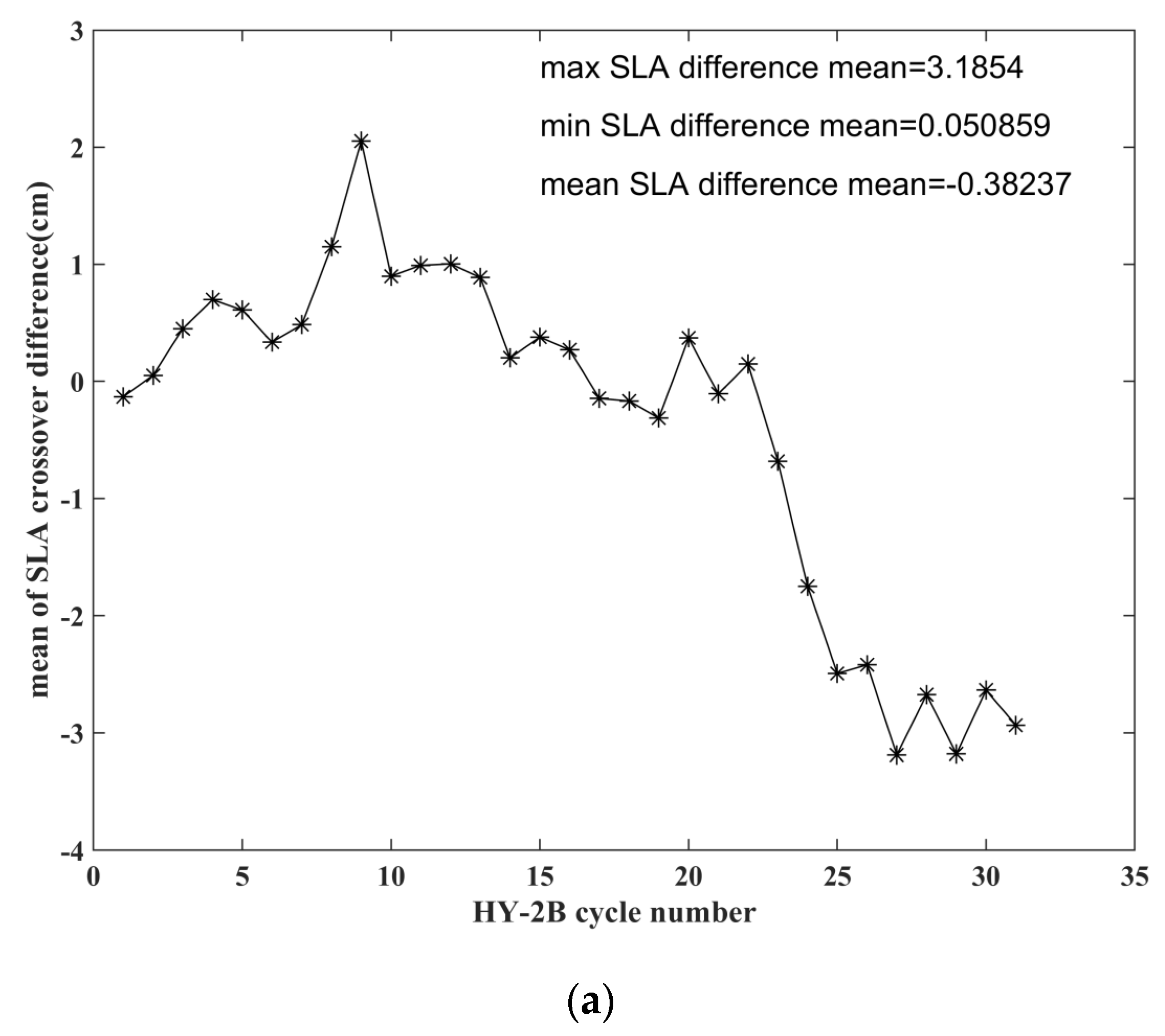
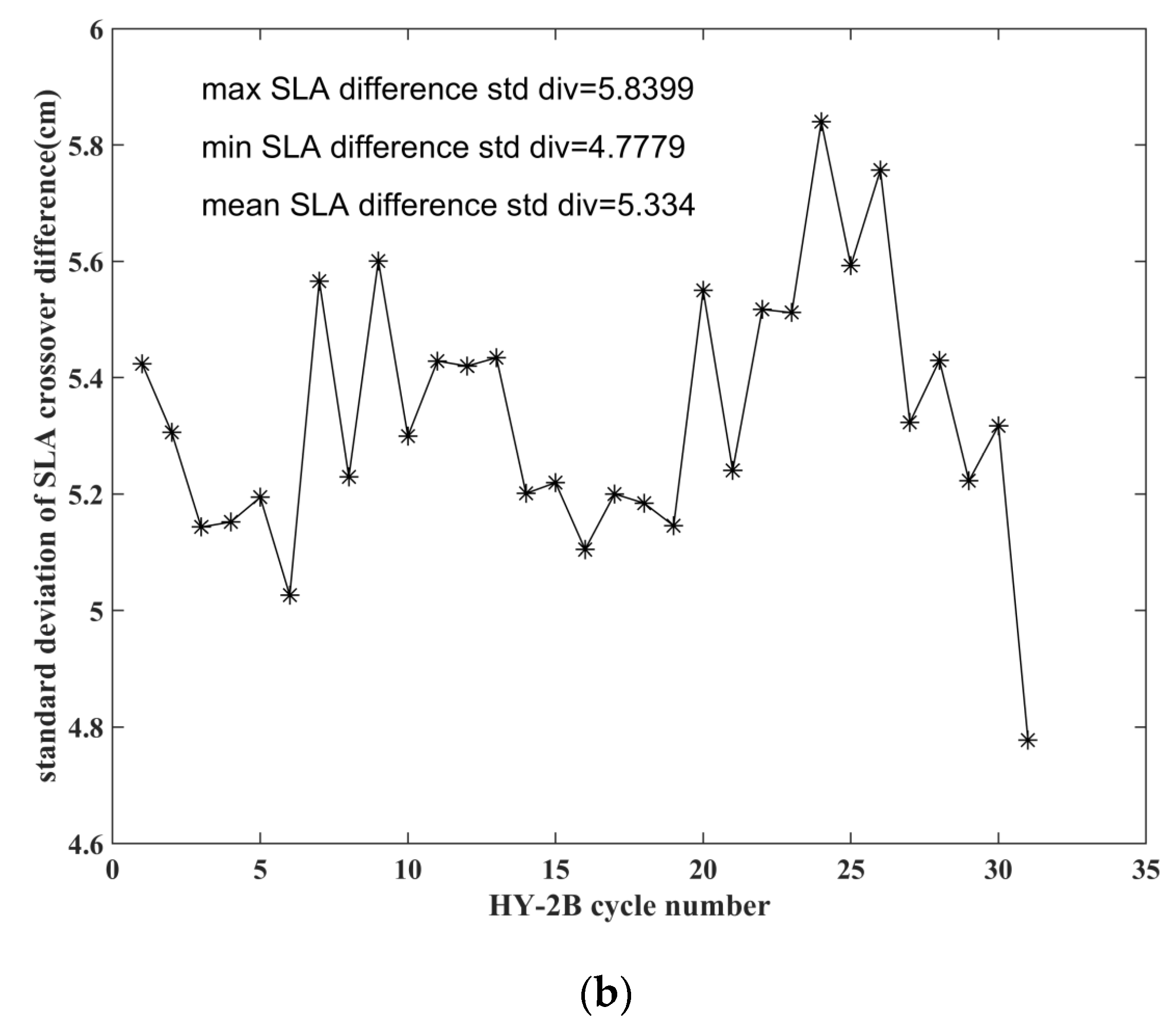
The mean values of the cycle-by-cycle sea level anomaly differences based on the HY-2B satellite cycles were found to have a maximum difference of 3.2 cm, as shown in Figure 21a. In addition, the standard deviation of the sea surface heights displayed only very small differences, as shown in Figure 21b. The maximum difference of the SLA standard deviation was determined to be 5.8 cm, which appeared during the 24th cycle. The minimum value was 4.8 cm, which appeared during the 31st cycle.

The standard deviation of the sea surface heights and sea level anomalies at the crossover points of the HY-2B and Jason-3 satellites were found to be consistent with those of the sea surface heights and sea level anomalies at the mono-mission crossovers recorded by the altimeter of the HY-2B satellite. Those findings confirmed once again that the observations of HY-2B satellite’s radar altimeter were stable, and the accuracy of the product was consistent with that of the Jason-3 satellite.

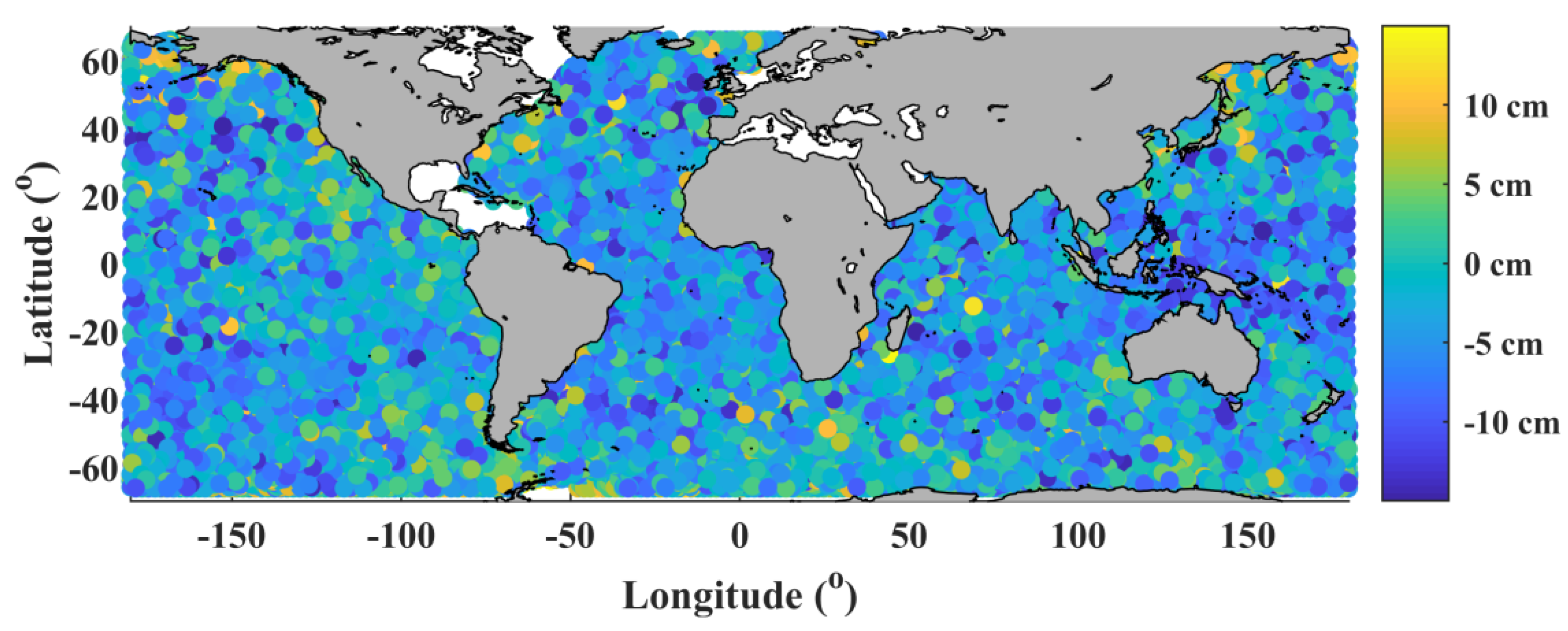
The spatial distributions of the SLA differences at the crossover points of the HY-2B and Jason-3 satellites were very uniform. As shown in Figure 22, there were no significant differences observed between the northern and southern hemispheres resulting from time scale bias. However, in the high-latitude sea areas or near shore shallow water areas, the largest differences observed in the SLA were more than 10 cm.

6.3. Sea-Level Anomalies (SLA) Power Spectra

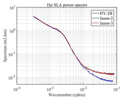
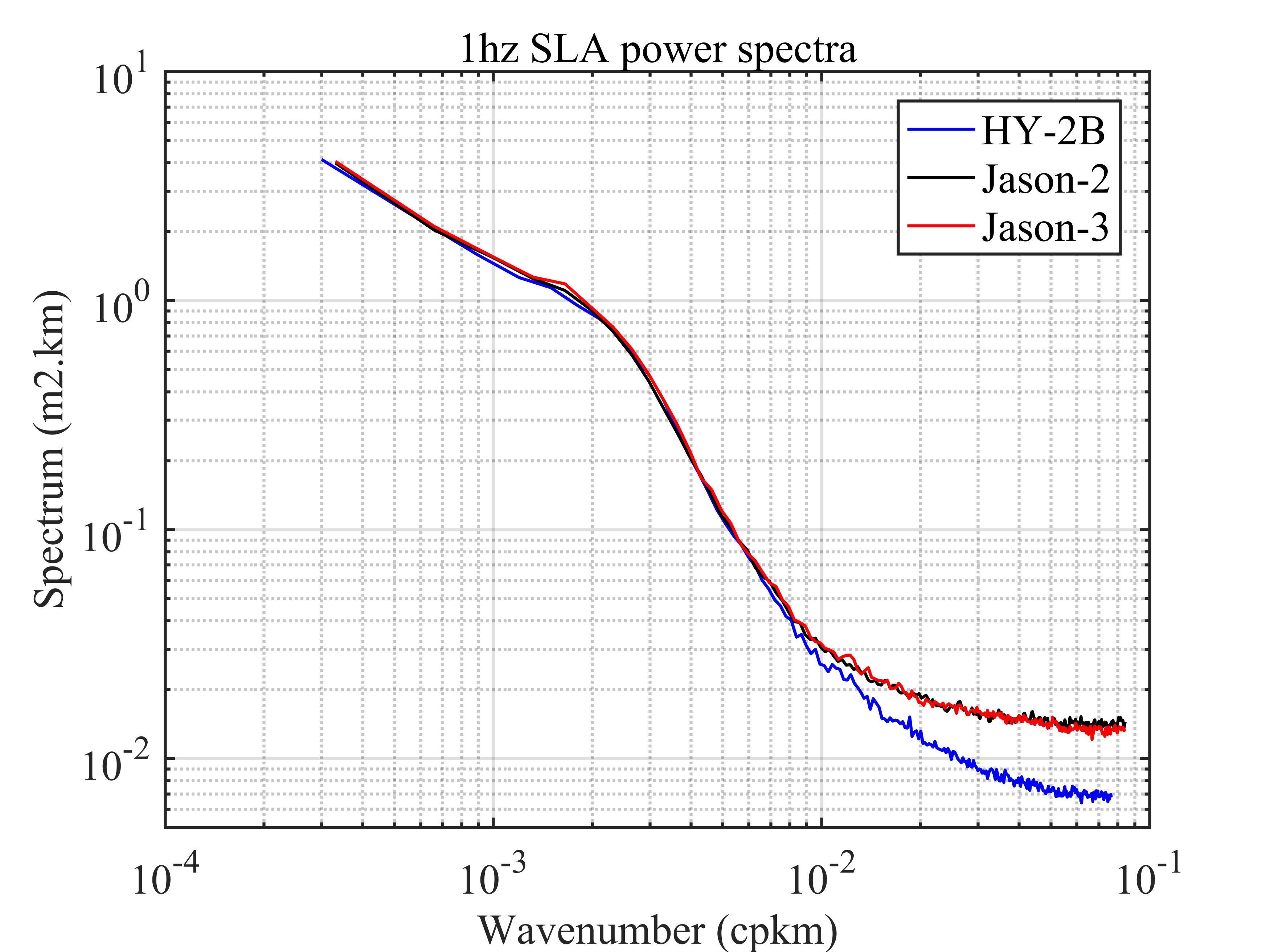
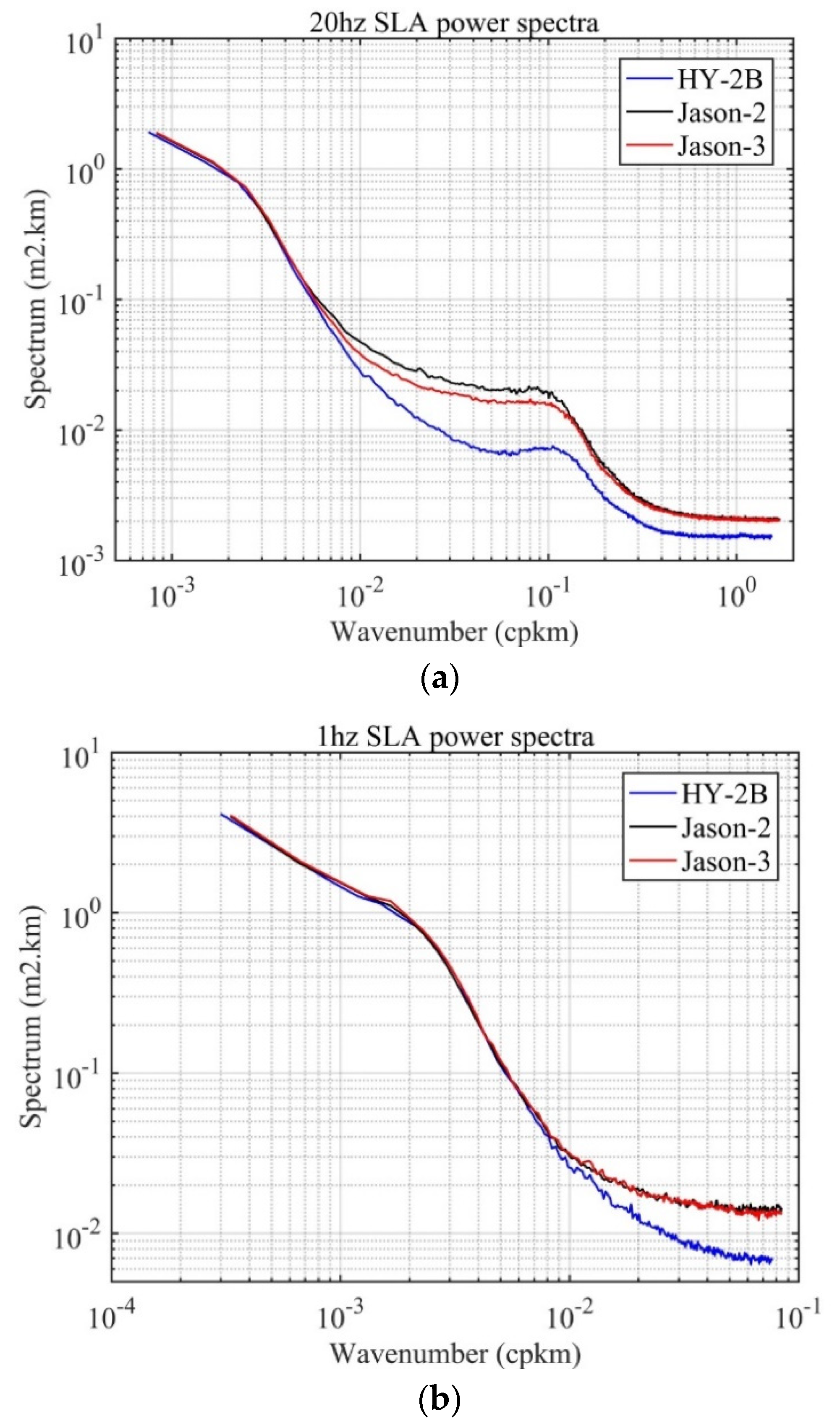
To assess and compare the performance of missions, spectral analysis of SLA is widely used in the altimetry community. In order to further illustrate the mean noise measurements over the global oceans, this study detailed the along-track SLA power spectrum densities (PSD) for the 20 Hz data, explicitly separating the HY-2B, Jason-2, and Jason-3 satellites, as well as for the 1 Hz HY-2B, Jason-2, and Jason-3 satellite data. In addition, the wave numbers were computed in terms of cycles per km.

SLA power spectra computed using Jason-2/3 and HY-2B data over the ocean from 30 October 2018 to 27 February 2019. Periodogram power spectral density estimating method was used to compute DFT (discrete Fourier transform) on a logarithmic frequency scale. No zero-padding, rectangular window was used in this process. It was found in this study that there was an interesting feature of a spectral hump, which appeared in the 20 Hz data within the wavelength range between 3 km and 50 km, as shown in Figure 23a. It has been proved that the hump originates in a response to inhomogeneities in backscatter strength through an analysis of simulations and actual data from multiple missions [34]. This spectral hump has been well documented in previous altimetry literature, and reflects one of the main limiting factors of satellite altimetry in regard to resolving small-scale features. As expected, the spectral hump was not visible in the 1 Hz data, as shown in Figure 23b.

It was noted in this research investigation that the noise floor for the 1 Hz data from the HY-2B satellite was smaller than that of the Jason-2 and Jason-3 satellites, which were approximately 2.3 cm and 2.9 cm, respectively. Both spectra showed similar spectral characteristics for the right part of the PSD. In regard to the right part of the PSD, this study found that the noise level of the HY-2B was lower than that of the Jason-2 and Jason-3 satellites, as shown in Figure 23b.

7. Conclusions

According to the comparison and analysis results obtained in this study, and based on the long-term monitoring and comparisons of the Level 2 GDR products of the Jason-3 satellite radar altimeter, it was concluded that the HY-2B altimeter data products displayed good stability and high accuracy. The differences in the SSH between the HY-2B and Jason-3 satellites were less than 3 cm at their ground-track crossovers. All of the achieved good results indicated that the data quality of the HY-2B satellite radar altimeter was high, and was basically the same as that of the international equivalent satellite radar altimeter of the Jason-3 satellite. Finally, the HY-2B high-precision altimeter satellite was confirmed to have met oceanic circulation and climate research requirements similar to the Jason satellite series’ radar altimeter systems.

Although the accuracy of the Level 2 products of the HY-2B satellite’s radar altimeter was determined to be very high according to this study’s assessments, the inversion results of the backscatter coefficients, sea surface wind speeds, significant wave heights, and so on were found to have a fixed bias from the Jason-3 satellite. It was assumed that the fixed bias was not significantly related to the inversion method, but rather related to the compensation of the instrument. Therefore, in the next version of the product, this study recommends that the fixed corrections be resolved.

The altimetry accuracy of HY-2B is better than that of Jason-3 when the noise of HY-2B is lower. In addition there is almost no difference for the correction of height measurement error between HY-2B and Jason-3. According to the calculation formula of SSH and SLA, the precision of SSH and SLA should be better than Jason-3. But based on the analysis of this paper, the products of SSH and SLA accuracy of the two missions is almost the same. There should be two reasons for this result: first, HY-2B satellite is not equipped with Doris orbit determination system, only dual-frequency GPS data are used for precise orbit determination, and the precise orbit determination accuracy cannot reach the accuracy of Jason-3; second, the current product accuracy of the correction radiometer on the HY-2B satellite is close to the accuracy of the wet troposphere path delay correction calculated by using the model and NCEP (National Center for Environmental Prediction)data (there is no comparison in this paper). Clearly, it does not give full play to the efficiency of radiometer calibration. In order to improve the accuracy of SSH measurements, we have to improve the accuracy of calculating the wet tropospheric path delay by using the brightness temperature measured by calibrated radiometer. At the same time, the precision of precise orbit determination should be improved.

At the same time, the comparisons and validations of the acquired data will need to be continued in order to monitor all of the relevant parameters, SSH, and SLA, over time. In particular, it will be necessary to cooperate with the field buoys and other measurement results for the purpose of conducting comparisons. Then, following the necessary inspections, the HY-2B satellite radar altimeter products can be utilized as data sources for the inspections of other altimeter satellite products. Finally, the data can also be utilized for the inspections and calibrations of the products obtained by the HY-2C satellite’s radar altimeter set to be launched in the near future, as well as the subsequent HY-2D satellite’s radar altimeter products.