Abstract
In this paper, we applied the re-analysis data cobe-SST (cobe-sea surface temperature) and Global Land Data Assimilation System (GLDAS) surface soil moisture (SM) data from 1961 to 2011 by using regional correlation analysis and time series causality analysis to trace annual variations in and identify the abnormal relationship of sea surface temperature (SST) in the eastern China Sea and SM in eastern China (EC). We also used satellite Moderate Resolution Imaging Spectroradiometer (MODIS) SST and AMSR-E SM data to examine the correlation of SST and SM in EC from 2004–2009. The results show that the SST in the eastern China Sea has experienced a warming trend since 1987, whereas the SM in EC has shown a drying trend since 1978. Before 1967 and after 1997, SST and SM changed during opposite phases, whereas from 1967 to 1997 they changed during the same phase. The differences between them may result from the abnormal summer precipitation causing abnormal SM. According to the regional correlation analysis, SST of the East China Sea is significantly related to SM in the southeast coastal area, and temporal sequence causality analysis shows that SST is correlated with and has higher influence on SM than vice versa. SM during spring and autumn shows a similar correlation with SST during the four seasons, so that SM in spring and autumn is positively correlated with SST in autumn and negatively correlated with SST in other seasons. SM in summer and winter correlated with SST in the four seasons, contradicting the foregoing conclusions. All these findings indicate that the thermodynamic state of the eastern China Sea has affected SM in EC.
1. Introduction
All creatures on the earth live on its surface, with air, water, sunlight, soil, and rocks in the biosphere providing all the necessary conditions for life activities. The water cycle is closely related to weather and climate change. The ocean has a very great heat capacity and influences atmospheric circulation and water vapor through the evaporation of its surface layer, but because air–sea interaction is a relatively slow process, the ocean’s influence on climate is gradual. Land surface accounts for only 30% of the earth’s whole surface, and its heat capacity and thermal inertia are quite small, so that land–gas interactions are a relatively rapid process influencing land surface moisture, vegetation, and snow. Land surface conditions are closely related to local weather and changes to the climate system, as a result of which the transfer of momentum can affect climate change regionally and even globally.
Abnormal changes in meteorological factors, such as precipitation and soil moisture (SM), in eastern China (EC) are closely related to the east Asian monsoon [1]. Some research [2] has shown that the frequency of drought and flood disasters in China is related to interannual changes in the east Asian monsoon climate system that influences the ocean-land-atmosphere subsystems, as well as interannual and interdecadal changes of sea surface temperature (SST) in the central and eastern Pacific. Thus SST is an important reference factor for the study of climate change, and the eastern China sea, which is located in the western Pacific Ocean, directly affects climate change in EC. Recently scholars have learned that China’s offshore waters (the Bohai Sea, Yellow Sea, East China Sea, and South China Sea), as well as other minor seas in the northwest Pacific, have been warming significantly since the 1970s, especially in the area of the East China Sea shelf (Bohai Sea, Yellow Sea, and East China Sea), with adjacent sea areas undergoing especially significant warming [3,4]. Thermal variations in the East China Sea and adjacent seas will inevitably lead to abnormal atmospheric circulation in east Asia, causing climate anomalies in EC, especially changes in precipitation [5], which in turn will inevitably lead to abnormal SM. Many studies have been conducted of the relationship between the thermal variability of tropical oceans or global seas and summer drought and flood in China [6,7,8,9]. However, few studies have examined the abnormal effects of thermal variation on precipitation and surface soil moisture (SM) in China’s coastal areas and adjacent seas, especially the East China Sea.
The high temporal and spatial variability of SM makes it difficult to observe, diminishing temporal and spatial continuity of observation data [10]. Although remote sensing [11,12] has solved the problem of space scale, both microwave and optical angles can detect only the shallow soil, restricting study of deep SM by remote sensing observation. The land surface model is an indispensable tool for the study of SM. Since the 1960s, this model has undergone rapid and successful development. In 1969, Manabe created the simplest bucket schema [13], which gradually developed and increased in complexity, from BATS mode, Sib mode, and Common Land Model (CLM) mode to GLDAS mode—all of which models have their own advantages [14,15,16,17]. Since the development of this model, meteorologists have used it to verify and evaluate its applicability. Simultaneously, a set of SM data has emerged since then. Based on the National Oceanic and Atmospheric Administration (NOAA) SST data of 1958/2001, the European Center for Medium-Term Weather Forecast (ECMWF) ERA40 SM reanalysis data of European weather center, and the precipitation data of 444 stations east of 100° E in China, Gao suggests a significant negative correlation between SM in eastern southwest China and precipitation in the middle and lower reaches of the Yangtze River in summer but a positive correlation with the precipitation in the southeast coastal areas of China [18]. Chen et al. compared the adaptability of SM data of ERA-Interim reanalysis data (ERA) and National Aeronautics and Space Administration (NASA) reanalysis data (MERRA) in the Jiangsu region and found that the two sets of data are more accurate for the simulation of subsurface SM but that there is a certain gap between their description of deep SM and actual observations [19]. Based on SM observation data, Zhu compared and evaluated the applicability of four sets of reanalysis SM data—CFSR, ERA-Interim, NCEP R-1, and NCEP R-2—in China from 2001 to 2010. The results showed that the four sets of reanalysis data describe well the distribution characteristics of regional SM in China and have their own advantages on the time scale [20]. Ma evaluated the reliability of two sets of reanalysis SM data in typical areas: satellite remote sensing inversion of the European Space Agency (ESA) and ERA-Interim of ECMWF. The results showed that the two kinds of SM could describe well the total soil dry and wet changes in the observed area but that there were temporal and spatial differences in the consistency between the mean value and the trend [21]. At the same time, some researchers have focused on GLDAS data, noting their credibility compared with observation data. Cui et al calculated the fusion product of the Global Land Surface assimilation system (GLDAS-NOAH) and the Land Surface assimilation system of the China Meteorological Administration (CLDAS-V2.0) the correlation with and deviation from the observed data, the average correlation R and root mean squared error (RMSE) of surface SM were 0.53 and 0.11, and the average R and RMSE of deep SM were 0.31 and 0.12, indicating that the two models can describe well the shallow SM but that their applicability to deep SM is poor [22]. Ghazanfari et al. defined a new drought index using GLDAS-LSM data, which is of guiding significance for determining arid areas [23]. Spenneman et al. compared different versions of GLDAS data and believed that GLDAS data can describe soil state. Soil application and the study of SM are supported by the data [24]. GLDAS has helped in finalizing much previously uncompleted research by virtue of its unique characteristics [25,26,27]. In China, Liu et al. used the regional SM observation data from China to test the applicability of five sets of SM data (ERA-Interim, NCEP reanalysis data, GLDAS assimilation data, CPC model data, and AMSR-E satellite inversion data) and found that their descriptions of SM in China correlated well with observation data, with the R of GLDAS SM data and observation data of 0.71, passed the significance test of 0.05 [28].
Variations of SM in EC are highly sensitive to monsoon, with the annual circle actively influencing others in eastern Asia. Moreover, the generation and evolution of monsoon in EC are greatly affected by SM. Koster et al., through a global land–-atmosphere coupling experiment, identified some strong coupling regions in these hotspots, which they thought could affect precipitation in view of SM’s sensitivity [29]. Hu simulated summer temperature and precipitation in EC and found that prediction accuracy could be improved by including SM as a factor [30]. Based on SM observation data in China, Zhang researched the vertical evolutionary characteristics of SM and proposed an interannual change law governing vertical distribution of SM and its relationship with precipitation [31]. At the same time, Ma focused on the change features of SM in EC and described the correlation between SM and climate variability, seeing the study of SM as a very important topic [32]. SM plays a critical role in land–atmosphere interactions and is a crucial physical parameter in the study of climate and hydrology. Some studies have suggested that SM’s effect on land is similar to that of SST on the atmosphere. Cai and Koster have shown that a close relationship exists between SM and precipitation, with each influencing the other, and that SST and precipitation are indirectly affected. Accordingly, in this paper, we seek to correlate SST with SM, beginning with study of trends in both and then analyzing the possible relationship between SM and SST.
2. Materials and Methods
2.1. Materials
Figure 1 shows the study area in Eastern China (EC) (108–124°E, 18–41°N) and the east China seas (i.e., the Bohai Sea, Yellow Sea, East China Sea, and South China Sea). EC is located on the eastern margin of the East Asian continent and the west coast of the Pacific Ocean, including the sea areas of eastern and southern China. It is in the northeast of China, the eastern margin of North China, the eastern and southeast regions of China, and the Bohai Sea, Yellow Sea, East China Sea, and South China Sea in the east and south of China. The main climate in this region is a temperate monsoon climate and subtropical monsoon climate, which is divided by the Huaihe River, north of the Huaihe River is temperate monsoon climate, while south is subtropical monsoon climate, the rainfall is concentrated in summer, but in winter there is often heavy snow in the north. The east China seas starts from the Korean Peninsula in the north and ends at the Taiwan strait in the south. The annual average water temperature is 20–24 °C, with the annual temperature difference of 7–9 °C belonging to the subtropical monsoon climate and having the characteristics of low salt and high nutrition.
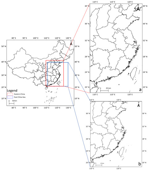
Figure 1.
The study area: (a) Eastern China; and (b) East China Sea.
Due to the limitations of Chinese SM observation data in time and space, we used GLDAS, developed by the National Oceanic and Atmospheric Administration (NOAA), National Environmental Prediction Center (NCEP), Goddard Space Flight Center (GSFC), and National Aeronautics and Space Administration (NASA). It is a combination of ground observation data with satellite data, having higher resolution and better results than other models. In the study, we applied the Noah model [17], which has high resolution and long time series. In addition, 0–10 cm monthly SM data, with the unit of kg/m2, were used in the study.
Cobe-SST data were collected from the Japan Meteorological Agency, with a resolution of 1° × 1° from 1891 to date, integrating the atmospheric dataset (International Comprehensive Ocean-Atmosphere Data Set, ICOADS), SST data, ship data, and buoy data by using the optimal interpolation method to mesh the grid. These data were also used in the JRA (The Japanese Reanalysis data) and the International Air Model Comparison Program (AMIP) experiment. It is one of the most commonly used data sets to describe SST [33]. Moreover, for the East China Sea region, Cobe-SST data incorporates enhanced observational data, which is more suitable than other data to describe the SST distribution off the Chinese coast [34].
Satellite-based AMSR-E SM and MODIS SST data were also used to compare with the results. AMSR-E SM data are provided by the national snow and ice center. The spatial resolution of level-3 land products (AE_Land3) was 1° × 1°, with the temporal resolution of monthly average. The time range was from 2004 to 2009. MODIS SST data are provided by Ocean Color. The L3 data of MODIS –Aqua satellite was used, with a spatial resolution of 4 km and a temporal resolution of monthly average ranging from 2004 to 2009 (see Table 1).

Table 1.
Basic data information.
SST and SM data were projected to regional average data from month to month, while the long-term change trend of the two datasets were filtered before attaining the change trend of the SSTA and SMA index. Then detrend data were processed into the standardization data.
2.2. Methods
We applied the methods such as detrending processing, z-score standardized processing, M-K trend test, regional correlation analysis, and time series causality analysis in the study.
2.2.1. Z-Score Standardized Processing
As the unit of each element is different, their average value and standard deviation are different. To compare them at the same level, a standardized method is used to make them a non-unit variable of the same level-a standardized variable for the weather element x and the data length n, the expression can be as follows:
where is the average value, and the average value is an estimate of the overall mathematical expectation of the element. The average (climate) condition of the element is reflected. is the mean square error, describing the average situation of the difference between the data and the average value in samples and reflecting the average variation degree of variables around average values (degree of discretization). The characteristics of data standardization are the average value of standardized variables as 0 and the variance of standardized variables is 1.
2.2.2. M-K Trend Test
The Manner–Kendall trend test is a statistical testing, usually applied to analyze the trend change of time series of climate factors such as precipitation, temperature and so on. It is widely used because of its simplicity and small interference. The specific method is a time series , and now calculates its test statistics S,
where the Sgn function is a step function that returns an integer that indicates the symbol of the specified number.
The method Var (S), can be obtained from the statistic S. Finally, the standard normal statistical variable Z can be obtained from S and Var (S).
The Z value indicates different trends. When z > 0, it means that the climate factor increases with time, whereas negative values are opposite. If you pass the significance test, it shows that the upward or downward trend is significant.
2.2.3. Regional Correlation Analysis
The correlation coefficient is the first statistical index designed by the statistician, Karl Pearson, and is the amount of linear correlation between study variables, generally indicated by the letter r. Because of the difference of research objects, the correlation coefficient has a variety of definitions, and the common correlation coefficient is the Pearson correlation coefficient. The correlation is a non-deterministic relationship, and the correlation coefficient is the amount of linear correlation between study variables. The simple correlated coefficient is the most widely used. It is the statistic that describes the linear correlation between the two variables. It is generally referred to as the correlation coefficient or the point correlation coefficient, expressed by r. It also serves as an estimate of the total coefficient of correlation. It is defined as:
There are several points worth paying attention to: (1) the correlation coefficient is the covariance of standardized variables; (2) −1 ≤ r ≤ 1; and (3) the larger the absolute value is, the closer the relationship between the variables is. When r > 0, the closer the two variables are to 1.0, the more significant the positive correlation is; when r < 0, the closer the two variables are, the closer the negative correlation is, the more significant the negative correlation is; when r ≤ 0, the two variables are independent of each other.
Whether the calculated correlation coefficient is significant or not needs to be tested for significance. The T test is generally used to test the significance of the correlation coefficient. Under the condition of the original assumption ρ = 0, the statistics are constructed as follows:
The statistic t obeys the t distribution with degree of freedom n ≤ 2. If you reject the original hypothesis, then reject the original hypothesis, or accept the original hypothesis. In this study, the confidence interval of 95% is 0.05, that is, 95% confidence interval. In fact, under the condition of fixed sample size, the correlation coefficient of the unified criterion can be calculated. If r > , the calculation process of is as follows:
2.2.4. Time Series Causality Analysis
Causality analysis is a method to predict things using the causality of the development and change of things. It is based on the causality of the development and change of things, grasp the relationship between the principal contradiction and the secondary contradiction, and establish a mathematical model to predict. In 1969, Granger proposed a statistical hypothesis test whose function is to determine whether a time series affects the prediction of another time series. The method is to calculate the errors and , if < , then the common prediction error of X and Y is less than that of X itself, that is, Y has Granger causality between X. The Granger causality method has been widely used in meteorology in recent years because of its simplicity and easy realization. Elsner et al. tested Granger causality with a global average near-surface temperature and Atlantic SST recorded during the Atlantic hurricane season. The results show that global near-surface temperatures can be used to predict Atlantic SST [35]. In terms of precipitation and SM, Salvucci et al. applied Granger causality to discuss the relationship between the two [36]. Although the Granger causality method has been successfully applied in many fields, it also has its limitations. Many researchers doubt the consistency between the Granger method and the real causality. In 2011, Hu et al. put forward a new theory of causality on the basis of determining the limitations of Granger causality. The causality between them is determined by the proportion of the contribution items of the time series of one variable to that of another variable to all the items. Su in the study of causality analysis and prediction of precipitation and SM, taking SM and precipitation as variables, the Granger method and the new causality method were compared, and the value in the meteorological field was affirmed [37]. In 2014, Liang proposed a new method to analyze causality based on the concept of information flow [38]. Causality in this method is measured by the time ratio of information flow from one sequence to another. For time series X1 and X2, the information flow rate from X2 to X1 is calculated. If is equal to zero, X2 does not cause X1. If is not equal to zero, then there is causality between X1 and X2. The specific process is shown in Figure 2.
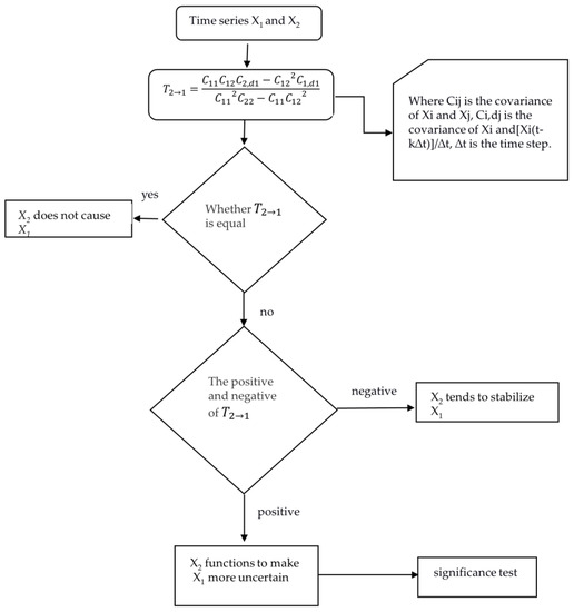
Figure 2.
Calculation flow chart of causality method based on information flow.
3. Results
3.1. The Evolutionary Characteristics of SM in EC and SST in the East China Sea
3.1.1. Long-Term Evolutionary Characteristics of Annual SST and SM
For this study, we selected 109–129°E, 18–40°N as the East China Sea search area, calculating regional average annual SST from 1961 to 2011 as shown in Figure 3 and Figure 4. Figure 3 shows the regional distribution of annual mean sea temperature, which in the East China Sea is between 12–26 °C, a figure that decreases with increase in latitude, taking into account the influence of solar radiation and land-sea distribution. In addition, the SST gradient nearshore area is larger than the open sea area. Figure 4 shows trends in annual average SST, which in the East China Sea presents a rolling rising trend peaking in 1998. At the same time, the Mann–Kendall test results show that the mean SST from 1961 to 2011 indicates a significant upward trend (slope of 0.01), with a ZC value of 4.0773. Figure 5 shows the annual mean SST anomaly sequence. Before 1987, SST negative anomalies were seen for 27 years and sea water was in a cold period, but after 1987 the SST has been warm on the whole.
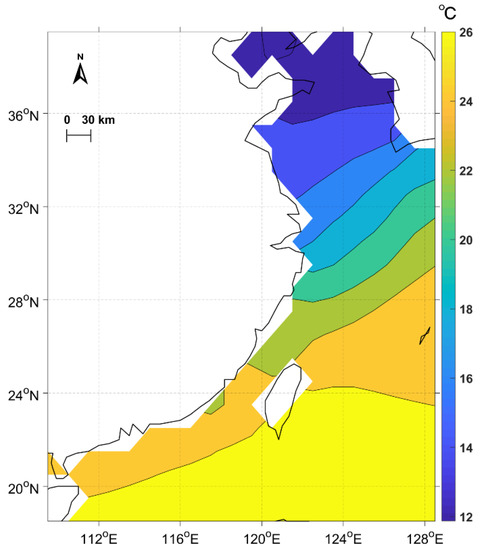
Figure 3.
Annual mean sea surface temperature (SST) distribution of the East China Sea from 1961–2011.
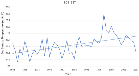
Figure 4.
Annual SST variation trend in the East China Sea from 1961–2011.
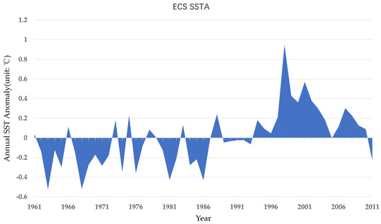
Figure 5.
Annual anomalies in SST (SSTA) variation trend in the East China Sea from 1961–2011.
We selected 108–124°E, 18–41°N as the study area for EC, calculating the regional average annual SM from 1961 to 2011, as shown in Figure 6 and Figure 7. Figure 6 shows the regional distribution of annual average SM, which in East Asia is between 8 and 35 kg/m2—generally high in the south and low in the north. Trend changes for average SM from 1961 to 2011 are shown in Figure 7. For all 51 years, SM in EC presents a rolling decreasing trend, peaking in 1964. At the same time, the Mann–Kendall test results show that mean SM from 1961 to 2011 exhibited a significant downward trend (slope of −0.01), with a ZC value of −3.0864. Analysis of anomalies in SM (SMA) from Figure 8 reveals that before 1978 SM was a long-term positive anomaly in the wet period; after 1978, SM was generally a negative anomaly in the dry period.
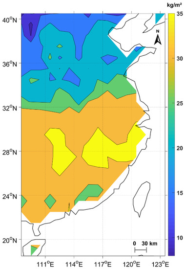
Figure 6.
Annual mean surface soil moisture (SM) distribution of the East China Sea from 1961–2011.
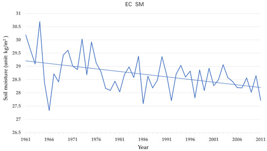
Figure 7.
Annual SM variation trend in the eastern China from 1961–2011.
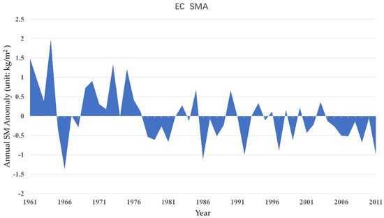
Figure 8.
Annual anomalies in SM (SMA) variation trend in the eastern China from 1961–2011.
3.1.2. Long-Term Evolutionary Characteristics of Seasonal SST and SM
Figure 9 shows the distribution of the average SST of the East China Sea in four seasons, which is generally consistent with the annual change. The SST range is 5–30 °C, from southwest to northeast overall, and is highest in summer and lowest in winter. SST in the Yellow Sea and Bohai Sea in spring and winter is significantly higher in the south than in the north. The temperature gradient in the East China Sea is obvious, with the temperature gradient greatest in autumn. The Mann–Kendall test was conducted on the SST for four seasons in the East China Sea, producing the results shown in Table 2. SST in all seasons showed an upward trend, among which the upward trend of SST in spring, autumn, and winter passed the significance test of 99%.
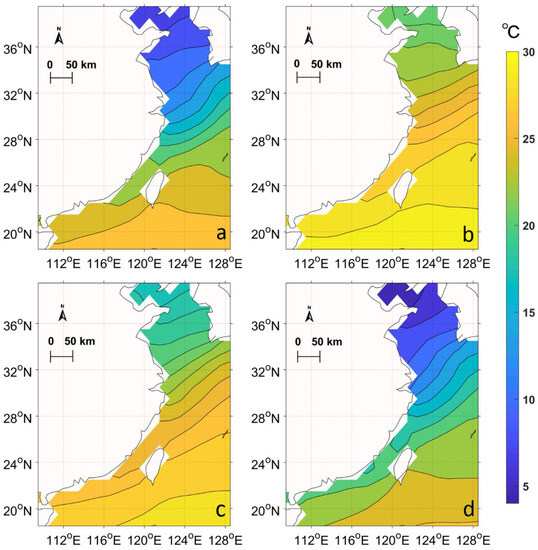
Figure 9.
Mean SST distribution during the four seasons of the East China Sea from 1961–2011: (a) spring; (b) summer; (c) autumn; and (d) winter.
Table 2.
Mann–Kendall trend test of annual mean sea surface temperature (SST) of four seasons.
Average SM distribution during the four seasons in eastern China is shown in Figure 10. The SM range is 5–40 kg/m2, which is generally higher in the south and lower in the north. SM in spring and winter in the north is significantly lower than in summer and autumn, whereas in the south changes in SM among the four seasons are relatively small, with SM remaining above 25 kg/m2. The trend of SM during the four seasons was tested, producing the results shown in Table 3. SM in each season showed a downward trend, with the downward trend of SM in spring and autumn passing the 99% significance test.
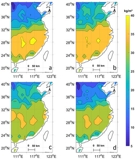
Figure 10.
Annual mean SM distribution of the East China Sea from 1961–2011. ((a) spring; (b) summer; (c) autumn;(d) winter.).
Table 3.
Mann–Kendall trend test of annual mean surface soil moisture (SM) of four seasons.
3.2. Analysis of SST in ECS and SM in EC
Many researchers have indicated that a range of key sea areas affects China’s summer precipitation, such as the eastern equatorial Pacific [39], the western Pacific warm pool [2], the Indian Ocean [40], the South China Sea [41], and the north Atlantic Ocean [42]. Combining certain authors’ studies on SM and precipitation, we averaged and standardized 51 years of regional SM data and monthly SST data and then calculated the regional correlation, finding that SST in the East China Sea is generally positively correlated with SM in eastern China and that correlation gradually decreases from south to north, among which the northern part of central China is weakly negatively correlated, as shown in Figure 11a. In addition, we used satellite data products to examine their correlation. Because satellite data starting times can differ significantly, we selected an overlapping time range. MODIS-SST data from 2004 to 2009 were averaged and standardized annually, after which regional correlation analysis was conducted with the SM of AMSR-E for the same time scale, as shown in Figure 11b. It can be seen that the general correlation distribution is basically consistent with the figure, exhibiting a positive–negative–positive distribution pattern from south to north. Because the time series of satellite data is relatively short, the value of the correlation coefficient is larger, among which the central China region, with its obvious differences, shows an opposite correlation. The area having the most consistent correlation was the coastal area of south China.
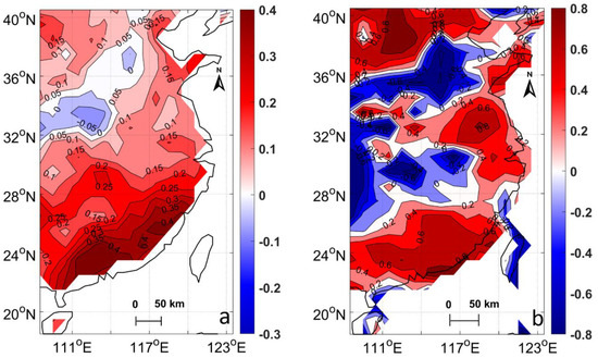
Figure 11.
Regional correlation analysis of SST and soil moisture in East China Sea. ((a) GLDAS-SM data and COBE-SST data); (b) AMSR-E SM data and MODIS-SST data).
The results of Figure 11a were tested for significance, with the coastal areas of south China found to be in the high-value area of positive correlation and to pass the 95% significance test—indicating that the SST anomaly of the East China Sea has the most significant effect on SM in the coastal areas of south China, with the highest correlation approaching 0.4, as shown in Figure 12. According to this finding, when the East China Sea is warm, SM in the southeast coastal areas generally shows positive anomalies, whereas when the East China Sea is cold, SM in the southeast coastal areas generally shows negative anomalies.
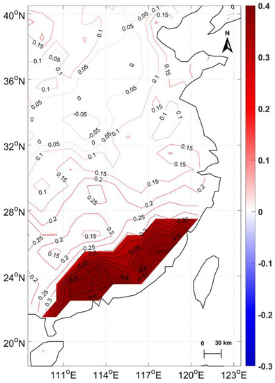
Figure 12.
Significant correlation between SST in the East China Sea and soil moisture in eastern China (passed 95% significance test).
3.2.1. Time-Lag Correlation and Time Series Causality Correlation between SST in ECS and SM in Significant Regions
Because SST in the East China Sea has the most significant effect on SM in the coastal areas of south China, these areas are considered to be significant areas; as a result, the correlation between SM in significant areas and SST in the East China Sea (ECS) has been further studied. The standardized linear trend of the average monthly SST data in the ECS and SM in significant regions were removed as shown in Figure 13. Before 1967, changes of SST and SM were in reverse phase, but from 1967 to 1997, they were in the same phase; since 1997, they have been in reverse phase again—perhaps because when the East China Sea is warm, the summer precipitation in the middle and lower reaches of the Yangtze River and the Huaihe River basin generally shows negative anomalies, whereas the summer precipitation in the coastal areas of Zhejiang, Fujian, and Guangdong in the south China, as well as in the south of northeast China, generally shows positive anomalies, thus affecting the anomaly of shallow SM, so that the two regions are abnormal. The degree of anomaly determines the overall SM state in eastern China.
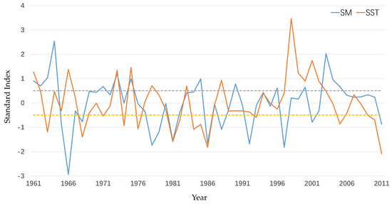
Figure 13.
The time series comparison of the 51-year average SST and SM after removing trend and standardizing.
Using Liang’s [38] time series causality theory to analyze SST and SM, we conclude that T12 and T21 are not equal to zero and that |T12| > |T21|, which means that the SST in ECS and the SM in significant regions have a causal relationship: both actively interact, but SST’s influence on SM is greater than SM’s influence on SST.
3.2.2. Seasonal Relationship between SST in ECS and SM in Significant Regions
The monthly average data for SM in coastal areas of south China, after removing trends and standardizing monthly average SST data in ECS, were analyzed season by season, as shown in Table 4.
Table 4.
Correlation analysis between the seasonal mean SST and SM from 1961 to 2011.
We can see from Table 4 that SM in spring is negatively correlated with SST in spring, summer, and winter, to a maximum of −0.98. SM in summer is positively correlated with SST in spring, summer, and winter, with a coefficient exceeding 0.80, but negatively correlated with SST in autumn, with a coefficient of −0.92. SM in autumn is negatively correlated with SST in spring and summer, reaching −0.96 before slightly decreasing to −0.78 in winter and positively correlating with SST in autumn, reaching 0.99. A strong positive correlation exists between SM in winter and SST in summer and winter, with a coefficient above 0.9. In conclusion, SM in spring and autumn shows a similar correlation with SST in four seasons, being positively correlated with SST in autumn and negatively correlated with SST in other seasons. SM in summer and winter correlated with SST in the four seasons, contradicting the foregoing conclusions.
Rises in SST are known to alter sea and air fluxes, such as the sensible heat and latent heat at the sea surface, and cause changes in atmospheric convection over the region, altering local atmospheric circulation. The research shows that the prediction results of SM can be significantly improved by including SST as an external force. In the tropics SST improves the predictability of local SM, mainly by affecting surface temperature and precipitation. In other regions, SST’s influence on wind speed, cloud cover, and surface evaporation also plays an important role in improving the predictability of SM [43]. Both the coastal areas of south China and the East China Sea are in the East Asian monsoon area, and thermal variations in the East China Sea will inevitably cause changes in the underlying surface energy and water of the east Asian monsoon circulation [5]. The anomaly of the east Asian summer monsoon often leads to severe drought and floods in China, whereas the anomaly of the winter monsoon causes severe weather disasters such as cold, rain, and snow. Table 4 shows that the correlation is greatest between SST [44,45,46] and SM in winter and summer. Accordingly, it can be speculated that the seasonal differences in the correlation between SM in the coastal areas of south China and SST in the East China Sea are related mostly to monsoon circulation—although the underlying mechanism still requires further study.
4. Discussion
SST and SM in EC generally showed the opposite trends over past 51 years. From the perspective of correlation, the interannual changes of the two are owerall positively correlated, whereas the seasonal cjanges are different to some extent. SM in spring and autumn shows a similar correlation with SST in the four season, so that SM in spring and autumn is positively correlated with SST in autumn and negatively with SST in other seasons. SM in summer and winter was correlated with SST in the four seasons, contradicting the foregoing conclusions. This finding may suggest that the seasonal differences in the correlation between SM and SST are related mostly to monsoon circulation.
The correlation between SM in EC and SST in the East China Sea was confirmed by our causal analysis, but we found that not only SST in the East China Sea but also the SST anomaly in the El Nino area may cause atmospheric circulation anomalies that affect precipitation and SM anomalies in EC.
Abnormal SST affects SM, and SM in turn affects climate, leading to changes in SST. However, the climate is also affected by other external forces, so that the extent to which SM, rather than external forces, affects SST remains unclear.
Up to now, we have studied only offshore SST and SM in eastern China, considering a significant related area that is in the southeast coastal area. Future research will expand the scope of the sea area, seeking areas that are more sensitive to the influence of SM in China.
In this study, the correlation between SST and SM was analyzed quantitatively, but its internal mechanism was not considered. In subsequent studies, we will analyze the physical and thermodynamic mechanisms between the two, seeking deeper understandings of the climatic effects of SM.
In addition, in view of SST’s influence on SM, our next study will focus on whether including SST as a factor in SM prediction will improve the fitting accuracy and prediction accuracy of regression equations.
5. Conclusions
From the perspective of the long time series, SST in the East China Sea shows a warming trend, especially since 1987. SM in EC shows a drying trend obvious after 1978. The seasonal average distribution and annual average distribution of SST are essentially the same, increasing in the northwest and southeast, and SST in spring, autumn, and winter shows a significant upward trend. The seasonal average distribution of SM is higher in the south and lower in the north, and SM in spring and autumn shows a significant downward trend.
Regional correlation analysis reveals that the most important related area is the southeast coastal area. The connection between SST and SM has seldom been discussed by scholars, but based on Liang’s time series causality analysis, we can find that SM in EC is related to SST in the East China Sea, as well as that SST has more influence on SM than vice versa.
According to correlation analysis between the seasonal mean SST and SM from 1961 to 2011, SM in spring and autumn shows a similar correlation with SST in the four seasons, so that SM in spring and autumn is positively correlated with SST in autumn and negatively correlated with SST in other seasons. SM in summer and winter was correlated with SST in the four seasons, contradicting the foregoing conclusions.
In summary, the seasonal and regional changes to the thermodynamic state of the East China Sea will affect the trend of SM in EC.
Author Contributions
Conceptualization, Y.Z. and J.C.; methodology, Y.L.; software, J.C.; validation, Y.L., J.C., and Y.Z.; formal analysis, Y.L.; investigation, J.C.; resources, Y.Z., J.Y.T.; data curation, Y.L.; writing—original draft preparation, Y.L.; writing—review and editing, Y.Z., J.Y.T.; visualization, Y.L.; supervision, Y.Z.; project administration, Y.Z. All authors have read and agreed to the published version of the manuscript.
Funding
This research was funded by the National Natural Science Foundation (U1901215), the Natural Scientific Foundation of Jiangsu Province (BK20181413), and the National Key Research and Development Program of China (Project Ref. No. 2016YFC1402003).
Acknowledgments
GLDAS data, AMSR-E SM data, and MODIS SST data are highly appreciated in this study. AMSR-E data was provided by NEESPI Data Center Project (2002), AMSR-E/Aqua level 3 global monthly Surface Soil Moisture Averages V005, Greenbelt, MD, USA, Goddard Earth Sciences Data and Information Services Center(GES DISC), Accessed: 2019/12/29, https://disc.gsfc.nasa.gov/datacollection/AMSRE_AVRMO_005.html. MODIS SST data was provided by NASA Goddard Space Flight Center, Ocean Ecology Laboratory, Ocean Biology Processing Group; (2014): Sea-viewing Wide Field-of-view Sensor (SeaWiFS) Ocean Color Data, NASA OB. DAAC. doi:10.5067/ORBVIEW-2/SEAWIFS_OC.2014.0. Accessed on 29 December 2019. We also thank the joint support from the National Natural Science Foundation (U1901215), the Natural Scientific Foundation of Jiangsu Province (BK20181413), and the National Key Research and Development Program of China (Project Ref. No. 2016YFC1402003).
Conflicts of Interest
The authors declare no conflict of interest.
References
- Cai, J.Z.; Zhang, Y.Z.; Li, Y. Analyzing the Characteristics of Soil Moisture Using GLDAS Data: A Case Study in Eastern China. Appl. Sci. 2017, 7, 566. [Google Scholar] [CrossRef]
- Huang, R.H.; Sun, F.Y. Impacts of Thermal State and the Convective Activities in the Tropical Western Warm Pool on the Summer Climate Anomalies in East China. Sci. Atmos. Sin. 1994, 18, 141–151. [Google Scholar]
- Cai, R.S.; Chen, J.L.; Huang, R.H. The Response of Marine Environment in the Offshore Area of China and Its Adjacent Ocean to Recent Global Climate Change. Chin. J. Atmos. Sci. 2006, 30, 1019–1033. [Google Scholar]
- Cai, R.S.; Tan, H.J. Influence of interdecada climate variation over East Asia on offshore ecopgical system of China. J. Oceanogr. Taiwan 2010, 29, 173–183. [Google Scholar]
- Li, C.H.; Cai, R.S.; Chen, J.L. Temporal and Spatial Characteristics of Latent Heat Flux in the East China Sea and Its Association with Summer Rainfall in East China. Plateau Meteorol. 2010, 29, 1485–1492. [Google Scholar]
- Liang, P.; Ding, Y.H.; He, J.H. Relations Between Summer Rainfall over the Lower Reach of Yangtze River and East Asian Summer Monsoon as well as Sea Surface Temperature over the Pacific in Spring. Plateau Meteorol. 2008, 27, 772–777. [Google Scholar]
- Sun, Y.; Wang, Q.Q.; Qian, Y.F. Relation between the Summer Rainfall Anomalies in North China and the Global SSTA. Plateau Meteorol. 2006, 25, 1127–1138. [Google Scholar]
- Wen, X.F.; Zhang, Q.L.; Yang, Y.L. The Kuroshio Heat Transport in the East China Sea and its Relation to the Orecipitation in the Rainy Season in the Huanghai Plain Area. Oceanol. Limnol. Sin. 1996, 27, 237–245. [Google Scholar]
- Zhang, T.Y.; Sun, Z.B.; Li, Z.X. Relation between spring kuroshio ssta and summer rainfall in china. J. Trop. Meteorol. 2007, 13, 165–168. [Google Scholar]
- Robock, A.; Vinnikov, K.Y.; Srinivasan, G. The global soil moisture data bank. Bull. Am. Meteorol. Soc. 2000, 81, 1281. [Google Scholar] [CrossRef]
- Guo, N.; Chen, T.Y.; Lei, J.Q. Estimating Farmland Soil Moisture in Eastern Gansu Province Using Noaa Satellite Data. J. Appl. Meteorol. Sci. 1997, 8, 212–218. [Google Scholar]
- Zhang, Q.; Qiao, F.J.; Niu, H.S. Sensitivity Analysis of Soil Moisture to Vegetation Index in North China. Chin. J. Ecol. 2005, 24, 715–718. [Google Scholar]
- Manabe, S. Climate and the Ocean Circulation 1. Mon. Weather Rev. 1969, 97, 806–827. [Google Scholar]
- Dickinson, R.E.; Henderson-Sellers, A.; Kennedy, J. Biosphere Atmosphere Transfer Scheme (BATS). In Encyclopedia of Hydrological Sciences; American Cancer Society: Atlanta, GA, USA, 2006. [Google Scholar]
- Sellers, P.J.; Mintz, Y.; Sud, Y.C. A Simple Biosphere Model (SIB) for Use within General Circulation Models. J. Atmos. Sci. 1986, 43, 505–531. [Google Scholar] [CrossRef]
- Dai, Y.; Zeng, X.; Dickinson, R.E. The Common Land Model. Bull. Am. Meteorol. Soc. 2003, 84, 1013–1023. [Google Scholar] [CrossRef]
- Rodell, M.; Houser, P.R.; Jambor, U. The global land data assimilation system. Bull. Am. Meteorol. Soc. 2004, 85, 381–394. [Google Scholar] [CrossRef]
- Guo, C.J.; Chen, H.S.; Xu, P. Possible Relationship Among South China Sea SSTA, Soil Moisture Anomalies in Southwest China and Summer Precipitation in Eastern China. J. Trop. Meteorol. 2013, 29, 75–82. [Google Scholar]
- Chen, J.L.; Sun, X.G.; Tang, H.S. Comparative analysis of soil moisture observations and reanalysis in Jiangsu Province. J. Meteorol. Sci. 2018, 38, 105–112. [Google Scholar]
- Zhu, Z.; Shi, C.X.; Zhang, T. Applicability Analysis of Four Soil Moisture Reanalysis Datasets in China. Plateau Meteorol. 2018, 37, 240–252. [Google Scholar]
- Ma, S.Y.; Zhu, K.W.; Li, M.X. A Comparative Study of Multi-source Soil Moisture Data for China’s Regions. Clim. Environ. Res. 2016, 21, 121–133. [Google Scholar]
- Cui, Y.Y.; Jing, W.Q.; Qin, J. Applicability Evaluation of Merged Soil Moisture in GLDAS-NOAH and CLDAS-V2.0 Products over Qinghai—Tibetan Plateau of 2015 Based on TIPEX Ⅲ Observations. Plateau Meteorol. 2018, 37, 4–21. [Google Scholar]
- Ghazanfari, S.; Pande, S.; Hashemy, M. Diagnosis of GLDAS LSM based aridity index and dryland identification. J. Environ. Manag. 2013, 119, 162–172. [Google Scholar] [CrossRef]
- Spennemann, P.C.; Rivera, J.A.; Saulo, A.C. A Comparison of GLDAS Soil Moisture Anomalies against Standardized Precipitation Index and Multisatellite Estimations over South America. J. Hydrometeorol. 2015, 16, 158–171. [Google Scholar] [CrossRef]
- Niu, G.Y.; Yang, Z.L.; Dickinson, R.E. Development of a simple groundwater model for use in climate models and evaluation with Gravity Recovery and Climate Experiment data. J. Geophys. Res. Atmos. 2007, 112. [Google Scholar] [CrossRef]
- Quintana-Seguí, P.; Le Moigne, P.; Durand, Y. Analysis of near-surface atmospheric variables: Validation of the SAFRAN analysis over France. J. Appl. Meteorol. Climatol. 2008, 47, 92–107. [Google Scholar] [CrossRef]
- Reichle, R.H.; Koster, R.D.; Liu, P. Comparison and assimilation of global soil moisture retrievals from the Advanced Microwave Scanning Radiometer for the Earth Observing System (AMSR-E) and the Scanning Multichannel Microwave Radiometer (SMMR). J. Geophys. Res. Atmos. 2007, 112. [Google Scholar] [CrossRef]
- Liu, L.W.; Wei, D.; Wang, X.W. Multi-data Intercomparison of Soil Moisture over China. J. Arid. Meteorol. 2019, 37, 40–47. [Google Scholar]
- Koster, R.D.; Dirmeyer, P.A.; Guo, Z. Regions of strong coupling between soil moisture and precipitation. Science 2004, 305, 1138–1140. [Google Scholar] [CrossRef]
- Hu, Y.M.; Ding, Y.H.; Liao, F. An improvement on summer regional climate simulation over East China: Importance of data assimilation of soil moisture. Chin. Sci. Bull. 2009, 54, 2388–2394. [Google Scholar] [CrossRef]
- Zhang, X.Z.; Wu, X.Y.; He, J.H. Vertical Character of Soil Moisture in China. Acta Meteorol. Sin. 2004, 62, 60. [Google Scholar]
- Ma, Z.G.; Wei, H.L.; Fu, Z.B. Relationship Between Regional Soil Moisture Variation and Climatic Variablity Over East China. Acta Meteorol. Sin. 2000, 58, 284–286. [Google Scholar]
- Li, S.; Guo, J.R.; Jiang, X.Y. Sources and analysis of multi-temporal-spatial scale marine hydrometeology data. Mar. Sci. Bull. 2020, 39, 24–39. [Google Scholar]
- Tan, H.J.; Cai, R.S.; Huang, R.H. Enhanced Responses of Sea Surface Temperature over Offshore China to Global Warming and Hiatus. Clim. Chang. Res. 2016, 12, 500–507. [Google Scholar]
- Elsner, J.B. Evidence in support of the climate change–Atlantic hurricane hypothesis. Geophys. Res. Lett. 2006, 33, L16705. [Google Scholar] [CrossRef]
- Salvucci, G.D.; Saleem, J.A.; Kaufmann, R. Investigating soil moisture feedbacks on precipitation with tests of Granger causality. Adv. Water Resour. 2002, 25, 1305–1312. [Google Scholar] [CrossRef]
- Su, H. Causality Analysis among Precipitation, Soil Moisture and Precipitation Prediction. Master’s Thesis, Hangzhou Electrical University, Hangzhou, China, 2018. [Google Scholar]
- Liang, X.S. Unraveling the cause-effect relation between time series. Phys. Rev. E 2014, 90, 052150. [Google Scholar] [CrossRef]
- Chen, L.T.; Wu, R.G. The Joint Effects of SST Anomalies over Different Pacific Regions on Summer Rainbelt Patterns in Eastern China. Sci. Atmos. Sin. 1998, 22, 718–726. [Google Scholar]
- Chen, L.T. Zonal anomaly of sea surface temperature in the tropical Indo-Pacific Ocean and its effect on summer Asia monsoon. Chin. J. Atmos. Sci. 1988, 12, 142–148. [Google Scholar]
- Zhang, Q.; Liu, P.; Wu, G.X. The Relationship between the Flood and Drought over the Lower Reach of the Yangtze River Valley and the SST over the Indian Ocean and the South China Sea. Chin. J. Atmos. Sci. 2003, 27, 992–1006. [Google Scholar]
- Xu, H.M.; He, J.H.; Dong, M. Interannual Variability of the Meiyu Onset and its Association with North Atlantic Oscillation and SSTA over North Atlatic. Acta Meteorol. Sin. 2001, 59, 694–706. [Google Scholar]
- Zhu, S.G.; Chen, H.S.; Dong, X.; Wei, J.F. Infuence of persistence and oceanic forcing on global soil moisture predictability. Clim. Dyn. 2020, 54, 3375–3385. [Google Scholar] [CrossRef]
- Ji, C.X.; Zhang, Y.Z.; Cheng, Q.M. Analyzing the variation of the precipitation of coastal areas of eastern China and its association with sea surface temperature (SST) of other seas. Atmos. Res. 2019, 219, 114–122. [Google Scholar] [CrossRef]
- Zhang, Y.Z.; Huang, Z.J.; Fu, D.Y. Monitoring of chlorophyll-a and sea surface silicate concentrations in south part of Cheju island in the East China sea using MODIS data. Int. J. Appl. Earth Obs. Geoinf. 2018, 67, 173–178. [Google Scholar] [CrossRef]
- Ji, C.X.; Zhang, Y.Z.; Cheng, Q.M. Evaluating the impact of sea surface temperature (SST) on spatial distribution of chlorophyll-a concentration in the East China Sea. Int. J. Appl. Earth Obs. Geoinf. 2018, 68, 252–261. [Google Scholar] [CrossRef]
© 2020 by the authors. Licensee MDPI, Basel, Switzerland. This article is an open access article distributed under the terms and conditions of the Creative Commons Attribution (CC BY) license (http://creativecommons.org/licenses/by/4.0/).