Abstract
Based on 26 years of satellite altimetry, this study reveals the presence of a persistent east–west pattern in the sea level of the Red Sea, which is visible throughout the years when considering the east–west difference in sea level. This eastern–western (EW) difference is positive during winter when a higher sea level is observed at the eastern coast of the Red Sea and the opposite occurs during summer. May and October are transition months that show a mixed pattern in the sea level difference. The EW difference in the southern Red Sea has a slightly higher range compared to that of the northern region during summer, by an average of 0.2 cm. Wavelet analysis shows a significant annual cycle along with other signals of lower magnitude for both the northern and southern Red Sea. Removing the annual cycle reveals two energy peaks with periodicities of <12 months and 3–7 years, representing the intraseasonal and El Nino—Southern Oscillation (ENSO) signals, respectively. Empirical Orthogonal Function (EOF) analysis shows that EOF1 corresponds to 98% of total variability, EOF2 to 1.3%, and EOF3 to 0.4%. The remote response of ENSO is evident in the variability in the atmospheric bridge, while that of the Indian Ocean Dipole (IOD) and North Atlantic Oscillation (NAO) is weak. Three physical mechanisms are responsible for the occurrence of this EW difference phenomenon, namely wind, buoyancy, and the polarity of eddies.
1. Introduction
Sea level is a crucial climate indicator that has been widely studied both globally and regionally [1,2,3] and has played a vital component in understanding the dynamics of the upper layer of the ocean [4,5]. A small-scale change in sea level may have an adverse impact on the physical and biological processes of such regions, and therefore it is vital to properly understand the spatial and temporal variability in sea level [6,7].
The Red Sea is an important marginal sea known for unique oceanographic characteristics and complex distinctive marine ecosystems. It supports the high diversity of corals and holds precious repositories of marine biodiversity [8]. The Red Sea is located between the African and Asian continents (12–30°N & 32–44°N), oriented from north–northwest (NNW) to south–southeast (SSE). It is a semi-enclosed basin, with a length of about 2000 km, an average width of 280 km and an average depth of about 500 m [9]. The sea level variability in the Red Sea is mainly influenced by the exchange between the Red Sea and the Gulf of Aden, which is primarily driven by thermohaline effect and the seasonally reversing wind regime in the Red Sea [10,11,12,13,14,15].
The Red Sea is characterized by a strong evaporation rate of about 2 m·1yr−1 [16], with nearly zero precipitation, and is known as one of the hottest and most saline regions in the world. The wind pattern in the Red Sea is characterized by seasonal and regional differences in both speed and direction. However, the predominant direction of the wind in the northern Red Sea is from the NNW throughout the year while that in the southern Red Sea is from the SSE during winter and from the NNW during summer [16,17].
The surface current flow is in the southward direction during summer and in the northward direction during winter. During summer, the buoyancy flux is positive in the northern Red Sea and negative in the southern Red Sea, leading to a southward buoyancy/density gradient flow. Moreover, the predominant wind is from NNW during this period. The buoyancy gradient and the wind drag together result in a southward flow during summer. During winter, the buoyancy gradient reverses to negative buoyancy in the northern Red Sea and positive buoyancy in the southern Red Sea. Apart from this, the wind in the southern Red Sea reverses its direction to blow from SSE, while northern Red Sea winds become weaker. The reverse buoyancy gradient and changes in the wind collectively generate a northward current during winter [9,17,18].
The availability of satellite altimetry records for more than two and half decades have provided an unprecedented opportunity to better understand the spatial and temporal variability in sea level. In recent years, an increasing interest has been observed in altimetry-based sea level studies globally and regionally [2,3,19,20,21,22,23]. However, relatively less attention is paid to the Red Sea in comparison to other regions of the world. As stated in previous studies, the Red Sea is characterized by a high sea level during winter and a low sea level during summer [9,11,17,24,25]. Noticeably, most of the studies were based on data for a short period or using the point observations from tidal stations. Some recent studies have investigated the long-term sea level variability using altimetry and discussed the geostrophic current [20], and the impact of tropical climate modes on the sea level [19,26].
The main objective of the present study is to explore the 26-year long satellite altimetry record to further understand the spatial and temporal variability of the sea level in the Red Sea. We have identified a permanent east–west pattern of sea level variability between the eastern and western Red Sea, in addition to the previously reported seasonal and interannual cycles [11,12,14,17,20,24,26,27]. This paper discusses the spatial and temporal variability of this observed east–west sea level pattern based on the satellite altimetry record during the 1993–2018 period. The rest of the paper is arranged as follows: Section 2 describes the data sets used and the method of analysis applied; the results from the present study are included in Section 3; the dynamics of sea level variability are discussed in Section 4, and the conclusions are summarized in the final section.
2. Materials and Methods
2.1. Data
Sea level anomaly (SLA) maps are available from the Copernicus Marine environment monitoring service (http://marine.copernicus.eu/services-portfolio/access-to-products), which were previously provided by Archiving, Validation, and Interpretation of Satellite Oceanographic data (AVISO) from 1993 to present. The SLA is prepared by merging the data from altimetry missions Envisat, Jason-1, Jason-2, Jason-3, ERS-1, ERS-2, GFO, Topex/Poseidon, Cryosat-2, Saral/AltiKa, HY-2A, and Sentinel 3A. The reanalysis products are considered to be more precise compared to the near-real-time (NRT) products but have a delay of few months (data available up to 13 May 2019 while doing this analysis) in becoming publicly available. In the present study, the reanalysis of delayed-time gridded SLA is used for the period from 1 Jan 1993 to 31 Dec 2018, with a spatial resolution of 0.25° × 0.25° and a temporal resolution of one day.
The wind data is taken from the National Centers for Environmental Prediction (NCEP)’s Climate Forecast System Reanalysis (CFSR, https://rda.ucar.edu/datasets/ds093.1/?hash=!access) available during the period 1993–2010 and from Climate Forecast System (CFSv2, an upgraded product of CFSR, https://rda.ucar.edu/datasets/ds094.1/) available during the period 2010–2018. The temporal resolution of wind data for both CFSR and CFSv2 is the same (hourly), while the spatial resolution is slightly different (0.312° × 0.312° for CFSR and 0.2° × 0.2° for CFSv2). Therefore, the data are re-gridded to 0.25° × 0.25° (similar to that of SLA) using bilinear interpolation.
The climate indices data corresponding to climate modes ENSO (El-Nino Southern Oscillation), IOD (Indian Ocean Dipole), and NAO (North Atlantic Oscillation) [28,29,30] are downloaded from the following sources: Multivariate ENSO Index Version 2 (MEI V2, https://www.esrl.noaa.gov/psd/data/correlation/meiv2.data), Dipole Mode Index (DMI, https://www.esrl.noaa.gov/psd/gcos_wgsp/Timeseries/DMI/), and North Atlantic Oscillation (NAO, https://www.esrl.noaa.gov/psd/data/correlation/nao.data).
2.2. Methods
The Red Sea is classified into the eastern and western Red Sea, as shown in Figure 1. The black line in Figure 1 passes through the approximate middle of the Red Sea basin, and the portions of the basin to the east and west are named the eastern and western Red Sea, respectively. The eastern–western (EW) difference is estimated for every 0.25° interval along the latitude by taking the difference in mean SLA for both eastern and western sides. In the case of the coastal grid point, the difference is estimated by considering the most eastern and western grid points. The long-term analysis of SLA and wind datasets is carried out using the freely available scientific processing tool climate data operator (CDO, https://code.mpimet.mpg.de/projects/cdo/).
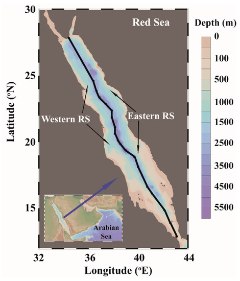
Figure 1.
The geographical location and the bathymetry of the study area. The eastern and western Red Sea is marked and is separated using an axial line (black line) passing through the approximate middle of the Red Sea.
The season in the Red Sea is classified based on the mean monthly wind pattern in the basin. November to March is considered winter, during which the SSE wind prevails in the southern Red Sea and NNW winds prevail in the northern Red Sea. June to September is considered the summer, where the wind in the entire basin blows NNW and relatively stronger than in winter. The months April-May and October are, respectively, considered the spring and autumn seasons.
3. Results
The spatial and temporal variability of the sea level in the Red Sea is analyzed based on satellite altimetry records for the period from 1993 to 2018. Apart from the previously documented findings [11,17,19], the analysis has shown an interesting pattern of the east–west difference in the sea level between the eastern and western sides of the Red Sea, which is seen in all years and has significant seasonal variability. The spatial and temporal variability of this east–west difference (hereafter “EW difference”) is investigated to understand the short-term and long-term variability based on SLA derived from satellite altimetry records from 1993 to 2018 (26 years).
The temporal variability of the EW difference for two coastal data points from the eastern and the western parts of the Red Sea at 26°N (an arbitrary location) is shown in Figure 2a. Instances of positive and negative values are observed at regular intervals of approximately 12 months. A positive value of the EW difference indicates that the sea level at the eastern side of the Red Sea is higher than that of the western side. To minimize the noise in the signal, we averaged the EW difference for the entire basin and show it in Figure 2b. From the figures, it is clear that a significant seasonal cycle exists in the variability of the EW difference in the Red Sea.
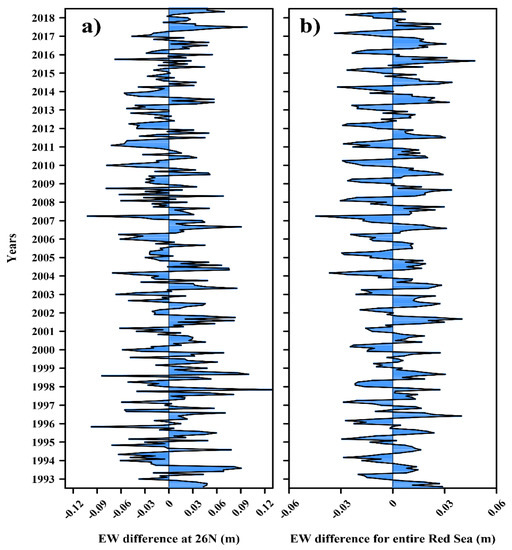
Figure 2.
(a) The monthly mean eastern–western (EW) difference between the most easterly and most westerly grid points at 26°N (longitude values are 36.625°E and 34.375°E respectively). (b) The monthly mean EW difference between the eastern and the western half of the Red Sea.
The monthly climatology of EW difference is prepared for each latitude for every 0.25°, which shows that the EW difference exists from the north to the south of the Red Sea (Figure 3a,b). We considered the region between 15°N & 27°N to remove the Gulf of Suez, the Gulf of Aqaba, and the Bab al Mandab strait from the calculation. The climatology shows that the sea level in the eastern Red Sea is clearly higher than that of the western region during January and February in the entire basin, but the pattern exists in at least 70% of the basin from November to April. Similarly, the western side is visibly higher than the eastern side from July to September. The months of May–June and October display a mixed pattern of the EW differences. In both transition periods, winter to summer and summer to winter, the reversal was first observed in the northern Red Sea. We have also noticed that the summer peak of the sea level in the western region is slightly higher (0.3 cm on average) than that of winter peak in the eastern region.
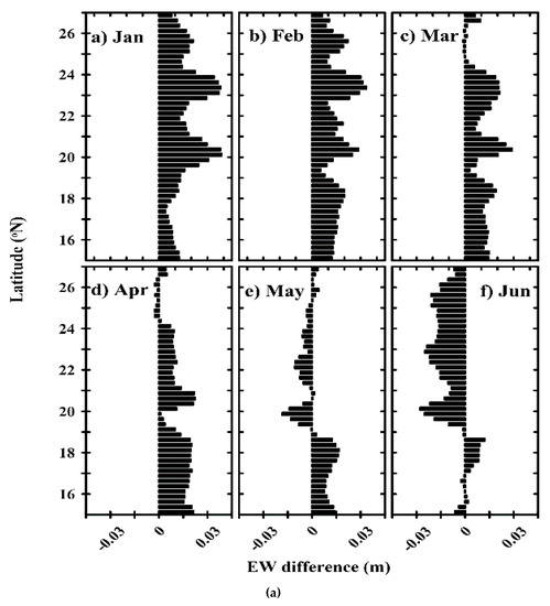
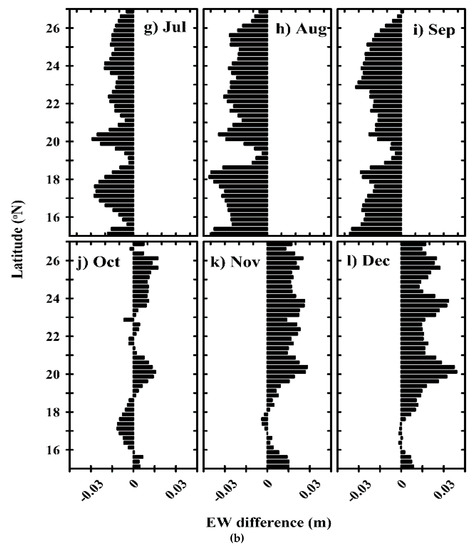
Figure 3.
Monthly climatology of EW difference in sea level for different latitudes (a) from January to June and (b) from July to December.
The mean patterns of winter and summer EW difference (Figure 4) are clearly opposite, while the spring and autumn seasons have a mixed pattern (figure not shown). The higher sea level observed in the eastern side of the Red Sea during winter shifts to the western side during summer.
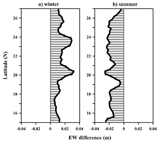
Figure 4.
The mean EW difference during (a) winter and (b) summer.
Since the Red Sea region is geographically located in an inclined plane with the imaginary axial line tilted by ~32 degrees in the anti-clockwise direction with respect to the meridian, we have also repeated the analysis by considering the inclination of the axis. To consider this aspect in the analysis, we have considered the eastern and western regions using boxes in an inclined plane (32 degrees tilted toward left) as shown in Figure 5.
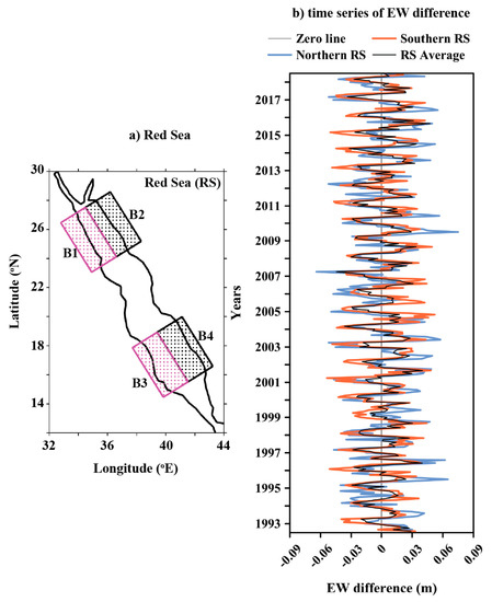
Figure 5.
(a) The rectangular boxes considered from the northern and southern Red Sea in an inclined plane (inclined to the left by 32 degrees from true north). The boxes are named B1 (northwestern), B2 (northeastern), B3 (southwestern), and B4 (southeastern). (b) The time series of the EW sea level difference for the northern (B2-B1) and southern (B4-B3) basin.
The EW differences are estimated for the data points that fall into the boxes named B1 (northwestern), B2 (northeastern), B3 (southwestern), and B4 (southeastern), as shown in Figure 5a. The EW difference in sea level for the northern and southern Red Sea is shown in Figure 5b. The variability in both the northern and southern Red Sea are in phase; however, a small difference can be observed in the amplitude of variability.
A wavelet analysis is applied to the average EW difference for the northern and southern Red Sea to identify temporal frequencies in the signal (Figure 6). The result shows the presence of a significant annual cycle for both the northern and southern Red Sea, along with other signals of relatively small magnitudes.
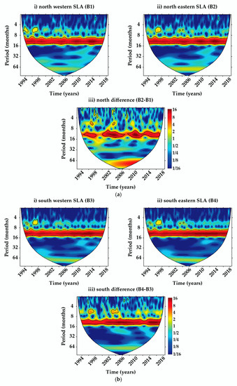
Figure 6.
The wavelet plots for the western basin, eastern basin, and their difference (a) for the northern Red Sea and (b) for the southern Red Sea.
To quantify the contribution of different signals to sea level, EOF analysis is carried out (figure not shown). The first three EOF modes together account for nearly all of total variations in sea level in the Red Sea. The fist mode predominantly explains about 98% of the total variation and mainly represents the annual component, while the second (1.3%) and third (0.4%) modes of variability are negligibly small. This is in agreement with previous studies [14,24], which have shown that the annual cycle is dominating the sea level variability of the Red Sea.
The wavelet analysis is repeated after removing the annual signal from the time series (Figure 7), which shows the presence of two additional energy peaks for most of the data period, with periodicities <12 months and 3–7 years representing the intra-seasonal and ENSO signals, respectively [19,31].
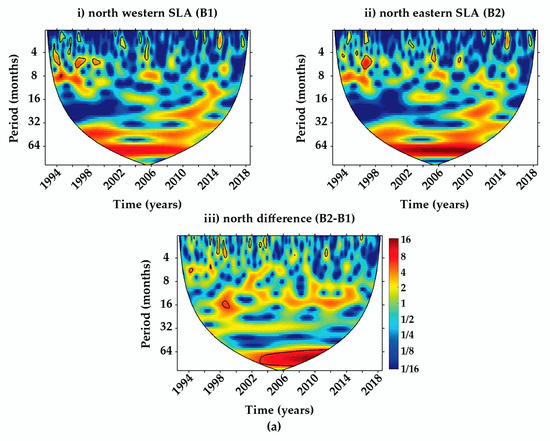
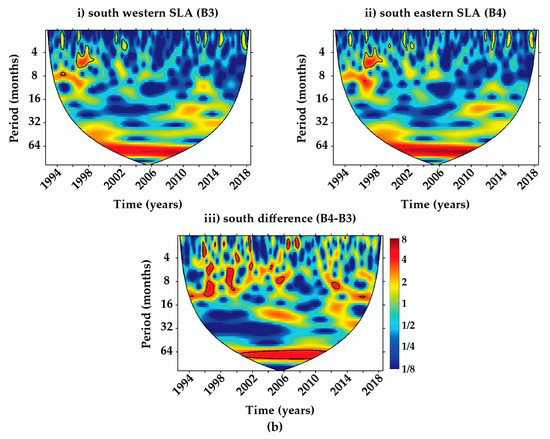
Figure 7.
The wavelet plots after removing the annual signals for the western basin, eastern basin, and their difference (a) for the northern Red Sea and (b) for the southern Red Sea.
In brief, a significant seasonally reversing EW difference pattern exists in the Red Sea. The average annual cycle of EW difference for the northern, southern, and whole basin of the Red Sea is shown in Figure 8. On average, the eastern side is higher than the western side from November to March and vice versa from June to September (Figure 8), indicating that the eastern side has a higher sea level for a period twice as long (8 months) as the western side (4 months).
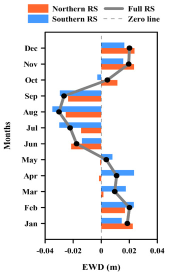
Figure 8.
The EW difference pattern for the northern Red Sea (orange), the southern Red Sea (blue), and the whole Red Sea basin (grey).
The characteristics of eddies in the Red Sea are also analyzed, as the polarity of eddies (cyclonic or anticyclonic) can significantly influence the spatial sea level difference in narrow basins like that of the Red Sea. The eddies were mostly concentrated in the central and northern Red Sea compared to the southern region. The number of cyclonic eddies was relatively larger than of anticyclonic eddies. The relative dominance of cyclonic eddies is observed in the western Red Sea during winter, which more or less shifts to the eastern side during summer [20]. This can result in relatively lower sea level regions in the western Red Sea during winter and in the eastern Red Sea during summer.
The relation of the observed EW difference in sea level with climate events such as the El Nino—Southern Oscillation (Multivariate ENSO Index V2, MEI), Indian Ocean Dipole (Dipole Mode Index, DMI), and North Atlantic Oscillation (NAO index) are investigated to explore the possibility of the remote response of these events in the Red Sea. The EW difference in sea level is positively related to MEI throughout the year, with maximum correlation during spring and autumn seasons (with correlation coefficients of 0.44 and 0.51, respectively. The correlation values during winter and summer are also positive but are not statistically significant.
No significant relation is observed between the EW difference and DMI in the Red Sea. The previous study also reported similar results [26], that there is only a weak relation between sea level and DMI in the Red Sea. Similarly, the analysis also shows that the relation between NAO and EW difference is weak throughout the year, indicating the absence of any significant influence of the EW difference on the sea level. This result is consistent with previous studies [19,26]. In brief, MEI (or ENSO) is observed to be the dominant remote force influencing the EW difference in the sea level of the Red Sea.
4. Discussion
Different parameters were analyzed to understand the ongoing dynamics in the Red Sea, which led to the observed EW difference pattern, where relatively higher sea levels are observed in the eastern Red Sea during winter and in the western Red Sea during summer.
During winter, the northward density gradient and the relatively strong SSE winds (>7 m/s) in the southern Red Sea drive a mean northward current in the surface layer. During this period, a relatively weak NNW wind prevails in the northern Red Sea (<4 m/s), which is in the opposite direction of the surface current flow [16,24]. However, the current continues its northward flow, mostly overcoming the relatively weak wind in the opposite direction. The northward current results in a pile-up of water associated with the Coriolis effect. Moreover, a recent study [20] has shown that, during winter, the anticyclonic (cyclonic) eddies are predominant in the eastern (western) Red Sea. Since the Red Sea is a narrow basin, the eastward pile-up of water from the wind buoyancy-driven current and the polarity of eddies together result in higher sea levels in the eastern Red Sea compared to the western side.
On the other hand, during summer, the NNW wind strengthens and prevails in the entire basin, which reverses the surface current direction [16,24]. The southward flowing surface current may result in a Coriolis-induced pile-up of water towards the western side. Moreover, the dominance of eddies reverses during summer, with anticyclonic eddies dominating on the western side while cyclonic eddies dominate on the eastern side [20]. The combined effect results in a relatively higher sea level in the western Red Sea during summer.
The EW difference during summer is comparatively higher than that of winter (0.3 cm). The main reason is the unidirectional and stronger wind during this period, which intensifies the surface current and associated westward pileup of water, resulting in a higher EW difference. In brief, the analysis shows that the wind, buoyancy and polarity of the predominant eddies are the main reasons for the observed EW difference pattern.
The spatial correlations of zonal winds in the Arabian Sea and MEI are shown in Figure 9, which illustrates that the ENSO remotely influences the EW difference the sea level of the Red Sea by regulating the flow of surface water into the Red Sea from the Arabian Sea. An enhanced easterly wind can intensify the surface inflow of the Arabian Sea water to the Red Sea [26].
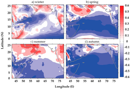
Figure 9.
The spatial correlation between zonal wind in the Arabian Sea and Multivariate ENSO Index (MEI) for the period from 1993–2018 (the sea level anomaly (SLA) data period).
During all the seasons, especially during spring and autumn, the zonal wind in the Arabian Sea displayed a negative relation with MEI, indicating that, during the positive (negative) phase of ENSO, the easterly winds in the Arabian sea are intensified (abated or lessened), thereby strengthening (weakening) the surface inflow of the Arabian Sea water into the Red Sea and regulating the surface current and sea level in the Red Sea.
A long-term analysis has also shown that sea level in the Red Sea is rising at a rate of 3.68 mm/year (p-value = 0.00), which is consistent with the global rate of the rise in sea level (3.3 mm/year) [32]. However, no significant trend is observed in the EW difference.
5. Conclusions
Based on a consecutive twenty-six-year record (1993–2018) of satellite altimetry data, this study reveals a repetitive and seasonally reversing pattern of EW difference in the sea level between the eastern and western sides of the Red Sea. The positive value of EW difference implies the sea level at the eastern side is higher than that of its western side. Climatology shows that sea level in the eastern Red Sea is clearly higher than that of the western coast from November to April, and vice versa from June to September, while the months of May and October are transition months, with a mixed pattern of sea level difference. Moreover, the summer peak of sea level in the western region is slightly higher than that of the winter peak in the eastern region by 0.3 cm. Furthermore, the seasonal mean EW difference in spring and autumn seasons have a mixed pattern, while the winter and summer clearly show and eastward and westward slope in the sea level, with a higher sea level on the eastern side during winter and on the western side during summer. Another finding coming out of this study is that the EW difference for the northern and southern regions are in phase with small differences in the range of variability; the southern Red Sea has a slightly higher range compared to that of the northern region by 0.2 cm.
The wavelet analysis result shows the presence of a significant annual cycle along with other signals of less magnitude for both the northern and southern Red Sea. After removing this annual signal, the results show the presence of two energy peaks for most of the data period, with a periodicity of <12 months and 3–7 years representing the intraseasonal and ENSO signal, respectively. The EOF result shows that EOF1 corresponds to 98% of total variability, EOF2 to 1.3% and EOF3 to 0.4%. However, this discovered EW difference in sea level has been tested for its relations with climate events, namely ENSO (MEI), IOD (DMI), and NAO. Results show that EW difference in sea level is positively related to ENSO during spring and autumn, with good positive correlation coefficients. For IOD and NAO, the relationship is weak in all the seasons.
The analysis shows that wind, buoyancy, and the polarity of eddies are the primary physical causes of this phenomenon. To illustrate this, a mean northward current in the surface layer during winter is due to the northward buoyancy flux and relatively strong SSE winds in the southern Red Sea. The NNW wind prevails in the northern Red Sea, which is in the opposite direction of the surface current, and the current continues in the northward direction, as the wind speed is relatively weak. This northward current during winter, along with the Coriolis effect, causes an eastward pile-up of water, which, alongside the dominance of anticyclonic eddies together result in a higher sea level in the eastern Red Sea compared to the western side. During summer, the NNW wind strengthens and prevails in the entire basin, which reverses the surface current direction. The southward flowing surface current results in a Coriolis-induced pile up of water towards the western side. Moreover, the dominance of eddies reverses during summer, with anticyclonic eddies dominating the western side, while cyclonic eddies dominate the eastern side. Both of these effects, the Coriolis-induced westward pile up of water and the dominance of anticyclonic eddies on the western side, together result in relatively higher sea levels in the western Red Sea during summer. The summer peak in EW difference is observed to be slightly higher than that of winter (by 0.3 cm), primarily due to the basin-wide higher surface wind speed.
Interestingly, the results have also shown that the MEI remotely influences the EW difference in the sea level of the Red Sea. A clear positive relationship is identified, especially during spring and autumn, which indicates that the easterly winds in the Arabian sea are intensified (reduced) during the positive (negative) phase of ENSO, thereby strengthening (weakening) the surface flow from the Arabian Sea into the Red Sea, leading to a larger (smaller) EW difference in sea level.
Author Contributions
Conceptualization, C.P.A.; methodology, C.P.A.; software, C.P.A.; validation, C.P.A., A.M.A.-S.; formal analysis, C.P.A.; investigation, C.P.A.; resources, C.P.A.; data curation, C.P.A.; writing—original draft preparation, C.P.A., A.M.A.-S.; writing—review and editing, C.P.A., A.M.A.-S.; visualization, C.P.A.; supervision, A.M.A.-S.; project administration, A.M.A.-S.; funding acquisition, A.M.A.-S. All authors have read and agreed to the published version of the manuscript.
Funding
This research received no external funding.
Acknowledgments
The authors thank the Archiving, Validation, and Interpretation of Satellite Oceanographic data (AVISO) and Copernicus Marine environment monitoring service for making the sea level anomaly data available to the public (http://marine.copernicus.eu/services-portfolio/access-to-products/). We also thank the National Centers for Environmental Prediction (NCEP)’s Climate Forecast System Reanalysis (CFSR, https://rda.ucar.edu/datasets/ds093.1/?hash=!access) for providing the wind data. Thanks are also extended to NOAA (National Oceanic and Atmospheric Administration) for providing the climate indices (https://www.esrl.noaa.gov/psd/). The authors are grateful to the High-Performance Computing Center at King Abdulaziz University (http://hpc.kau.edu.sa) for giving us a chance to use their facilities during the data analyses.
Conflicts of Interest
The authors declare no conflict of interest.
References
- Nidheesh, A.G.; Lengaigne, M.; Vialard, J.; Unnikrishnan, A.S.; Dayan, H. Decadal and long-term sea level variability in the tropical Indo-Pacific Ocean. Clim. Dyn. 2013, 41, 381–402. [Google Scholar] [CrossRef]
- Legeais, J.-F.; Ablain, M.; Zawadzki, L.; Zuo, H.; Johannessen, J.A.; Scharffenberg, M.G.; Fenoglio-Marc, L.; Fernandes, M.J.; Andersen, O.B.; Rudenko, S.; et al. An improved and homogeneous altimeter sea level record from the ESA Climate Change Initiative. Earth Syst. Sci. Data 2018, 10, 281–301. [Google Scholar] [CrossRef]
- Cazenave, A.; Hamlington, B.; Horwath, M.; Barletta, V.R.; Benveniste, J.; Chambers, D.; Döll, P.; Hogg, A.E.; Legeais, J.F.; Merrifield, M.; et al. Observational requirements for long-term monitoring of the global mean sea level and its components over the altimetry era. Front. Mar. Sci. 2019, 6, 14. [Google Scholar] [CrossRef]
- Grant, K.M.; Rohling, E.J.; Bronk Ramsey, C.; Cheng, H.; Edwards, R.L.; Florindo, F.; Heslop, D.; Marra, F.; Roberts, A.P.; Tamisiea, M.E.; et al. Sea-level variability over five glacial cycles. Nat. Commun. 2014, 5, 1–9. [Google Scholar] [CrossRef] [PubMed]
- Kopp, R.E.; Kemp, A.C.; Bittermann, K.; Horton, B.P.; Donnelly, J.P.; Gehrels, W.R.; Hay, C.C.; Mitrovica, J.X.; Morrow, E.D.; Rahmstorf, S. Temperature-driven global sea-level variability in the Common Era. Proc. Natl. Acad. Sci. USA 2016, 113, E1434–E1441. [Google Scholar] [CrossRef]
- Arpe, K.; Bengtsson, L.; Golitsyn, G.S.; Mokhov, I.I.; Semenov, V.A.; Sporyshev, P.V. Connection between Caspian sea level variability and ENSO. Geophys. Res. Lett. 2000, 27, 2693–2696. [Google Scholar] [CrossRef]
- Rong, Z.; Liu, Y.; Zong, H.; Cheng, Y. Interannual sea level variability in the South China Sea and its response to ENSO. Glob. Planet. Chang. 2007, 55, 257–272. [Google Scholar] [CrossRef]
- Cantin, N.E.; Cohen, A.L.; Karnauskas, K.B.; Tarrant, A.M.; McCorkle, D.C. Ocean warming slows coral growth in the central Red Sea. Science 2010, 329, 322–325. [Google Scholar] [CrossRef]
- Morcos, S.A. Physical and chemical oceanography of the Red Sea. Ocean. Mar. Biol. Annu. Rev. 1970, 8, 73–202. [Google Scholar]
- Edwards, A. Climate and oceanography. In Red Sea: Key Environments; Edwards, A.J., Head, S.M., Eds.; Pergamon Press: Oxford, UK, 1987; pp. 383–404. [Google Scholar]
- Sultan, S.A.R.; Ahmad, F.; El-Hassan, A. Seasonal variations of the sea level in the central part of the Red Sea. Estuar. Coast. Shelf Sci. 1995, 40, 1–8. [Google Scholar] [CrossRef]
- Abdelrahman, S.M. Seasonal fluctuations of mean sea level at gizan, Red Sea. J. Coast. Res. 1997, 13, 1166–1172. [Google Scholar]
- Siddall, M.; Rohling, E.; Almogi-Labin, A.; Hemleben, C.; Meischner, D.; Schmelzer, I.; Smeed, D.A. Sea-level fluctuations during the last glacial cycle. Nature 2003, 423, 853–858. [Google Scholar] [CrossRef] [PubMed]
- Siddall, M.; Smeed, D.A.; Hemleben, C.; Rohling, E.J.; Schmelzer, I.; Peltier, W.R. Understanding the Red Sea response to sea level. Earth Planet. Sci. Lett. 2004, 225, 421–434. [Google Scholar] [CrossRef]
- Hamed Ghanem, M.; Ahmad, F.; Mohammed Al-subhi, A. Heat exchange at the air-sea interface in the Red Sea by equilibrium temperature method. Indian J. Geo-Mar. Sci. 2015, 44, 1684–1689. [Google Scholar]
- Albarakati, A.M.; Ahmad, F. Variation of the surface buoyancy flux in the Red Sea. Indian J. Mar. Sci. 2013, 42, 717–721. [Google Scholar]
- Patzert, W.C. Wind-induced reversal in Red Sea circulation. Deep. Res. Oceanogr. Abstr. 1974, 21, 109–121. [Google Scholar] [CrossRef]
- Bethoux, J.P. Red Sea geochemical budgets and exchanges with the Indian Ocean. Mar. Chem. 1988, 24, 83–92. [Google Scholar] [CrossRef]
- Alawad, K.; Alsaafani, M.A.; Al-Subhi, A.M.; Alraddadi, T. Signatures of tropical climate modes on the Red Sea and gulf of aden sea level. Indian J. Geo-Mar. Sci. 2017, 46, 2088–2096. [Google Scholar]
- Taqi, A.M.; Al-Subhi, A.M.; Alsaafani, M.A.; Abdulla, C.P. Estimation of geostrophic current in the Red Sea based on sea level anomalies derived from extended satellite altimetry data. Ocean Sci. 2019, 15, 477–488. [Google Scholar] [CrossRef]
- Taqi, A.M.; Al-Subhi, A.M.; Alsaafani, M.A.; Abdulla, C.P. Improving sea level anomaly precision from satellite altimetry using parameter correction in the Red Sea. Remote Sens. 2020, 12, 764. [Google Scholar] [CrossRef]
- Woodworth, P.L.; Melet, A.; Marcos, M.; Ray, R.D.; Wöppelmann, G.; Sasaki, Y.N.; Cirano, M.; Hibbert, A.; Huthnance, J.M.; Monserrat, S.; et al. Forcing factors affecting sea level changes at the coast. Surv. Geophys. 2019, 40, 1351–1397. [Google Scholar] [CrossRef]
- Karimi, A.A.; Deng, X. Estimating sea level rise around Australia using a new approach to account for low frequency climate signals. Adv. Space Res. 2020, 65, 2324–2338. [Google Scholar] [CrossRef]
- Sofianos, S.S.; Johns, W.E. Wind induced sea level variability in the Red Sea. Geophys. Res. Lett. 2001, 28, 3175. [Google Scholar] [CrossRef]
- Manasrah, R.; Hasanean, H.M.; Al-Rousan, S. Spatial and seasonal variations of sea level in the Red Sea, 1958–2001. Ocean Sci. 2009, 44, 145–159. [Google Scholar] [CrossRef]
- Alawad, K.A.; Al-Subhi, A.M.; Alsaafani, M.A.; Alraddadi, T.M.; Ionita, M.; Lohmann, G. Large-scale mode impacts on the sea level over the Red Sea and gulf of aden. Remote Sens. 2019, 11, 2224. [Google Scholar] [CrossRef]
- Alothman, A.O.; Bos, M.; Fernandes, R.; Radwan, A.M.; Rashwan, M. Annual sea level variations in the Red Sea observed using GNSS. Geophys. J. Int. 2020, 221, 826–834. [Google Scholar] [CrossRef]
- Saji, N.H.; Goswami, B.N.; Vinayachandran, P.N.; Yamagata, T. A dipole mode in the tropical Indian Ocean. Nature 1999, 401, 360–363. [Google Scholar] [CrossRef]
- Hurrell, J.W. CLIMATE: The North Atlantic Oscillation. Science 2001, 291, 603–605. [Google Scholar] [CrossRef]
- Philander, S.G.H. El Niño Southern Oscillation phenomena. Nature 1983, 302, 295–301. [Google Scholar] [CrossRef]
- Krishna Kumar, K.; Kleeman, R.; Cane, M.A.; Rajagopalan, B. Epochal changes in Indian monsoon-ENSO precursors. Geophys. Res. Lett. 1999, 26, 75–78. [Google Scholar] [CrossRef]
- Chen, X.; Zhang, X.; Church, J.A.; Watson, C.S.; King, M.A.; Monselesan, D.; Legresy, B.; Harig, C. The increasing rate of global mean sea-level rise during 1993–2014. Nat. Clim. Chang. 2017, 7, 492–495. [Google Scholar] [CrossRef]


© 2020 by the authors. Licensee MDPI, Basel, Switzerland. This article is an open access article distributed under the terms and conditions of the Creative Commons Attribution (CC BY) license (http://creativecommons.org/licenses/by/4.0/).