Abstract
Low Earth Orbit (LEO) satellites have been widely used in scientific fields or commercial applications in recent decades. The demands of the real time scientific research or real time applications require real time precise LEO orbits. Usually, the predicted orbit is one of the solutions for real time users, so it is of great importance to investigate LEO orbit prediction for users who need real time LEO orbits. The centimeter level precision orbit is needed for high precision applications. Aiming at obtaining the predicted LEO orbit with centimeter precision, this article demonstrates the traditional method to conduct orbit prediction and put forward an idea of LEO orbit prediction by using onboard accelerometer data for real time applications. The procedure of LEO orbit prediction is proposed after comparing three different estimation strategies of retrieving initial conditions and dynamic parameters. Three strategies are estimating empirical coefficients every one cycle per revolution, which is the traditional method, estimating calibration parameters of one bias of accelerometer hourly for each direction by using accelerometer data, and estimating calibration parameters of one bias and one scale factor of the accelerometer for each direction with one arc by using accelerometer data. The results show that the predicted LEO orbit precision by using the traditional method can reach 10 cm when the predicted time is shorter than 20 min, while the predicted LEO orbit with better than 5 cm for each orbit direction can be achieved with accelerometer data even to predict one hour.
1. Introduction
More and more Low Earth Orbit (LEO) satellites have been launched to explore various phenomena on Earth [1,2], e.g., ocean altimetry [3,4], climate change, and Earth mass change [5]. In recent years, many research plans or commercial projects depending on a large number of LEO satellites have been proposed with the expectation of providing real time services on a global scale [6,7,8]. Meanwhile, the idea of a LEO enhanced Global Navigation Satellite System (LeGNSS) [9,10], where LEO satellites will transmit navigation signals to be used as navigation satellites, was put forward with such a large number of LEO satellites. With such a huge demand of real time services and different kinds of real time applications, especially for the real time Precise Point Positioning (PPP) of LeGNSS, real time centimeter level LEO orbits are the prerequisite for real time users. Near real time LEO orbits are provided for the fields of satellite occultation for meteorological purposes [11,12] and the short-latency monitoring of continental, ocean, and atmospheric mass variations [13,14]. The European Space Agency (ESA) has deployed an operational system for routine Earth Observation named Copernicus since 2014, which is designed to support a sustainable European information network by monitoring, recording, and analyzing environmental data and events around the globe [15]. The Copernicus program consists of six different families of satellites being the first three missions Sentinel -1, -2, and -3. These missions have the requirements of 8-10 cm in less than 30 min for Near Real Time (NRT) applications to 2-3 cm in less than one month for Non-Time Critical (NTC) applications [16]. The orbit accuracy of Sentinel-2A NRT products is better than 5 cm, which is better than the requirement of 10 cm as well as better than the accuracy of previous NRT LEO orbits studies [17,18]. Though the accuracy of the NRT orbit is on the centimeter level, the latency of about 30 min is not acceptable for real time positioning service of LeGNSS. Thus, predicted LEO orbit with centimeter precision should be investigated. In this study, we try to find a proper way to conduct the prediction of LEO orbits with an orbit precision on the centimeter level for real time applications, especially for the case of LeGNSS.
In order to obtain such highly accurate predicted LEO orbit for precise real time applications, precise initial conditions (position and velocity at reference time) as well as the dynamic parameters of LEO satellites used for LEO orbit prediction are required as fast as possible via LEO Precise Orbit Determination (POD). Thus, standard GNSS navigation message information is not adequate for LEO POD since the qualities of GNSS orbits and clocks are not good enough. The precision of the LEO orbit is usually at the decimeter or meter level by using the standard GNSS navigation message [12,19]. Under this circumstance, precise GNSS products should be used for LEO POD in order to get precise initial conditions and dynamic parameters of LEO satellites. Due to the Real Time Pilot Project (RTPP) launched by the International GNSS Service (IGS) in 2007 and officially operated since 2012 [20], real time precise satellite orbit and clock correction products can be obtained with Real Time Service (RTS). Currently, there are also many commercial providers, which deliver real time GPS/GNSS orbit and clock correction products, e.g., Veripos, magicGNSS, etc. Obviously, RTS can be applied to LEO POD both in the kinematic and dynamic mode. However, most onboard LEO receivers have not yet used these corrections, as it might not yet be mature enough for space applications. An alternative way is to conduct LEO POD at the analysis center with the RTS on the ground with powerful computational resources. As for the POD mode, though either kinematic or dynamic POD can achieve centimeter level orbit precision, we prefer to choose the dynamic method since the orbit of this method is consecutive and stable while that of the kinematic method is discrete. Above all, we conduct dynamic orbit determination, which estimates LEO initial conditions and dynamic parameters with real time precise GNSS orbit and clock products. Then, these dynamic parameters and initial conditions are used to do the orbit integration for times in the future, referred as orbit prediction.
Here, two issues should be taken into consideration. The first one is the update rate of the precise LEO orbit. The update rate of the LEO orbit depends on the time gap of LEO onboard observation data collection as well as the calculation time of LEO POD. The LEO onboard observations cannot be transferred to the ground stations all the time and the LEO orbit results calculated at an analysis center cannot be always uploaded to the LEO satellites unless the LEO satellites fly over the uplink and downlink stations. It is reasonable to assume that the onboard data can be collected every one hour (more than half LEO orbit revolution, personal communication with Xiangguang Meng, who is in charge of Chinese FY3C near real time POD). The second issue is the length of the orbit prediction. An empirical force model with parameters is usually utilized in dynamic LEO precise orbit determination to absorb the unmodeled part of non-gravitational forces, such as atmosphere drag and solar radiation pressure [21,22,23,24]. These parameters are important for the precision of orbit prediction if they fit the real characteristics of the unmodeled part of non-gravitational forces for the prediction arc.
Currently, some LEO satellites carry accelerometers to measure non-gravitational accelerations due to the surface forces acting on the LEO satellites, such as STAR instrument on Challenging Minisatellite Payload (CHAMP), SuperSTAR instruments on Gravity Recovery and Climate Experiment (GRACE), and GRADIO instruments on the Gravity field and steady-state Ocean Circulation Explorer (GOCE). These instruments have extreme sensitivity and unprecedented accuracy with up to , , and for STAR, SuperSTAR, and GRADIO, respectively. The measurement from the accelerometers has to be calibrated when processing the measurement from their missions to produce the gravity field models [25]. Researchers proposed a calibration method, which displays approximately constant scales and slowly changing biases for both GRACE A and B satellites [26]. Numerous acceleration spikes related to the switching activity in the circuits of onboard heaters are identified and analyzed [27]. It is a possibility to use the accelerometer data for LEO POD instead of empirical force models [28], [29]. The calibration parameters of the accelerometer such as scale and bias should be estimated together with the LEO initial position and velocity when using accelerometer data. Inspired by the stability of the calibration parameters of the accelerometer, we try to use accelerometer data to predict the LEO orbit instead of empirical force models. We compare two methods of accelerometer data calibrations with respect to the empirical force models in order to develop the potential LEO orbit prediction process strategy.
The article is structured as follows. Different possible procedures of LEO orbit prediction are discussed in the next section. The corresponding methods of LEO orbit prediction are conducted as well as the analysis of calibration parameters of accelerometers in the following sections. Then the extensive LEO orbit prediction experiments are carried out, including the impact of different integration intervals on the LEO orbit precision. Research findings and concluding remarks are given in the following section. Finally, practical issues about widespread use of an accelerometer are discussed.
2. LEO Orbit Prediction Procedure
The procedures of LEO orbit prediction for real time applications will be clarified. The simplified demonstration and flowchart are shown as Figure 1.

Figure 1.
Procedures of Low Earth Orbit (LEO) orbit prediction. The LEO onboard Global Navigation Satellite System (GNSS) and accelerometer data are downlinked and transferred to the analysis center and processed there. The estimated initial condition states of LEO as well as the dynamic parameters are then uplinked to LEO satellites and the predicted LEO orbit is integrated onboard.
The downlink stations receive the LEO onboard GNSS observations and accelerometer data when LEO satellites pass over the downlink stations. LEO POD can be conducted in the analysis center with real time GNSS products from RTS. LEO initial conditions and the corresponding dynamic parameters can be obtained after LEO POD. Then these parameters could be uplinked to the corresponding LEO satellites for orbit prediction and real time LEO orbits can be broadcast to the users for real time applications. As is well known, the length of LEO orbit prediction determines the precision of real time LEO orbits. However, the length of orbit prediction is fully dependent on the time gap of LEO onboard observation data collection and computation time of LEO POD. It takes about 1.5–1.7 h for one LEO satellite cycle with the altitude from 500 to 1000 km. For the computation time of LEO POD with a 24 h arc length, it takes about 10 min for one LEO satellite at the GFZ server. In general, LEO satellites fly overhead a ground station for 10–15 min. It is possible to download the observation data, calculate LEO orbit and inject the data to the corresponding LEO satellites in 15 min. Then after a half cycle of about 50 min, this procedure can be done again at another downlink and uplink station. Under this circumstance, one hour is enough for LEO orbit prediction and we took this length for our following analysis. For the sake of insurance, we also prepared two hours as backup if the orbital elements could not be uplinked in time and were delayed to be uplinked at the next uplink station. The timeline of data process is shown in Figure 2. If the time gap of LEO onboard observation data collection is shorter, the length of orbit prediction time can be even shorter.
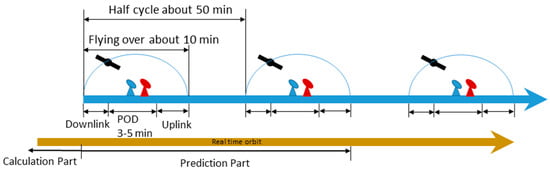
Figure 2.
Timeline of the data process.
With these procedures, we proposed three strategies to fulfill LEO prediction. We took GRACE-A data for example with its data from Day Of Year (DOY) 010, 2007 to DOY 360, 2007. As aforementioned, the LEO initial conditions and dynamic parameters determinate the precision of predicted LEO orbits. The accelerometer measures all non-gravitational forces acting on the satellite. However, the measurement has to be calibrated in terms of bias and scale when they are used to process orbit determination. The bias and scale have to be estimated together with the LEO initial position and velocity. The calibration model can be written as
where denotes the non-gravitational acceleration. denotes the bias vector. denotes the scale matrix. denotes the non-gravitational measurement. Note both and are in the GRACE Science Reference Frame (SRF), while LEO POD is conducted in the inertial system. Thus, one needs to transform from SRF to the inertial frame, which is
where is the transform matrix from SRF to the inertial frame.
The proposed three strategies are mainly focused on the determination of dynamic parameters in LEO POD and they are as follows.
Strategy 1: Accelerometer data are used with the calibration parameters of biases and scale factors in each axis for one arc, which are named as BX, BY, BZ, KX, KY, and KZ. For simplicity and easy reading, ACC_B_K is used in the following study referring to this strategy.
Strategy 2: Accelerometer data are used with the calibration parameters of biases in each axis every 60 min, which are named as BX, BY, and BZ and scale factors for three directions are equal to one. This strategy is called ACC_B in the following.
Strategy 3: Empirical force models are used with the dynamic coefficients of Ca, Sa, Cc, and Sc for along- and cross-track directions (cosine/sine), and a scale factor for the atmospheric drag every one cycle per revolution. EMP is used referring to this strategy in the following.
Strategy 1 (ACC_B_K) and 2 (ACC_B) are different at the estimation of calibration parameters of the accelerometer, which are based on the GFZ GRACE Level-2 processing standards document [30,31]. Strategy 3 (EMP) was conducted to show the precision of predicted LEO orbits with empirical force models. Actually, there is a shortcoming with the method using accelerometer data, for which orbit prediction must be conducted onboard, since real time accelerometer data should be acquired. The empirical method is simple that one can conduct the orbit prediction at the analysis center, then uplink the LEO orbits to the corresponding LEO satellites.
The batch least square approach was used to estimate the LEO initial position and velocity as well as dynamic parameters. The force models, observation models, and the parameters to be estimated in LEO POD are listed in Table 1.

Table 1.
Force models, observation models, and estimated parameters of LEO POD with different strategies.
As recorded by the GRACE Science data system monthly report, the Disabling of Supplemental Heater Lines (DSHL) of GRACE-A would cause temperature control on accelerometer to be stopped. The cool down of the accelerometer caused the accelerometer biases to change and the reheating of the accelerometer returned the accelerometer biases to near nominal values after some days, which would affect POD by using accelerometer data. For this reason, these days are excluded in the following analysis, such as the data from 17th to 21st January (DOY: 017 to 021, 2007) and from 22nd to 26th November (DOY: 326 to 330, 2007). We used the slide window process to simulate the real time process. The length of slide window is equal to the length of prediction time. So, we have 24 sets of results in one day if the length of prediction time is one hour.
3. Analysis of Dynamic Parameters
In this section, we first checked the precision of LEO orbits by using precise GNSS products with those three strategies. Here, we used CODE (Center for Orbit Determination in Europe) precise GPS orbit and 30 s clock products since there was no real time precise orbit and clock products in 2007 (ftp://cddis.gsfc.nasa.gov/pub/gps/products, [41]). Furthermore, one has to collect and store real time orbit and clock corrections by themselves since no public archive is available for the storage of previous real time orbit and clock products. More details about the impact on LEO POD with real time products and final products can be found in the Appendix. The Precise Science Orbits (PSO) of GRACE-A provided by Jet Propulsion Laboratory (JPL) was used as references for our orbit evaluation in this article (https://podaac-tools.jpl.nasa.gov/drive/files/allData/grace/L1B/JPL). Then the accelerometer calibration parameters as well as the parameters of empirical models were also investigated for the first two strategies. Figure 3 shows the averaged Root Mean Square (RMS) values for along-track, cross-track, and radial directions with the three strategies, respectively. The corresponding averaged RMS values of all days for three directions are shown in Table 2.
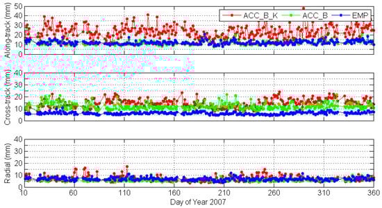
Figure 3.
Averaged Root Mean Square (RMS) values for along-track, cross-track, and radial directions with the three strategies.
Table 2.
Averaged RMS values on all days for three directions with three strategies.
In general, the RMS values are smallest for all directions when empirical force models are used. These empirical models can efficiently absorb the unmodeled part of the non-gravitational forces. The averaged RMS values for all days were 12.1 mm, 6.2 mm, and 6.8 mm for along-track, cross-track, and radial direction, respectively. For radial direction, the RMS values of the two strategies using accelerometer data were nearly the same as using the empirical force models with about 6.8 mm, while the RMS values of cross-track direction were larger than that of empirical method, which were 14.3 mm and 11.9 mm for the ACC_B_K method and ACC_B method. This is mainly caused by the sensitivity of the accelerometer [42]. The more sensitive axes point in the flight and radial directions, the less sensitive axis points in the cross-track direction [26]. The precision of the sensitive axes is specified to be 10−10 m/s2 and that of the less sensitive axis 10−9 m/s2 [27]. The RMS values of the along-track direction for the strategy of estimating the accelerometer bias every one hour and empirical forces were almost the same at about 12.0 mm while the strategy of estimating the accelerometer bias and scale for one day were worse than those two strategies with 23.3 mm. Such a difference may be caused by the number of estimated parameters. The number of estimated dynamic parameters of the three strategies is 6 (BX, BY, BZ, KX, KY, and KZ), 72 (BX, BY, and BZ every one hour for 24 h, 24 × 3 = 72), and 80 (Ca, Sa, Cc, Sc, and a scale factor every one cycle per revolution for 24 h, 24/1.5 × 5 = 80), respectively. In the least square estimator, the more parameters, the smaller the fitted residuals if all parameters are estimable.
The initial conditions and dynamic parameters estimated from the POD process are then used for the LEO orbit prediction. It is of great importance to analyze dynamic parameters since they will have a direct effect on the orbit precision for orbit prediction. If only one set dynamic parameters is estimated for one arc, then these estimated parameters are used for LEO orbit prediction, such as strategy 1 (ACC_B_K). If there are more than one set of dynamic parameters estimated like strategy 2 (ACC_B) and 3 (EMP), one has to firstly investigate the characteristics of the dynamic parameters and then decide the way to predict the LEO orbit. Figure 4 shows the accelerometer bias parameters for strategy 2.
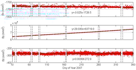
Figure 4.
Accelerometer bias parameters for strategy 2. The data between black dashed lines are excluded because of the change of the controller onboard or abnormal behavior of accelerometer. Black lines are the linear fitting line. The corresponding fitting results are also shown in each panel.
The behavior of three biases was different for the three directions. By linear fitting, we could find that biases in the y direction show a clear smooth trend in the year. It changed about 10,450 nm/s2 in the year. For the x direction, there was also a small trend, which was about -9 nm/s2 in 2007. Biases in the z direction keep quite stable, which was only 1.3 nm/s2 in the year. Due to this increased or decreased trend of the biases, it may not be appropriate using the last set of accelerometer calibration parameters to conduct the real time orbit prediction and linear fitting and an extrapolation should be used when doing the orbit integration for real time LEO orbits. Figure 5 shows the averaged RMS of calibration parameters’ differences between using the extrapolated calibration parameters for one hour and the estimated ones as well as the averaged RMS of calibration parameters’ differences between using the last set of calibration parameters and estimated ones for each arc.
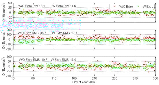
Figure 5.
Averaged RMS of calibration parameters’ differences between using the extrapolated calibration parameters and the estimated ones as well as the averaged RMS of calibration parameters’ differences between using the last set of calibration parameters and the estimated ones for each arc. “W/O Extro” means without extrapolated and “W Extro” means with extrapolation.
From Figure 5, we can see that the extrapolated calibration parameters are much closer to the estimated ones, which means the precision of the predicted orbit by using extrapolated calibration parameters should be higher than that of using the last set of calibration parameters. The accelerometer bias in the y direction shows the largest difference since this direction is the least sensitive for the accelerometer instrument, which is pointing to the cross-track direction of the LEO orbit while the bias in the x direction shows the smallest difference. In the following LEO orbit prediction analysis, we will use the extrapolation calibration parameters for orbit prediction with strategy 2.
Figure 6 shows the dynamic parameters in the EMP method. It shows that the dynamic parameters are not stable, especially for the Sa and Ca terms, which are used for compensating the unmodeled part of the along-track component. They are quite different from day to day. This also implies that the non-gravitational force models used in the POD are not accurate enough and the dynamic parameters have to be estimated in order to absorb the unmodeled part of non-gravitation. It is not appropriate to use the extrapolate method to obtain dynamic parameters for orbit prediction like the ACC_B method since these parameters fluctuated and are hard to predict. So, the last set of dynamic parameters was adopted to predict the orbit in the following parts for the EMP method.
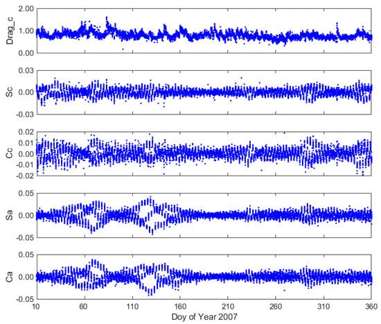
Figure 6.
Dynamic parameters estimated from Strategy 3.
4. Results of LEO Orbit Prediction
After conducting LEO POD, the initial conditions as well as the dynamic parameters can be uplinked to the corresponding LEO satellites. Then the processor on LEO satellites can do orbit prediction/propagation for real time applications. We used one hour for orbit prediction as mentioned before. One issue should be clarified here. If we used the EMP method in which empirical force models are applied, the orbit prediction could also be conducted at the analysis center in advance since no real time onboard observations are required whereas for the ACC_B_K and ACC_B method, it must be conducted onboard because real time accelerometer data must be used.
The initial conditions and the dynamic parameters have great impact on the precision of LEO orbit. For the EMP method, the last set of empirical coefficients were chosen for real time orbit integration as usual and for the ACC_B_K method there was only one set of calibrations parameters for each direction including scales and biases for the orbit integration. For the ACC_B method, we used a linear fitting for the previous 24-h arc since an obvious trend could be found in these biases, and then extrapolated the biases according to the integration time.
The differences between PSO and predicted orbits were calculated for the orbit evaluation and their User Ranging Error (URE) were also calculated and compared. URE provides the average range error in the line-of-sight direction at a global scale. Its computation is related to the maximum satellite coverage on the Earth’s surface. The coverage depends on the angular range of the satellite, which is the angle of the emission cone with respect to the boresight direction. With the angular range of LEO satellites at the altitude of 500 km being about 68.02°, the URE can be approximately determined as [8,9,43]:
Figure 7 shows the averaged RMS values of a one hour predicted orbit in three directions with the three strategies. The corresponding averaged RMS values of all days for each direction with different strategies are shown at the top left of each panel.
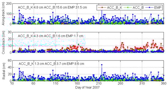
Figure 7.
Averaged RMS values for the three directions with three strategies for an orbit prediction of one hour.
It is easy to find out that the ACC_B_K strategy shows the best results, especially for along-track direction at 4.8 cm while the ACC_B and EMP strategies were at 15.6 cm and 31.5 cm. For the radial direction, the RMS values were 1.7 cm, 3.7 cm, and 8.6 cm for the ACC_B_K, ACC_B, and EMP strategy, respectively. The RMS value of cross-track direction for the ACC_B_K strategy was 4.3 cm, which was worse than the other two strategies with 1.6 cm and 1.7 cm. As Figure 8 shows, the averaged URE values for the three strategies were 4.4 cm, 10.1 cm, and 20.3 cm, respectively.
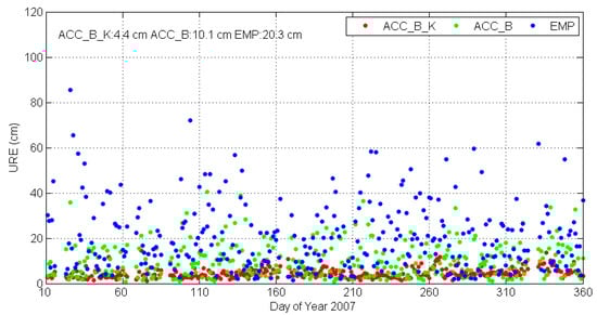
Figure 8.
User Ranging Error (URE) of a real time LEO orbit for three different strategies.
It is easy to understand that predicted LEO orbit precision by using accelerometer data were better than that of using empirical force models since accelerometer data could better reflect the non-gravitational forces than that of the empirical force models. We found that with the method of strategy 1 (ACC_B_K), the predicted LEO orbit precision shows a better result in the along and radial directions than with strategy 2 (ACC_B), though the calculation part (orbit determination part) of ACC_B_K of the along-track and radial directions was worse than those of ACC_B. We calculated the differences of the predicted non-gravitational acceleration between ACC_B_K and the corresponding non-gravitational acceleration calculated from estimated biases and the scale factor as well as the differences of predicted non-gravitational acceleration between ACC_B and the corresponding non-gravitational acceleration calculated from estimated biases for a one hour prediction, as shown in Figure 9.
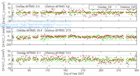
Figure 9.
Differences of predicted non-gravitational acceleration between the ACC_B_K method and the calculated ones as well as the differences of predicted non-gravitational acceleration between the ACC_B method and the calculated ones for a one hour prediction in each direction. “Oneday dif” means the ACC_B_K method and “Onehour dif” means the ACC_B method.
From Figure 9, we can see that the difference of non-gravitational accelerations in the x direction (orbit along-track direction) and z direction (radial direction) with the ACC_B_K method were much smaller than those of the ACC_B method, which means that the along-track and radial direction precision of the prediction part with ACC_B_K should be better than those of the ACC_B method. For the cross-track direction (y direction of acceleration), the differences between the predicted acceleration and the calculated one with the ACC_B_K method were larger than that of the ACC_B method, which corroborated the worse results of the cross-track direction with the ACC_B_K method.
In conclusion, one set of scales and biases for each direction reflected the calibration parameters of the accelerometer for the long term while one set of biases every hour reflected for the short term. For orbit prediction for less than 20 min, the precision of all orbit components with all strategies was better than 10 cm. This means that if the interval of the uplink and downlink was shorter than 20 min, all strategies could be used for real time LEO POD. For orbit prediction for more than 20 min, the best way to realize the real time LEO precise orbit determination is by using accelerometer data with the estimation of one set of scales and biases for each direction. In this way, less than a 5 centimeter level of LEO orbit precision can be achieved for the one hour LEO orbit prediction, which satisfies the demand of a centimeter level requirement mentioned in the Introduction section.
Usually, most precise positioning users care more about the orbit errors for every epoch while not for the averaged ones over one hour. Figure 10 shows RMS values of LEO orbits for three directions of every 10 min over a one hour prediction time period. The great increase of along-track RMS values with the empirical method can be easily found, which is from about 5.0 cm at 10 min to approximately 49.4 cm over one hour. However, the method with accelerometer data with one set of biases and scales for each direction shows a stable RMS of 4.9 cm, 4.0 cm, and 1.2 cm in the along-track, cross-track, and radial directions all the time, respectively.
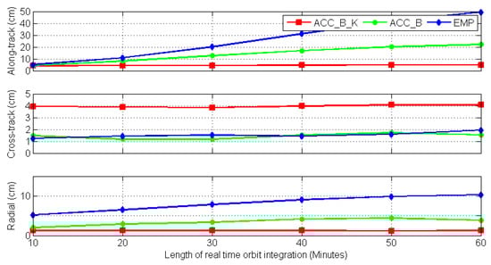
Figure 10.
RMS values of LEO orbits for the along-track, cross-track, and radial direction for every 10 min over a one hour period.
The corresponding URE for every 10 min is shown in Figure 11. The method with accelerometer data with one set of biases and scales for each direction shows the most stable results about 4.6 cm even if the integration time is one hour while the method of empirical and accelerometer data with one-hour biases for each direction shows an increased trend, from about 4.6 cm at 0-10 min to 31.4 cm and 14.0 cm within 50-60 min.
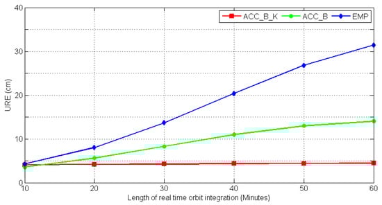
Figure 11.
URE for every 10 min over a one hour orbit prediction.
As mentioned above in the “LEO orbit prediction procedure”, if the orbital elements do not uplink in time, one has to wait until the next uplink, which means a delay of nearly two hours. The RMS values of LEO orbits for three directions with another one hour prediction and the corresponding URE values are shown in Figure 12.
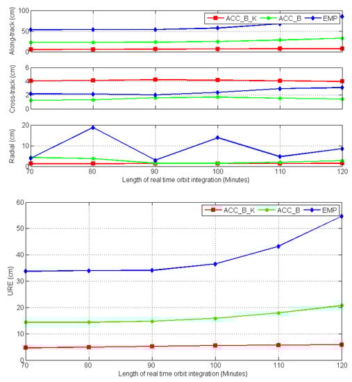
Figure 12.
RMS values of LEO orbits for the along-track, cross-track, and radial direction for another one hour and corresponding URE values.
We could easily find that the method with accelerometer data with one set of biases and scales for each direction (ACC_B_K) still shows the most stable results while the method with empirical models (EMP) fluctuated, especially in the radial component. The RMS value for the along-track component could be at one meter for the method with empirical models while it is still better than 10 cm for the method with one set of biases and scales.
5. Conclusions
With the development of the LEO related missions and applications, there will be a great demand of real time LEO precise orbit. In this study, three strategies with estimation of different dynamic parameters were conducted and the conclusions are summarized as follows
- (1)
- The precision of LEO satellites orbits could reach the centimeter level with estimation of different kinds of dynamic parameters if precise GNSS products were adopted. However, under the current circumstances, RTS was not available for onboard processing. For the demand of the real time precise LEO orbit, at least a one-hour orbit prediction should be adopted.
- (2)
- For the current GNSS technology, LEO orbit prediction by using accelerometer data was feasible. Precision of one hour predicted LEO satellite orbits with initial conditions and dynamic parameters estimated with a 24 h arc could reach the centimeter level by using accelerometer data while that using empirical force models was at the decimeter level.
- (3)
- For the LEO orbit prediction over 20 min, the predicted LEO orbit precision with estimation of one set of biases and scales for each direction (strategy 1) was better than that of biases for each direction every 60 min (strategy 2), though the calculated orbit precision with the latter was better than the former method.
- (4)
- If there were enough uplink and downlink stations, which mean the interval of uplink and downlink could be shorter than 20 min, all these three strategies could be adopted for the real time applications.
On all accounts, the accelerometer data had great potential to do the LEO orbit prediction for real time applications in the near future.
6. Discussions
This article aimed at investigating centimeter level precision of LEO orbit prediction for real time applications. It is a good replacement of using accelerometer data instead of empirical force models when conducting LEO orbit prediction. Three strategies with estimation of different dynamic parameters were conducted. The results show that with our proposed method, the LEO orbit precision could reach the centimeter level and even predicting within two hours. Two more practical issues should be clarified.
The first one is the feasibility of widespread use of accelerometers. The idea of using accelerometers for orbit prediction is a good idea and it was already shown in this study. However, the accelerometers we used were of high quality for specific missions, such as a gravity mission. Such accelerometers may be too expensive for the mass market. Concerning this issue, experiments (one can add colored or white noise in the accelerometer data) could be conducted in the future to check the tolerance of accelerometer data with respect to the precision of orbit prediction.
The second issue is the time gap of LEO onboard observation data collection. We took GRACE-A as example, which has an inclination of 89°. It is quite easy to have a continuous coverage for sustained period (half cycle of the LEO orbital period) where the uplink and downlink station are located at high latitudes (north and south). However, more uplink and downlink stations are needed of LEO satellites with low orbital inclination to meet the max length of the LEO orbit prediction (such as about 20 min for GRACE-A to keep the centimeter precision of the orbit prediction with empirical models). The distribution of the uplink and downlink stations for different inclinations of LEO satellites should be investigated to guarantee the time gap of onboard data collection.
Author Contributions
All authors contributed to the writing of this manuscript. H.G., B.L., and M.G. conceived the idea of employing accelerometer data to conduct LEO orbit prediction. H.G. and L.N. processed the data and investigated the results. M.G., B.L., and H.S. validated the data. All authors have read and agreed to the published version of the manuscript.
Funding
This study is sponsored by National Natural Science Foundation of China (41874030), The Scientific and Technological Innovation Plan from Shanghai Science and Technology Committee (18511101801), and The National Key Research and Development Program of China (2017YFA0603102), and the Fundamental Research Funds for the Central Universities.
Acknowledgments
Thanks to Physical Oceanography Distributed Active Archive Center (PO. DAAC) of JPL for providing the raw GNSS observations and post-processed reduced dynamic orbit of GRACE-A and GRACE-C. The GNSS observations and orbit products are available from https://podaac-tools.jpl.nasa.gov/drive/files/allData/grace/L1B/JPL and https://podaac-tools.jpl.nasa.gov/drive/files/allData/gracefo/L1B/JPL/RL04/ASCII for GRACE-A and GRACE-C, respectively. We are also grateful to CODE and GFZ real time group for providing precise GPS final products and real time products, respectively.
Conflicts of Interest
The authors declare no conflict of interest.
Abbreviations and Acronyms
The following acronyms and abbreviations are used in this manuscript:
| CHAMP | Challenging Minisatellite Payload |
| CODE | Center for Orbit Determination in Europe |
| DOY | Day of Year |
| DSHL | Disabling of Supplemental Heater Lines |
| ESA | European Space Agency |
| GFZ | GeoForschungsZentrum |
| GNSS | Global Navigation Satellite System |
| GOCE | Gravity field and steady-state Ocean Circulation Explorer |
| GPS | Global Positioning System |
| GRACE | Gravity Recovery and Climate Experiment |
| GRACE-FO | Gravity Recovery and Climate Experiment Follow-On |
| IGS | International GNSS Service |
| JPL | Jet Propulsion Laboratory |
| LEO | Low Earth Orbit |
| LeGNSS | Leo enhanced Global Navigation Satellite System |
| NRT | Near Real Time |
| NTC | Non Time Critical |
| POD | Precise Orbit Determination |
| PPP | Precise Point Positioning |
| RMS | Root Mean Square |
| RTPP | Real Time Pilot Project |
| RTS | Real Time Service |
| SRF | Science Reference Frame |
| ACC_B_K | Strategy of estimating bias and scale of accelerometer |
| ACC_B | Strategy of estimating bias of accelerometer |
| EMP | Strategy of estimation empirical dynamic parameters |
Appendix
The LEO data used in the article is GRACE-A data in 2007 when no real time precise orbit and clock products are available. Until now, there is no public archive available for the storage of real time orbit and clock products. Thanks to the GFZ real time working group, they have stored these real time products since April 26th, 2018, which make it possible for us to demonstrate the orbit difference of LEO POD by using precise GPS products and real time products. We updated our software recently to conduct GRACE Follow On (GRACE-FO) POD since GRACE mission was ended in October, 2017. GRACE-FO mission is the successor of the GRACE mission, the orbit of GRACE-FO satellite (GRACE-C and GRACE-D) is nearly the same as that of GRACE with the orbital inclination of 89 degree. Moreover, GRACE-FO observatory builds on the design of the original GRACE, but incorporates a number of improvements based on lessons learned [44].
In this part, we firstly evaluate one week GFZ real time products (2019, DOY 216-222) with respect to CODE final products. Then GRACE-C POD with empirical force model is conducted to demonstrate how much difference is expected due to the use of real time products instead of precise CODE products.

Figure A1.
RMS of GPS orbit difference (top) and STD of GPS clock difference (bottom) between CODE products and GFZ real time products.
Figure A1 shows the RMS values of GPS orbit difference and STD of GPS clock difference between CODE products and GFZ real time products. The averaged RMS values of all GPS satellites for along-track, cross-track, and radial directions are 3.5 cm, 2.7 cm, and 2.4 cm, respectively. The STD values of GPS clock difference are generally smaller than 0.2 ns for all GPS satellites. The averaged STD value of all satellites is 0.14 ns, which is about 4.0 cm in distance. With these products, GRACE-C satellite POD is conducted. Since GRACE-FO is built on the design of GRACE, all the force models used for GRACE can be adopted for GRACE-FO as shown in Table 1. The PSO of GRACE-C provided by JPL are used as references for our orbit evaluation (https://podaac-tools.jpl.nasa.gov/drive/files/allData/gracefo/L1B/JPL/RL04/ASCII). The averaged RMS of GRACE-C orbits with respect to the PSO is shown in Figure A2.

Figure A2.
RMS of GRACE-C orbit with respect to JPL PSO orbits by using CODE final products and GFZ real time products.
From Figure A2, we can see that the RMS values of orbit by using GFZ real time products are slightly larger than those of CODE final products. The differences are about 8 mm, 3 mm, and 2 mm for along-track, cross-track, and radial directions, respectively. By using real time products, the orbit precision for 3D will degrade about 1 cm.
References
- Li, D. China’s first civilian three-line-array stereo mapping satellite: ZY3. Acta Geod. Cartogr. Sin. 2012, 41, 317–322. [Google Scholar]
- Li, D.; Shen, X. On civil-military integrated space-based real-time information service system. Geomat. Inf. Sci. Wuhan Univ. 2017, 42, 1501–1505. [Google Scholar]
- Fu, L.L.; Christensen, E.J.; Yamarone, C.A.; Lefebvre, M.; Menard, Y.; Dorrer, M.; Escudier, P. TOPEX/POSEIDON mission overview. J. Geophys. Res. Ocean. 1994, 99, 24369–24381. [Google Scholar] [CrossRef]
- Zhang, Q.; Zhang, J.; Zhang, H.; Wang, R.; Jia, H. The study of HY2A satellite engineering development and in-orbit movement. Eng. Sci. 2013, 80, 12–18. [Google Scholar] [CrossRef]
- Tapley, B.D.; Bettadpur, S.; Watkins, M.; Reigber, C. The gravity recovery and climate experiment: Mission overview and early results. Geophys. Res. Lett. 2004, 31, 09607. [Google Scholar] [CrossRef]
- Maine, K.; Devieux, C.; Swan, P. Overview of IRIDIUM satellite network. In Proceedings of the WESCON, San Francisco, CA, USA, 13–16 November 1995; pp. 483–490. [Google Scholar]
- Hanson, W.A. In Their Own Words: OneWeb’s Internet Constellation as Described in Their FCC Form 312 Application. New Space 2016, 4, 153–167. [Google Scholar] [CrossRef]
- Li, B.; Ge, H.; Ge, M.; Nie, L.; Shen, Y.; Schuh, H. LEO enhanced Global Navigation Satellite System (LeGNSS) for real-time precise positioning services. Adv. Space Res. 2019, 63, 73–93. [Google Scholar] [CrossRef]
- Reid, T.G.; Neish, A.M.; Walter, T.F.; Enge, K.P. Leveraging Commercial Broadband LEO Constellations for Navigation. In Proceedings of the ION GNSS+ 2016, Portland, OR, USA, 12–16 September 2016; pp. 2300–2314. [Google Scholar]
- Ge, H.; Li, B.; Ge, M.; Zang, N.; Nie, L.; Shen, Y.; Schuh, H. Initial Assessment of Precise Point Positioning with LEO Enhanced Global Navigation Satellite Systems (LeGNSS). Remote Sens. 2018, 10, 984. [Google Scholar] [CrossRef]
- Montenbruck, O.; Gill, E.; Kroes, R. Rapid orbit determination of LEO satellites using IGS clock and ephemeris products. GPS Solut. 2005, 9, 226–235. [Google Scholar] [CrossRef]
- Montenbruck, O.; Ramos-Bosch, P. Precision real-time navigation of LEO satellites using global positioning system measurements. GPS Solut. 2008, 12, 187–198. [Google Scholar] [CrossRef]
- Gruber, C.; Gouweleeuw, B. Short-latency monitoring of continental, ocean- and atmospheric mass variations using GRACE intersatellite accelerations. Geophys. J. Int. 2019, 217, 714–728. [Google Scholar] [CrossRef]
- Purkhauser, A.F.; Pail, R. Next generation gravity missions: Near-real time gravity field retrieval strategy. Geophys. J. Int. 2019, 217, 1314–1333. [Google Scholar] [CrossRef]
- Fernandez, J.; Escobar, D.; Agueda, A.; Femenias, P. Sentinels POD service operations. In Proceedings of the SpaceOps 2014 Conference, Pasadena, CA, USA, 5–9 May 2014; p. 1929. [Google Scholar]
- Fernandez, J.; Ayuga, F.; Fernandez, C.; Peter, H.; Femenias, P. Copernicus POD service operations. In Proceedings of the SpaceOps 2016 Conference, Daejeon, Korea, 16–20 May 2016; p. 2385. [Google Scholar]
- Rodríguez-Portugal, F.S.; Fadrique, F.M.; Maté, A.A.; Damiano, A. Near real-time precise orbit determination for LEO satellites. In Proceedings of the 18th International Symposium on Space Flight Dynamics (ESA SP-548), Munich, Germany, 11–15 October 2004; p. 175. [Google Scholar]
- Arbinger, C.; D’Amico, S. Impact of orbit prediction accuracy on low earth remote sensing flight dynamics operations. In Proceedings of the 18th International Symposium on Space Flight Dynamics, Munich, Germany, 11–15 October 2004; pp. 73–78. [Google Scholar]
- Wang, F.; Gong, X.; Sang, J.; Zhang, X. A Novel Method for Precise Onboard Real-Time Orbit Determination with a Standalone GPS Receiver. Sensors 2015, 15, 30403–30418. [Google Scholar] [CrossRef] [PubMed]
- Caissy, M.; Agrotis, L.; Weber, G.; Hernandez-Pajares, M.; Hugentobler, U. The International GNSS real-time service. GPS World 2012, 22, 52–58. [Google Scholar]
- Schutz, B.E.; Tapley, B.D.; Abusali, P.A.M.; Rim, H.J. Dynamic orbit determination using GPS measurements from TOPEX_POSEIDON. Geophys. Res. Lett. 1994, 21, 2179–2182. [Google Scholar] [CrossRef]
- Jäggi, A.; Hugentobler, U.; Beutler, G. Pseudo-Stochastic Orbit Modeling Techniques for Low-Earth Orbiters. J. Geod. 2006, 80, 47–60. [Google Scholar] [CrossRef]
- Kang, Z.; Tapley, B.D.; Bettadpur, S.; Ries, J.; Nagel, P.; Pastor, R. Precise orbit determination for the GRACE mission using only GPS data. J. Geod. 2006, 80, 322–331. [Google Scholar] [CrossRef]
- Van Den Ijssel, J.; Encarnação, J.; Doornbos, E.; Visser, P. Precise science orbits for the Swarm satellite constellation. Adv. Space Res. 2015, 56, 1042–1055. [Google Scholar] [CrossRef]
- Kang, Z.; Bettadpur, S.; Tapley, B.D.; Cheng, M.; Ries, J. Determination of CHAMP Accelerometer Calibration Parameters. In First CHAMP Mission Results for Gravity, Magnetic and Atmospheric Studies, 1st ed.; Reigber, C., Lühr, H., Schwintzer, P., Eds.; Springer: Berlin, Germany, 2003; pp. 19–25. [Google Scholar]
- Bezděk, A. Calibration of accelerometers aboard GRACE satellites by comparison with POD-based nongravitational accelerations. J. Geodyn. 2010, 50, 410–423. [Google Scholar] [CrossRef]
- Flury, J.; Bettadpur, S.; Tapley, B.D. Precise accelerometry onboard the GRACE gravity field satellite mission. Adv. Space Res. 2008, 42, 1414–1423. [Google Scholar] [CrossRef]
- Kang, Z.; Tapley, B.D.; Bettadpur, S.; Ries, J.; Nagel, P. Precise orbit determination for GRACE using accelerometer data. Adv. Space Res. 2006, 38, 2131–2136. [Google Scholar] [CrossRef]
- Van Helleputte, T.; Visser, P. GPS based orbit determination using accelerometer data. Aerosp. Sci. Technol. 2008, 12, 478–484. [Google Scholar] [CrossRef]
- Flechtner, F. GFZ Level-2 Processing Standards Document for Level-2 Product Release 0004, GRACE 327-743 (GR-GFZ-STD-001); GFZ, Oberpfaffenhofen: Wessling, Germany, 2007. [Google Scholar]
- Dahle, C.; Flechtner, F.; Gruber, C.; Koenig, D.; Koenig, R.; Michalak, G.; Neumayer, K.H. GFZ GRACE Level-2 Processing Standards Document for Level-2 Product Release 0005, Scientific Technical Report STR12/02-Data. ISSN 1610-0956; GFZ, Oberpfaffenhofen: Wessling, Germany, 2013. [Google Scholar]
- Förste, C.; Bruinsma, S.; Shako, R.; Marty, J.; Flechtner, F.; Abrikosov, O.; Dahle, C.; Lemoine, J.; Neumayer, K.; Biancale, R.; et al. A new release of EIGEN-6: The latest combined global gravity field model including LAGEOS, GRACE and GOCE data from the collaboration of GFZ Potsdam and GRGS Toulouse. In Proceedings of the EGU General Assembly Conference Abstracts, Vienna, Austria, 22–27 April 2012; p. 2821. [Google Scholar]
- Standish, E.M. JPL Planetary and Lunar Ephemerides, DE405/LE405; JPL IOM 312.F-98-048; Jet Propulsion Laboratory: Pasadena, CA, USA, 1998. [Google Scholar]
- Petit, G.; Luzum, B. IERS Conventions 2010, IERS Technical Note No.36; Verlag des Bundesamts für Kartographie und Geodäsie: Frankfurt am Main, Germany, 2010. [Google Scholar]
- Savcenko, R.; Bosch, W. EOT11a—Empirical Ocean Tide Model from Multi-Mission Satellite Altimetry, Report No. 89; Deutsches Geodätisches Forschungsinstitut: Munich, Germany, 2012. [Google Scholar]
- Berger, C.; Biancale, R.M., III; Barlier, F. Improvement of the empirical thermospheric model DTM: DTM94–a comparative review of various temporal variations and prospects in space geodesy applications. J. Geod. 1998, 72, 161–178. [Google Scholar] [CrossRef]
- Bettadpur, S. GRACE Product Specification Document. CSR-GR-03-02, v4.6; Center for Space Research, University of Texas at Austin: Austin, TX, USA, 2012. [Google Scholar]
- Wu, J.T.; Wu, S.C.; Haij, G.A.; Bertiger, W.I.; Lichten, S.M. Effects of antenna orientation on GPS carrier phase. Manusc. Geod. 1993, 18, 91–98. [Google Scholar]
- Case, K.; Kruizinga, G.; Wu, S.C. GRACE Level 1B Data Product User Handbook; JPL D-22027; California Institute of Technology: Pasadena, CA, USA, 2010. [Google Scholar]
- Schmid, R.; Steigenberger, P.; Gendt, G.; Ge, M.; Rothacher, M. Generation of a consistent absolute phase-center correction model for GPS receiver and satellite antennas. J. Geod. 2007, 81, 781–798. [Google Scholar] [CrossRef]
- Dach, R.; Brockmann, E.; Schaer, S.; Beutler, G.; Meindl, M.; Prange, L.; Bock, H.; Jäggi, A.; Ostini, L. GNSS processing at CODE: Status report. J. Geod. 2009, 83, 353–365. [Google Scholar] [CrossRef]
- Li, W. Thermosphere Mass Density Derivation Using Two Line Element Dataset and Onboard Accelerometer Observations from GRACE Satellites. Master’s Thesis, Wuhan University, Wuhan, China, 19 May 2015. (In Chinese). [Google Scholar]
- Chen, L.; Jiao, W.; Huang, X.; Geng, C.; Ai, L.; Lu, L.; Hu, Z. Study on signal-in-space errors calculation method and statistical characterization of BeiDou navigation satellite system. In Proceedings of the China Satellite Navigation Conference, Wuhan, China, 15–17 May 2013; pp. 423–434. [Google Scholar]
- Kornfeld, R.P.; Arnold, B.W.; Gross, M.A.; Dahya, N.T.; Klipstein, W.M.; Gath, P.F.; Bettadpur, S. GRACE-FO: The Gravity Recovery and Climate Experiment Follow-On Mission. J. Spacecr. Rocket. 2019, 56, 931–951. [Google Scholar] [CrossRef]
© 2020 by the authors. Licensee MDPI, Basel, Switzerland. This article is an open access article distributed under the terms and conditions of the Creative Commons Attribution (CC BY) license (http://creativecommons.org/licenses/by/4.0/).