Abstract
Sustainable water management is one of the important priorities set out in the Sustainable Development Goals (SDGs) of the United Nations, which calls for efficient use of natural resources. Efficient water management nowadays depends a lot upon simulation models. However, the availability of limited hydro-meteorological data together with limited data sharing practices prohibits simulation modelling and consequently efficient flood risk management of sparsely gauged basins. Advances in remote sensing has significantly contributed to carrying out hydrological studies in ungauged or sparsely gauged basins. In particular, the global datasets of remote sensing observations (e.g., rainfall, evaporation, temperature, land use, terrain, etc.) allow to develop hydrological and hydraulic models of sparsely gauged catchments. In this research, we have considered large scale hydrological and hydraulic modelling, using freely available global datasets, of the sparsely gauged trans-boundary Brahmaputra basin, which has an enormous potential in terms of agriculture, hydropower, water supplies and other utilities. A semi-distributed conceptual hydrological model was developed using HEC-HMS (Hydrologic Modelling System from Hydrologic Engineering Centre). Rainfall estimates from Tropical Rainfall Measuring Mission (TRMM) was compared with limited gauge data and used in the simulation. The Nash Sutcliffe coefficient of the model with the uncorrected rainfall data in calibration and validation were 0.75 and 0.61 respectively whereas the similar values with the corrected rainfall data were 0.81 and 0.74. The output of the hydrological model was used as a boundary condition and lateral inflow to the hydraulic model. Modelling results obtained using uncorrected and corrected remotely sensed products of rainfall were compared with the discharge values at the basin outlet (Bahadurabad) and with altimetry data from Jason-2 satellite. The simulated flood inundation maps of the lower part of the Brahmaputra basin showed reasonably good match in terms of the probability of detection, success ratio and critical success index. Overall, this study demonstrated that reliable and robust results can be obtained in both hydrological and hydraulic modelling using remote sensing data as the only input to large scale and sparsely gauged basins.
1. Introduction
Efficient water resources management requires the availability of hydrological and hydraulic information at various spatial and temporal scales. This is usually accomplished with simulation models, which are calibrated with data measured at selected locations and at selected time intervals. Models further provide the opportunity of analysing scenarios. While many catchments around the world have benefited from model-based decision-making building models for data scarce catchments remains a major challenge. Collection of hydro-meteorological data for a large basin is hampered by several reasons such as high operational costs, availability of limited road network, shortages of technical manpower and accessibility issues due to difficult terrains. Additionally, in trans-boundary basins data sharing practices may cause an extra challenge to accessing collected data. As a result, many catchments are totally unprepared for disasters such as floods and droughts or are unable to harness the benefits of available water resources in socio-economic development.
This issue is being addressed with the recent advances in remote sensing. In the last two decades, research in remote sensing has significantly contributed to the availability of a variety of hydro-meteorological data, which are providing new opportunities to modelling ungauged basins. Most of such data products are freely available to everyone. The synergistic advances in software, particularly geographic information systems, are making it possible to effectively process the available data. This motivates exploring the possibilities of hydrological and hydraulic simulations for diverse catchments, which hitherto remained impossible.
Among the various remote sensing products, a number of rainfall products are available and arguably the most notable one is from the Tropical Rainfall Measuring Mission (TRMM). The TRMM satellite was launched in 27 November 1997 by a joint initiative of National Aeronautics and Space Administration (NASA) and Japan Aerospace Exploration Agency (JAXA) [1]. The spatial resolution of TRMM is about 0.25° × 0.25° and data have been collected from the year 1998 up to 2015. Since its launching, a large number of studies was conducted on the accuracy of TRMM [2,3,4,5,6,7,8,9,10]. For example, Ochoa et al. [11] and Liao et al. [12] analysed the correlation between ground data and satellite data. In particular, Liao et al. [12] evaluated TRMM data with radar rainfall for Melbourne, Florida. Their conclusion was TRMM overestimated stratiform rain by 9% and underestimated convective rain by 19%. Ochoa et al. [11] compared TRMM with gauge rainfall in the Pacific-Andean region of Ecuador and Peru and found that the probability of detection was higher for light precipitation compared to intense precipitation. These studies demonstrated that TRMM generally overestimates light rain and underestimates more intense rains. Rozante et al. [13] and Arias-Hidalgo et al. [14] determined the complementary effect of combining satellite data and ground data. Generally, it is reported that there is an improved accuracy of hydrological simulation when TRMM is combined with in -situ rain gauge data [14].
Other than TRMM, rainfall estimates from the Climate Prediction Centre morphing method (CMORPH) from NOAA CPC is used as well [15]. The Precipitation Estimation from Remotely Sensed Information using Artificial Neural Networks (PERSIANN) from the University of California is also well known [16]. IMERG LATE and IMERG EARLY from NASA are two new rainfall data products. There are many other remotely sensed meteorological products. These publicly available remotely sensed products, occasionally updated with ground-based information, are commonly known as global datasets.
A number of studies using global datasets as input to hydrological models in data scarce basins have been published [17,18,19,20,21,22,23]. Several studies using distributed hydrological models have been reported by Liu et al. [24], Thom et al. [25], Alazzy et al. [26], Bitew and Gebremichael [27] and Bitew and Gebremichael [28]. All these studies demonstrated the benefit in using gridded rainfall products in numerical models to improve flood prediction. In addition, Moradkhani et al. [29] studied the impact of remote sensing product of precipitation on the uncertainty of hydrological models. They found that the contribution of error of satellite rainfall products is larger in streamflow error as compared to the one resulting from parameter uncertainty. In a similar fashion, Xu et al. [30] presented an overview of past research aiming at combining hydrologic models and remote sensing products for improving flood prediction. Recently, Maggioni and Massari [31] proposed an exhaustive review on hydrological studies in which remote sensing of precipitation have been used to better predict floods. They also proposed future directions in this field of research.
In the above-mentioned studies, remote sensing data were used as input to distributed hydrological models to better predict streamflow. Recent advanced applications showed the ways of combining the output of distributed hydrological models with hydraulic models and of assessing flood extents in medium to large scale catchments [32,33]. Recently, Paiva et al. [34] used a cascade of distributed hydrological and hydrodynamic models to represent flood propagation within the Amazon River using remotely sensed observations both as input to the models as well as for the validation. Precipitation data from rain gauges was used as input to the hydrological model. The authors demonstrated that the combined use of hydrological and hydrodynamic model developed with remote sensing data and forced by the gauge rainfall was able to reproduce observed hydrographs at different spatial scales. In a similar study, Hoch et al. [35] integrated a large scale distributed hydrological model with two different hydraulic models to predict water level along the Amazon River using remote sensing products of precipitation. In-situ discharge observations within the catchment were used to validate model results. Yoshimoto and Amarnath [36] assessed the performances of three satellite rainfall products (PERSIANN, TRMM and GSMaP) for flood inundation on the Mundeni Aru River Basin using a rainfall-runoff and inundation model. The authors showed that model results using the remote sensing products in combination with in-situ data were generally accurate.
Although the previous studies showed encouraging results using global datasets combined with in-situ data, rarely a cascade of hydrological and hydrodynamic models driven exclusively by global datasets have been used to produce flood maps in poorly gauged basins. This can be due to the incompatibility between the space and time scales in which the remote sensing products are available and the space and time scales in which this information is required in hydrological studies. In addition, due to the coarse nature of the majority of global datasets, hydrological studies may be limited to large scale catchments as it is difficult to properly capture the hydro-meteorological and geophysical characteristics of small catchments and narrow rivers using global datasets. For these reasons, this paper aims at exploring possibilities of using various remote sensing products as the primary input to a cascade of hydrological and hydraulic models of the poorly gauged Brahmaputra basin. To strengthen the results of our study, we compared the flood maps obtained using uncorrected global dataset of rainfall with the maps obtained with the rainfall data corrected utilizing in-situ data. Although the current aim was to generate quantitative information regarding surface water, the availability of the model may allow studying the economic, social and environmental impacts of different current and future water management options in the future. Such studies can be very crucial in assessing water allocation, seasonality, drought, flood and environmental flows.
2. Study Area: The Brahmaputra Basin
Brahmaputra basin is a vast transboundary catchment between China, India, Bhutan and Bangladesh having a total area of about 580,000 km2 (Figure 1). The basin can be categorized into the cold dry Tibetan Plateau, the Himalayan Slopes (which receives most of the rain) and the Alluvial Plains in Assam. The land cover of the basin is dominated by grassland (44%), followed by forest (14.5%), agricultural land (14%), urban land (0.02%), cropland/natural vegetation mosaic (12.8%), barren/sparsely vegetated land (2.5%), water bodies (1.8%), permanent wetlands (0.05%) and snow and ice cover (11%) [37].
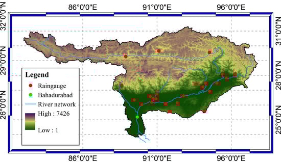
Figure 1.
Topographic map of Brahmaputra Basin along with the location of rain gauges and the outlet of the basin (Bahadurabad).
Brahmaputra River flows through Tibet (1625 km), India (918 km) and Bangladesh (363 km) for a total length of 2880 km [38]. The river has several tributaries, which differ in characteristics due to their topography, climate and land use. Generally, the flow of the river can be characterized as low flows in winter and high flows during summer due to the effect of snowmelt and monsoon rainfall. The Indian part of the basin was the main focus of the study. Accordingly, the outlet of the basin was considered at Bahadurabad (Figure 1) and the part of the basin in Bangladesh was not considered. At Bahadrudabad the annual average discharge is about 21,993 m3/s with a minimum and maximum recorded discharge values of 3280 m3/s and 102,534 m3/s [37,39,40].
The basin has a limited number of meteorological and hydrological stations. Lack of sufficient and high-quality data constrains rainfall-runoff modelling [41]. Due to the unavailability of accurate water-related models, it is difficult to study properly the water management and to identify future intervention strategies. An example of possible interventions are the proposed plans in China to divert water from Brahmaputra River to Yellow River Basin [42]. This caused tensions in India and Bangladesh. In addition, India also has plans to divert the flow within its boundaries to Ganges Basin to support agricultural activities [43]. This caused tension in Bangladesh since during the dry season the river supports demands on domestic and industrial use. The availability of a model with a proper representation of the geophysical and hydrological processes of the basin may serve as a basis to solve conflicts.
For example, Schneider et al. [44] used satellite altimetry data from CryoSat-2 for calibrating a hydraulic model of Brahmaputra River. In addition, they calibrated the cross sections derived from the digital elevation model (DEM) with water level data derived from satellite altimetry. Futter et al. [41] used PERSiST, a semi distributed dynamic rainfall-runoff modelling tool, in modelling the Upper Ganges and Brahmaputra basins. Hydro-meteorological data were gathered from governmental agencies in India and FAO. Two model setups having different complexities were proposed. Two sets of simulations were performed based on two representations of the basin: simple and complex. In the simple one, for example, Brahmaputra basin was described as a single catchment whereas in the complex one it was described by 10 catchments. The models were simulated for almost 20 years. The Nash-Sutcliffe coefficient of discharge prediction at Bahadurabad varied from 0.42 to 0.65. The models were able to replicate the timing and amount of the low flows. However, high flows were underestimated or overestimated and their time of occurrence was inaccurately predicted. The authors concluded that the complex setup performed better than the simple one. One main reason for model inaccuracies was the lack of data and the unaccounted water withdrawal in the upper part of the basin [41]. Mahanta et al. [37] reported another study conducted by the International Union for Conservation of Nature (IUCN) where a lumped, deterministic and conceptual rainfall-runoff model based on NAM and MIKE11 for routing was used. The study was carried out for the time period 2008 to 2011. The Nash Sutcliffe coefficient for discharge estimation varied from 0.75 to 0.89. Also, in this case, the short calibration and validation time periods and lack of in-situ data are seen as limitations.
3. Methodology
The main methodology proposed in this study is presented in Figure 2. Below, the different sub-sections reflect the methodological steps followed in this study. Two different approaches were used to derive flood maps. In the first (blue line in Figure 2), only freely available global datasets were used as the model forcing. In the second one (red line in Figure 2), the satellite-based rainfall data were corrected using in-situ rain gauge data and then used as model input.
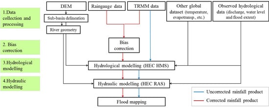
Figure 2.
Methodological approach used in this study for assessing flood extent using global data.
3.1. Data Collection and Processing
In this study, global datasets were used as the main input in developing both hydrological and hydraulic models. Table 1 presents the overview of the data used in the study. For the physical representation of the catchment and river geometry, the DEM used in this study was derived from Shuttle Radar Topography Mission (SRTM) with 90 m × 90 m resolution. Rodríguez et al. [45] have presented the accuracy of the SRTM data, which can be a concern for small basins but SRTM based DEMs have been found to be reasonably accurate in large basin [17,41,44]. Topographical information was adopted to delineate sub-basins for hydrological modelling and to derive river geometry for hydraulic modelling. The rainfall data from Multi-satellite Tropical Rainfall Measuring Mission TMPA 3B42 V7 Daily [10] was used. This gridded dataset has a resolution of 0.25° × 0.25° with a spatial coverage of 50°N–50°S. Temperature data at 2m altitude was collected from Atmospheric Infrared Sounder (AIRS) from NASA’s Earth Data Centre. In order to correct the TRMM data, 24 in-situ rain gauges covering a period of 2 years (2013 and 2014) were used. Figure 1 shows the rain gauge stations and the outlet of the basin.

Table 1.
List of data used in the study.
Additional global datasets were also used for hydrological modelling. Land use values from the Globcover dataset of the European Space Agency were used. Soil properties were extracted from FAO’s Harmonized World Soil Database (HWSD). Lithological data were based on the Global Lithographic Map (GLIM) [46]. Soil properties such as infiltration rates were estimated using the results of Bell et al. [47]. Evapotranspiration data were retrieved from the Geo Network portal of FAO. The accuracy of global datasets varies with the spatio-temporal scale and this may have an influence on the accuracy of the hydrological and hydraulic models. Bell and Kundu [48], Kundu and Bell [49] and Omranian and Sharif [50] have shown that accuracy increases with increasing spatial and temporal scales of the global datasets.
Discharge and water level were used to calibrate and validate the hydrological and hydraulic models, respectively. In particular, discharge data at the outlet of the basin for the period 2000–2015 was used to calibrate and validate the hydrological model. On the other hand, water level at the outlet was used to calibrate the hydraulic model whereas water level estimates from Jason2 altimetry data (http://www.theia-land.fr/) was used to validate the hydraulic model. Finally, inundation images from the Dartmouth Flood Observatory of the Colorado University of two flood events on 19 June 2012 and 23 September 2012 were used to validate the flood inundation model.
3.2. Bias Correction for Satellite Rainfall Estimates
Due to the fact that satellite borne rainfall measuring instruments estimate rainfall based on the column of atmosphere and not on the actual rain at the ground surface, these estimates are accompanied with retrieval errors. Correction of satellite-based rainfall estimates using gauge rainfall data, known as bias correction, is an effective way of reducing errors in the data. Bias correction of satellite-based rainfall estimates is a very active research area with many publications pointing out the usefulness of different methods in different catchments. For example, Bell and Kundu [48] and Kundu and Bell [49] presented with the help of a spectral model the variation of error between TRMM and gauge rainfall with the increasing spatial and temporal scale.
Among numerous bias correction methods arguably the Ratio Bias Correction (RBC) and Quantile Mapping are the most widely used. In RBC the correction coefficient is computed based on the average daily gauge rainfall and satellite based daily rainfall estimates over a season, month or week, which is used in correcting the daily satellite-based rainfall estimates (see Equation (1)).
where Rf,x,y represents the ratio bias correction factor for location x and season y, Pg,x,y and Ps,x,y are the daily in-situ gauge (used as reference) and remote sensing (TRMM in our study) rainfall at location x for season y, i = 1,2,…, n and n is the number of days in a season. Based on the historical data of sufficient length for both datasets the correction factors can be computed for a chosen temporal scale, for example, monthly, leading to deriving twelve correction factors. Additionally, spatial zones may be considered and the correction factors for each zone may be separately computed. These factors may subsequently be used in correcting satellite-based rainfall estimates by assuming that the computed bias for the selected spatial and temporal scale remains applicable in the future. Arial-Hidalgo et al. [14] presented the RBC method with monthly bias correction factors to improve the TRMM data for the Vinces basin in Ecuador. This method works reasonably well provided both rainfall data of sufficiently long time duration are available. On the other hand, the quantile mapping method works on finding the gauge rainfall, which has the same probability of a particular satellite-based rainfall estimate.
Gauge rainfall data from 24 stations for a period of 2 years (2013 and 2014) were only available (Figure 1). The RBC method was used with the gauge rainfall for 2013 for finding the correction factors (using Equation (1)) for TRMM rainfall for the sub-basins having a gauging station inside the sub-basin. The computed factors were used in correcting the TRMM rainfall for 2014 and were validated by comparing the corrected TRMM rainfall estimates of 2014 with the gauge rainfall. The correction factors were subsequently used in correcting the TRMM rainfall time series. The TRMM rainfall was not corrected for the other basins for which no gauge rainfall was available. Hughes and Gray [51] presented an interesting approach of correcting TRMM rainfall using hydrological information at the outlet of the basin where no gauge rainfall is available. However, such an approach requires further investigation as Brahmaputra is a much larger catchment compared to the Okavango River basin considered by the authors. Certainly, the use of gauge rainfall data of limited time period to correct TRMM data is an approximate one and we recommend that more gauge rainfall should be used in the future in the bias correction.
3.3. Hydrological Modelling
There were many challenges to the hydrological modelling of the Brahmaputra basin due to the large variations in the physiographic and hydro-climatic properties such as elevation, land cover, soil characteristics, rainfall and temperature. An additional challenge was related to the limited availability of hydro-meteorological data. The purpose of the model was to adequately simulate the catchment hydrology with the main focus on the surface water resources.
In this study, a semi-distributed hydrological model in which each sub-basin is represented as a lumped model was implemented. The widely used HEC-HMS model (http://www.hec.usace.army.mil/software/hec-hms/) was chosen. The catchment was delineated and the river network was identified using the SRTM data in a GIS environment with Bahadurabad (Figure 1) as the outlet of the catchment. Bahadurabad was chosen as discharge data were available at that location. The basin was sub-divided into 39 sub-basins. The land use information was extracted in a GIS environment from the Globcover data. Similarly, the soil data was derived from the HWSD data. Specific catchment properties such as infiltration rate, percolation rate and so forth were derived from the lithological information following the recommendation of Bell et al. [47].
The hydrological processes in the catchment were modelled using Soil Moisture Accounting (SMA) model to simulate the precipitation loss, Clark Unit Hydrograph to simulate the direct runoff and Linear Reservoir to model the baseflow. SMA was used as it is very suitable for hydrological simulation of wet and dry periods over a long period of time. The SMA consisted of five linear reservoirs: canopy, simple surface, soil storage, groundwater-1 and groundwater-2. The canopy interception was modelled with Simple Canopy method with maximum storage capacity varying from sub-basin to sub-basin from 1 to 5 mm. The maximum storage capacity was considered as 1 mm for the upstream barren sub-basins and was gradually increased to 5 mm for the forested sub-basins. The initial canopy storage was considered as zero as the initial values do not influence the simulation after a few weeks/ months of simulation. Storage in surface depressions was modelled using Simple Surface method with maximum storage capacity varying from sub-basin to sub-basin from 7 to 9 mm depending upon their terrain. The initial storage was considered as zero.
HMS allows representing groundwater in two storages, Groundwater 1 and 2. Together with the Soil Storage they form the main storages of water in the model. The flow to the Soil Storage is primarily determined by the infiltration capacity and to the groundwater layers by percolation rates. The infiltration capacity was assessed based on the lithological properties [47] and varied from 5.1 to 20.3 mm/h. The percolation rates varied from 0.3 to 1.2 mm/h for Groundwater-1 and 0.04 to 0.25 mm/h for Groundwater-2. These values were estimated from the lithological properties of the catchment [46]. Groundwater coefficients, controlling the flow from the groundwater, were estimated as 80 to 120 hr for Groundwater-1 and 200 to 400 for Groundwater-2.
The Clark Unit Hydrograph (CUH), which was used to model the direct runoff, uses the excess rainfall computed by the SMA and converts that to direct runoff. The lag time was computed using the length of the longest flow path and the length of the stream from the point nearest to the centroid of the outlet. The time of concentration, calculated based on the lag time, varied between 56 and 128 h. The storage coefficient values, depending on the size of the catchment, varied between 5 and 12 h. In the linear reservoir, which was used to simulate the baseflow, the initial discharge for each catchment was computed by multiplying the measured initial discharge at the outlet (Bahadurabad) by the ratio of the respective catchment size to the total basin size. The groundwater coefficient in the baseflow model was varied depending upon the catchment size between 8 and 15 h.
The meteorological forcing was applied using two different datasets: uncorrected TRMM and corrected TRMM. The monthly average evapotranspiration data, estimated from FAO, was used. The values varied between 30 and 50 mm during the winter months, 60–80 mm during the spring months and 80–120 mm during the summer months. The Temperature Index method was used to simulate the snow melt in the upper part of the catchment.
Daily discharge information at Bahadurabad were available for the time period 1 January 2000 to 26 December 2015. The calibration period was set from 1 January 2005 to 29 April 2013. Table 2 shows the calibration and validation period for the hydrological and hydraulic models. The measured discharge at Bahadurabad was used in the calibration of the model. Unfortunately, there was no other observed discharge/water level data to calibrate the large basin model. Discharge data from April 2013 up to the end of 2015 were not used in the calibration due to the high percentage of missing data.
Table 2.
Calibration and validation period for the hydrological and hydraulic models.
The calibration of the hydrological model was carried out using an automatic procedure based on Univariate Gradient search algorithm, maximizing the Nash Sutcliffe coefficient between the simulated and observed discharge at the Bahadurabad station. The following hydrological model parameters were calibrated: SMA parameters (soil storage, GW1 and GW2 storage coefficients, maximum infiltration rates, percolation rates scale factor, GW1 and GW2 storage scale factor, tension storage scale factor), GW1 and GW2 coefficients of the linear reservoir model and storage coefficient for the Clark Unit Hydrograph. The parameter values were different among the 39 sub-basins. Because of the availability of the observed data only at the outlet and the presence of high number of model parameters, some parameters of the semi distributed model (such as percolation rates to GW1 and GW2) were calibrated using a scale factor, that is, a number between 1 and 100 (real-valued) which can be determined for a parameter during the calibration. The calibrated value of the scale factor is valid for the chosen parameter for the entire basin. The calibrated scale factor can then be used to multiply the initial values of the chosen parameter of each sub-basin to obtain the calibrated parameter values. For other parameters, this constraint was not imposed. This may not be the ideal way of optimising model parameters when the measured data over a long period of time at a number of locations is available.
Using the optimized parameters, the model was simulated for the validation period 1 January 2000 to 31 December 2004 with a daily time step. It is worth noting that model calibration and validation are extremely dependent to the availability and accuracy of flow data.
3.4. Hydraulic Modelling
For the hydraulic modelling, the last 500 km of the river ending at Bahadurabad was chosen as the model domain (see Figure 3). The particular choice was due to the availability of water level/discharge data at Bahadurabad and the presence of some important urban settlements, including the provincial capital Guwahati, in the region. HEC-RAS (version 5) and HEC-GeoRAS (version 10.2) from the Hydrologic Engineering Centre (HEC) of the US Army Corps of Engineers were used. Because of the unavailability of observed river cross sections for the studied 500 km river reach, the geometry data was processed in the GIS environment using the SRTM 90 m × 90 m as the topographic information. The centreline of the river, flow paths, riverbanks, bed slopes, reach lengths, river cross sections (every 500 m) and river floodplain were generated from the SRTM DEM using GIS-based approaches implemented in the HEC GeoRAS toolbox. No other correction was made for the vegetation and to the river bathymetry in the cross sections of the main channel. Domeneghetti [52] has presented techniques for estimating river geometry data in data-scarce regions while Baugh et al. [53] have presented procedures to correct for vegetation while extracting geometry data from SRTM. In our research we had no primary geometry data to cross-check the suitability of these methods in this large basin and as a result, we recommend exploring these approaches in future research. If measured cross-sections (perhaps limited in numbers) are available then the extracted cross-sections should be compared and if needed, they should be corrected. In this research no measured geometry data was available. The processed geometry data was imported in the HEC-RAS environment. In addition, the channel width was compared to the one estimated using Google Earth image and functions.
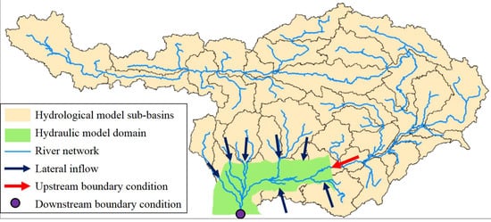
Figure 3.
Representation of the sub-basins of the hydrological model and the domain of the hydraulic model (last 500 km of the river). Outflow from the hydrological model are considered both as lateral inflow (from 8 sub-basins) and upstream boundary condition (inflow contribution from 31 sub-basins) to the hydraulic model.
The downstream part of the basin ending at Bahadurabad was chosen as the domain of the hydraulic model. For this reason, the discharge data simulated with the hydrological model HEC-HMS was used as the upstream boundary condition for the hydraulic model, while the normal depth was chosen as the downstream boundary condition. Simulated flows from the sub-basins and tributaries (from the hydrological model) corresponded to the lateral inflows to the hydraulic model domain (see Figure 3). More details on the calibration and validation periods of both hydrological and hydraulic model are reported in Table 2.
In order to calibrate the hydraulic model, different values of the Manning’s roughness coefficient for the floodplain nfp (0.035, 0.025 and 0.02) and main channel nch (0.03, 0.02 and 0.015) were used. The model was then calibrated by changing Manning’s roughness coefficient by comparing the simulated and observed water levels at Bahadurabad. The calibrated Manning’s roughness parameter values of the hydraulic model were 0.025 for floodplains and 0.02 for the main channel, which agreed with the values reported in the literature (see, for example, Jung et al. [54] and Fisher et al. [55]). The hydraulic model was validated with the water level estimated from Jason-2 satellite (see, for example, the Hydroweb portal http://www.theia-land.fr/en).
The validation period was chosen based on the availability of remote sensing images of flood events in those specified periods. Due to the lack of measured water level/discharge data inside the basin the water level estimated from satellite altimetry (JASON-2) was used in validating the hydraulic model. Satellite altimetry has been useful in various studies with limited or no gauging stations (e.g., Papa et al. [56] and Yan et al. [57]). Jason-2 satellite has a virtual observation point in Brahmaputra River, which happens to be inside the domain of our hydraulic model. The frequency of satellite pass is 10 days. Water levels from Jason-2 for the year 2015 was used in validating the hydraulic model.
3.5. Performance Indices
The flood extent maps developed with the hydraulic model were compared with flood inundation maps from observed flood extent data to investigate model performances. Simulated flood extent maps were generated by interpolation of simulated water levels between cross sections considering an area flooded when the water level was higher than 0.1 m. Inundation images from the Dartmouth Flood Observatory of the Colorado University were used as observed flood extent. As there was no measured flood depth and flood extent data available, the accuracy of the satellite image was not checked. Flood maps information were downloaded as polygons for the 2 selected flood events and then converted as flood extent maps having the same spatial resolution of the simulated flood extent maps, that is, 90 m × 90 m.
The accuracy of the simulated flood maps was evaluated using the Critical Success Index (CSI), which is frequently used in estimating the accuracy of flood forecasts [58,59,60,61,62]. In particular the following indices were derived: Probability of Detection (POD, shows what flood fraction of the observed events was correctly simulated), False Alarm Ratio (FAR, shows what dry fraction of the flood event was incorrectly simulated as flooded) and Critical Success Index (CSI, is an indication of the goodness of fit between the simulated and observed flood). Separate binary maps were created from the simulated flood inundation maps and observed imageries with each pixel having a value [1,2] where 1 denotes no flood at the pixel and 2 denotes flooding at the pixel. Equation (2) illustrates the CSI indices.
where A is the false alarm (meaning that observed pixel in the observed flood extent image is dry and simulated pixel is wet), B is the correct alarm (meaning that both observed and simulated pixels are wet) and C is the missed alarm (meaning that observed pixel is wet and simulated pixel is dry). The closer to one the values of CSI and POD are, more accurate the model is. An opposite consideration can be drawn for FAR.
Two flood events were chosen for the validation of the developed flood maps: (1) Event-1 on 29 June 2012 and (2) Event-2 on 23 September 2012. The observed maximum discharges at Bahadurabad during these two flood events were 97,824 and 97,500 m3/s respectively whereas the maximum observed discharge at Bahadurabad during the simulation period (2000–2015) was 102,585 m3/s. On both these extreme events, the basin was affected by large flooded area and severe damages. Moreover, we chose these flood events for validating our methodology because of the availability of flood extent satellite images.
While this paper presents the use of remote sensing information in hydrological and hydraulic models to generate flood maps, another possible solution exists in extracting flood information using geomorphic DEM-based approach that refers only to the topographic information. For example, Manfreda et al. [63] used topographic index based on catchment morphological characteristics to identify flood-prone areas of the Upper Tiber River in Italy.
4. Results and Discussion
4.1. Bias Correction
Figure 4a shows the annual average rainfall based on uncorrected TRMM for each catchment for 2014 of and Figure 4b shows the same with the corrected TRMM. We observed an increase in annual average rainfall on areas in the Himalayan slopes. The increase ranged from 10% to 114%. This corroborated with the findings of previous studies that TRMM usually underestimates more intense rains (Arias-Hidalgo et al. [14]). By correcting, we increased the magnitude of satellite-based rainfall estimates. On the other hand, the correction led to reduced rainfall amount in areas with low annual rainfall. The decrease ranged from 9% to 42%. The corrections perhaps could not remove all the errors. The RBC method for bias correction uses daily correction factor for each month or season, which works well when both the gauge and satellite-based rainfall estimates are available for a long period of time. The corrections applied here were based on data of one year. The correction factors varied from 0.18 to 2.42. Higher values were obtained for the wet months. The correction factors also varied spatially. Higher correction factors were observed in the Himalayan slopes. We hope that in the future longer period of gauge rainfall will be available to further improve the correction of the TRMM data. If longer time series of gauge rainfall data is available then more widely used probabilistic method Quantile Mapping [14] can be used. Another alternative to this method will be to use the discharge data at the outlet to correct the TRMM rainfall data [50], which however, is suitable only for small basins.
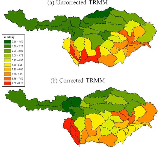
Figure 4.
(a) Uncorrected and (b) corrected annual average TRMM rainfall for 2014 over different sub-catchments of the Brahmaputra basin.
4.2. Hydrological and Hydraulic Modelling
Figure 5 shows the comparison of simulated and observed discharge values for the calibration and validation period respectively using uncorrected and corrected TRMM data. In general, the trend of the discharge data has been followed reasonably well in both simulations. As expected, model forced by corrected TRMM data provided relatively better results (especially during peaks) than the ones obtained with uncorrected rainfall data. However, simulated discharge with the uncorrected forcing showed a similar trend achieved using corrected input. Table 3 presents the analysis of model’s accuracy for the calibration and validation data using both the corrected and uncorrected TRMM data. For the calibration period the Nash Sutcliffe Coefficient (NSC) of 0.75 with an R2 of 0.8 and root mean square error (RMSE) 9625 m3/s was obtained using uncorrected TRMM data. When the corrected TRMM data was used the NSC, R2 and RMSE values were 0.81, 0.81 and 7272 m3/s, respectively. The low flow values could not be properly represented in both simulations. This can be due to the complex nature of the hydrological phenomena in the catchment and to the simplified structure of the model itself. The differences might have originated also from the imprecise rainfall information from TRMM. Note that limited gauge data was used in correcting the TRMM rainfall. Moreover, the model was calibrated only with the discharge data at the outlet, which might have resulted in uncertain model parameters. It has been shown that TRMM is able to represent low and heavy rainfall but still significantly underestimate magnitude of rainfall, particularly in orographically influenced areas [64].
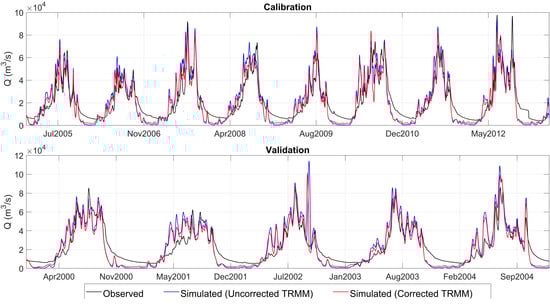
Figure 5.
Comparison of the simulated (using uncorrected and corrected TRMM products) and observed hydrograph at Bahadurabad for the calibration (first row) and validation (second row) periods.
Table 3.
Analysis of accuracy of the hydrological model over the calibration and validation period with the uncorrected and corrected TRMM data.
Although some differences are discernible it is noteworthy that the focus of the research was on producing flood maps using remote sensing data in large scale sparsely gauged basins. Due to data limitation, it is not unlikely to have differences in modelling results, for example, in base flows. It is important to note that the discharge time series was predicted reasonably well. The flood maps produced with the simulated discharge data (shown in the following section) showed reasonably good accuracy.
Related publications [14,36], present reasonably good fit between observed discharge and discharge simulated with TRMM rainfall though differences with measured discharge, particularly during the low flows, are discernible. The differences, as have been mentioned before, are mostly due to imprecise rainfall data, uncertain model parameters and semi-distributed modelling approach, which embodies a limited representation of the hydro-geomorphological processes occurring in the catchment. Researchers are globally active on improving hydrological modelling with imprecise remote sensing products. At the same time, it is noteworthy that there is an urgent need of providing model-based information of sparsely gauged catchments.
For the validation period NSC, R2 and RMSE values with the uncorrected and corrected TRMM data were 0.61, 0.77, 11,643 m3/s and 0.74, 0.79 and 9201 m3/s, respectively. This justifies the use of the corrected TRMM data. The magnitude and timing of the peaks were replicated well. Although the simulation results with the corrected TRMM data were better than the ones with the uncorrected TRMM it is noteworthy that the results with the uncorrected TRMM were similar to the simulation results with the corrected TRMM data. This justified the use of uncorrected global datasets in hydrological simulations of the basin.
Figure 6 presents the comparison between the water level simulated (with uncorrected and corrected TRMM data) by the hydraulic model for the period 01/Jan/2013 to 31/Dec/2013 (calibration) at Bahadurabad with the measured water level. Figure 6 also presents the validation of the hydraulic model for the period 01/Jan/2015 to 26/Dec/2015 for the location near Barpeta with the water level data estimated from Jason-2. The measured water level was unavailable for several months of 2013 and the initial differences with the simulated water levels can be attributed to the warming up of the model. Note that for the validation period the simulated and observed water levels have two different time steps. In particular, simulated water levels were available for every day whereas the water level estimated from the radar altimetry was available once every 10 days. In general, comparable accuracy was achieved using both uncorrected and corrected model forcing, showing reasonably good agreement with the water level estimated from Jason-2. However, we observed some discrepancies between model and observed results on low flows and early start of the rainy season. For the period of low flows during the month of February and March the simulated water level was lower than the observed water level while for the month of April and May the simulated water level was higher than the observed water level. This phenomenon corresponds to the same situation on the discharges of the hydrological model. The difference of water level ranged from 0.50 m to 1.0 m. Nonetheless, the results were encouraging and they proved the usefulness of using uncorrected global datasets for the estimation of water level in the scarcely gauged large-scale Brahmaputra catchment.
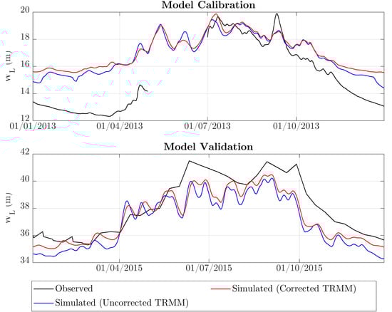
Figure 6.
Top: Calibration of the hydraulic model by comparing the water level simulated by the hydraulic model with the water level measured at Bahadurabad. Bottom: Validation of the hydraulic model by comparing the water level simulated by the hydraulic model with the water level estimated from Jason-2 for 2015 for the location near Barpeta.
4.3. Flood Extent Results
For flood Event-1 on 29 June 2012 the observed discharge at Bahadurabad gauging station was 97,824 m3/s while for the flood Event-2 on 23 September 2012 the observed discharge was 97,500 m3/s. The hydraulic model was used to simulate the 2 selected flood events for the purpose of flood mapping. HEC-GeoRAS can post-process output of HEC-RAS. Maximum water surface profiles from HEC-RAS were converted into a GIS spatial dataset using HEC-GeoRAS [65]. Flood maps were then generated for the 2 selected flood events using HEC-GeoRAS. Figure 7 shows the generated flood map for Event-2 with the uncorrected TRMM data.
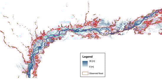
Figure 7.
Simulated (using uncorrected TRMM) and satellite observed inundation map for the flood of 23 September 2012.
The flood inundation maps were compared with satellite images. The source of satellite observed flood maps was Dartmouth Flood Observatory [66]. Figure 7 presents a visual comparison with the simulated inundation map for Event-2. Overall, there is a good agreement between the simulated results and the observed flood extent. In particular, a good fit between the observed and simulated flood extent is achieved in the downstream part of the 500 km reach of the river. On the contrary, the model tends to overestimate flood extent in the upstream part. This could be related to the error in the interpolation of cross-sections (every 500 m) for assessing flood extent and in the errors in the river geometry extractions using SRTM data. It is worth noting that this information could be affected by different sources of error. Indeed, flood extent maps derived from remote sensing images suffer from over- and under-detection as well, due for instance to dry pixel with radiometry similar to the one of open water or objects masking water (“blind spots” due to vegetation and buildings). In particular, one issue in the downstream area of the Brahmaputra catchment (domain of the hydraulic model) could be the presence vegetation masking water which could lead to an underestimation of the flood extent [67]. Furthermore, it is also noteworthy that the simulation accuracy of the hydrological model directly affects flood inundation results. If the hydrological model under-predicts discharge then less inundation in the hydraulic modelling results may be observed and on the other hand if the hydrological model over-predicts discharge then larger inundation in the hydraulic modelling results may be noticed. Such an analysis is possible if measured discharge at more locations inside the basin is available. As this data was not available, this analysis was not carried out.
To further compare the simulated flood maps with the satellite-based flood maps, we estimated the parameter values for positive rejection, false alarms, hits and misses following the procedure presented in Section 3.5. The results of this analysis are shown in Figure 8 and it can be observed that both for the uncorrected and corrected TRMM a good hit rate is obtained, followed by a considerable number of false alarm areas. In particular, results obtained using uncorrected and corrected TRMM data show comparable results. However, it appears that the uncorrected TRMM tends to provide more missed alarms in the central and upper part of the 500 km river reach, while the corrected TRMM shows high false alarm areas in the downstream section of the reach. Results are encouraging considering the simplified hydraulic modelling set up. A more detailed analysis is provided in the next section.
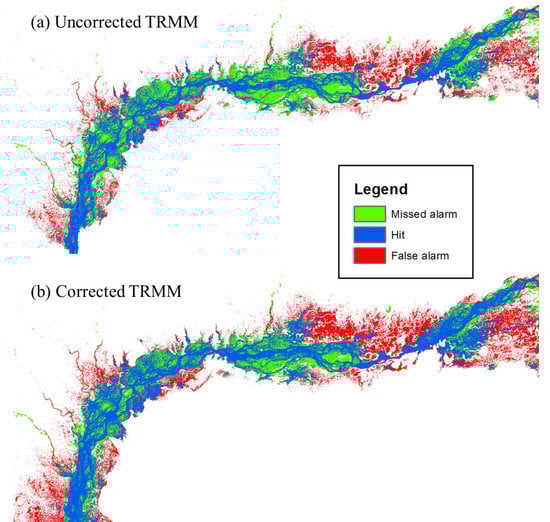
Figure 8.
Comparison between hit, missed alarm and false alarm for the flood of 23 September 2012.
As the catchment is rather large we considered some specific areas where the performance of the hydraulic model was further evaluated. In particular, the following three urban settlements were considered: Guwahati, Barpeta and Dhubri. These cities are among the important ones in the basin. Guwahati is the provincial capital and the most important city in this part of India. The administrative boundaries of the cities are shown in Figure 9. The three cities are on one side of the river and some of their areas are far from the river which are unlikely to be flooded. Due to this reason three rectangular areas covering both sides of the river were chosen as well. They are named as Upper Zone, Middle Zone and Lower Zone in Figure 9 and are located in the upper, middle and lower part of the basin, respectively. The performance indices A, B and C (Equation (2)) were computed for each of the above-mentioned zones using the simulated map and the satellite image.
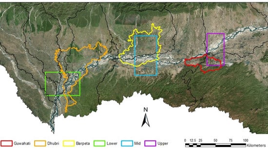
Figure 9.
Considered areas for the evaluation of the hydraulic model results.
As reported above, positive rejection, false alarms, hits and misses were computed for the six identified zones for the two flood events and are shown in percentages of the total pixels in Table 4 and Table 5. Both flood events (Table 4 and Table 5) show comparable results. The cumulative values for positive rejections and hits (meaning the model was correct) varied with the corrected TRMM between 71% and 87%, which was considered as reasonably high given the fact that very little ground data was used in the research. The cumulative values for positive rejections and hits with the uncorrected TRMM varied between 68% and 89%. The false alarm ratio with the corrected TRMM varied between 5% and 20% whereas with the uncorrected TRMM it varied between 4% and 17%. Due to the low resolution of the DEM used in the research some of the protection infrastructures might not have been represented in the model and as a result some pixels could have been simulated as flooded whereas in reality they were dry as they were protected. The satellite image captured the real flood extent whereas the simulated flood map was influenced by the lack of presence of the flood protection structures (limited presence only around large urban settlements) in the DEM. The missed alarm ratio with the corrected TRMM varied between 1% and 18% whereas with the uncorrected TRMM data it varied between 1% and 24%. The missed alarm ratio (with the corrected TRMM data) was really low for Guwahati (1%) but was high for other locations (up to ~18%). There was no obvious explanation behind it though we anticipate that the relatively high false alarm ratio contributed to a relatively high missed alarm. It is noteworthy from Table 4 and Table 5 that the positive rejection, hit, false alarm and missed alarm values with the uncorrected TRMM data for all the locations were very close to the values obtained with the corrected TRMM data.
Table 4.
Contingency table for the flood event of 23-09-2012. The numbers show the percentage of pixels of inundation maps falling into the four groups: positive rejection, false alarm, missed alarm and hits for the six chosen geographic locations.
Table 5.
Contingency table for the flood event of 29-06-2012. The numbers show the percentage of pixels of inundation maps falling into the four groups positive rejection, false alarm, missed alarm and hits for the six chosen geographic locations.
Subsequently, the POD, FAR and CSI indices were computed for the two flood events (see Section 3.5). It may be noted that a higher value of POD indicates larger number of grid cells, which are observed in the satellite image as flooded are also simulated as flooded (indicating good model performances). A lower value of FAR indicates smaller number of grid cells, which are observed in the satellite image as not flooded are identified as flooded in the simulation. The prediction skills are indicated by the CSI and a higher value indicates more grid cells are correctly identified as flooded or not flooded. As can be seen from Figure 10 the indices are comparable for both events. Overall, slightly better model performances are achieved (as expected) using the corrected TRMM. However, CSI values during the event in June 2012 (Event-1) are higher using uncorrected TRMM in Barpeta, Dhubri and the middle part of the river reach. For the event of September 2012 (Event-2) the indices obtained using the corrected TRMM are generally higher than the ones achieved with the uncorrected TRMM in all the 6 considered regions. It is also noticed that performance indices are generally higher during Event-1. This can be partly explained from the fact that the simulated discharge when compared to the observed discharge for Event-2 had larger error compared to that of Event-1. For Event-2 the simulated discharges at the chosen locations were less than actual and for that reason POD is less. Lower values of FAR for Event-2 can also be justified by this explanation. Therefore, the relatively low accuracy of the simulated inundation map for Event-2 was due to larger simulation errors in the hydrological model.
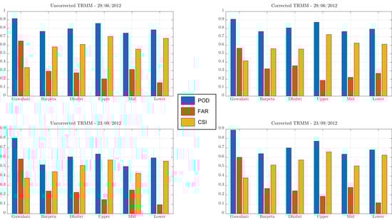
Figure 10.
Performance coefficients assessed comparing simulated and observed flood extent in the six considered areas along the river during the two considered flood events with the uncorrected and corrected TRMM data.
It is worth noting that for all flood events the Guwahati area had high accuracy (Figure 10). Generally, the model produced good results. POD values were mostly above 0.80, FAR was also high with values above 0.80 and CSI values were above 0.75.
5. Limitations and Recommendations
One of the limitations of this study is the limited availability and poorly distributed rain gauge data, so only a minimal bias correction of the satellite-based rainfall data was carried out. The calibration of the hydrological model was based only on the discharge at the outlet. The semi-distributed nature of the hydrological model, which embodies a limited representation of the hydro-geomorphological processes occurring in the catchment, imprecise rainfall data (from TRMM) and inadequate calibration data contributed to modelling errors. Moreover, more advanced hydrological models which optimize topographic information such as WFIUH (Petroselli and Grimaldi [68]) should be used as well.
The hydraulic modelling was carried out using the 1D method and lateral propagation of the flood was not considered. This limitation is particularly important in shallow areas like the floodplain of the Brahmaputra River. Additional studies using coupled 1D-2D or fully 2D models are required to further validate our conclusion. Since river geometry is the main driving information in hydraulic modelling [67], more detailed information regarding channel and floodplain geometries should be included in future studies. More detailed cross sections should be used in hydraulic modelling as the ones used in this study were based on the SRTM data and there are limitations in estimating river bathymetry from SRTM data.
6. Conclusions
Global datasets based on remote sensing products can provide useful information in data scarce basins. The aim of this study was to demonstrate the usefulness of remote sensing information to carry out flood modelling in a data scarce area such as the Brahmaputra basin. For this reason, different remote sensing products providing hydro-meteorological information were used for building, calibrating and validating the hydrological and hydraulic models. The authors decided to adopt a coupled hydrological and hydraulic modelling framework because it allows to simulate and predict flood extents at different scales as demonstrated by different studies (e.g., [34,35,69]). Two different sets of precipitation input (TRMM and TRMM corrected using bias correction) were used. The hydrological and hydraulic models were calibrated by comparing model results with the observed data at Bahadurabad Station. The simulated flood extents were compared with satellite images for two different flood events.
This study demonstrated that remote sensing information can help to properly simulate flood extent if integrated in a cascade of hydrological and hydraulic models. Improved model results are obtained when bias correction is applied to TRMM data. In particular, the hydrological model results were able to correctly represent peaks and timing of the flood. However, during low flows in the months of February and March, simulated discharges were lower than the observed values.
Considering the simplified hydraulic modelling set up the results obtained were satisfactory. A good agreement between simulated and satellite observed water levels, further demonstrating the effectiveness of using remote sensing data in hydraulic modelling for Brahmaputra basin. Flood maps were also generated from the simulation of two flood events. Simulated flood inundation maps were compared with the satellite observed flood maps. Very good similarity was observed between the simulated and observed maps. However, it was also observed that the simulated flood maps tend to overestimate the observed flood mainly in shallow areas. Possible explanations could be that the presence of flood protection structures was not properly represented in the low resolution of the DEM. A more detailed analysis was performed on six different regions within the Brahmaputra River. This analysis showed very good match between simulated and observed maps. In particular, we got results with values of POD, FAR and CSI index higher than 0.75 in all the six regions. Results obtained with the uncorrected TRMM data and corrected TRMM data were comparable. The results of our study proved that remote sensing information can be used for hydrological and hydraulic modelling to correctly determine areas which are prone to flooding and subsequently be used in flood risk management. In addition to model calibration and validation, remote sensing products of water level could be also used in data assimilation application for properly updating model states and/or parameters and improve model forecasting near-real time as recently demonstrated by Hostache et al. [69] and Wood et al. [70]. Assimilation of remote sensing of water level in hydraulic models is a non-trivial problem which is receiving growing attention in the last years.
Author Contributions
Contributions of each author: Conceptualization: B.B. and M.M.; Methodology: B.B., M.M. and R.U.; Use of hydrological modelling Software: R.U. and B.B.; Use of hydraulic modelling Software: R.U. and M.M.; Validation, R.U., B.B. and M.M.
Funding
This research received no external funding.
Conflicts of Interest
The authors declare no conflict of interest.
References
- Kummerow, C.; Barnes, W.; Kozu, T.; Shiue, J.; Simpson, J. The Tropical Rainfall Measuring Mission (TRMM) sensor package. J. Atmos. Oceanic Technol. 1998, 15, 809–817. [Google Scholar] [CrossRef]
- Huffman, G.; Bolvin, D.; Nelkin, E.; Wolff, D.; Adler, R.; Gu, G. The TRMM Multisatellite Precipitation Analysis (TMPA): Quasi-global, multilayer, combined-sensor precipitation estimates at fine scales. J. Hydrom. 2007, 8, 38–55. [Google Scholar] [CrossRef]
- Prasetia, R.; As-syakur, A.R.; Osawa, T. Validation of TRMM precipitation radar satellite data over Indonesian region. Theor. Appl. Climatol. 2013, 112, 575–587. [Google Scholar] [CrossRef]
- Kneis, D.; Chatterjee, C.; Singh, R. Evaluation of TRMM rainfall estimates over large Indian river basin (Mahanadi). Hydrol. Earth Syst. Sci. 2014, 18, 2502–2943. [Google Scholar] [CrossRef]
- Peng, B.; Shi, J.; Ni-Meister, W.; Zhao, T.; Ji, D. Evaluation of TRMM Multisatellite Precipitation Analysis (TMPA) products and their potential hydrological application at an arid and semiarid basin in China. IEEE J. Sel. Top. Appl. Earth Obs. Remote Sens. 2014, 7, 3915–3930. [Google Scholar] [CrossRef]
- Yong, B.; Chen, B.; Gourley, J.J.; Ren, L.; Hong, Y.; Chen, X.; Wang, W.; Chen, S.; Gong, L. Intercomparison of the Version 6 and Version 7 TMPA precipitation products over high and low latitudes basins with independent gauge networks: Is the newer version better in both real-time and post-real-time analysis for water resources and hydrologic extremes? J. Hydrol. 2014, 508, 77–87. [Google Scholar]
- Cai, Y.; Jin, C.; Wang, A.; Guan, D.; Wu, J.; Yuan, F.; Xu, L. Spatial-temporal analysis of the accuracy of Tropical Multisatellite Precipitation Analysis 3B42 precipitation data in mid-high latitudes of China. PLoS ONE 2015, 10, e0120026. [Google Scholar]
- Chen, S.; Hu, J.; Zhang, Z.; Behrangi, A.; Hong, Y.; Gebregiorgis, A.S.; Cao, J.; Hu, B.; Xue, X.; Zhang, X. Hydrologic evaluation of the TRMM multisatellite precipitation analysis over Ganjiang Basin in humid south-eastern China. IEEE J. Sel. Top. Appl. Earth Obs. Remote Sens. 2015, 3, 4568–4580. [Google Scholar] [CrossRef]
- Cai, Y.; Jin, C.; Wang, A.; Guan, D.; Wu, J.; Yuan, F.; Xu, L. Comprehensive precipitation evaluation of TRMM 3B42 with dense rain gauge networks in amid-latitude basin, northeast, China. Theo. Appl. Climatol. 2016, 126, 659–671. [Google Scholar] [CrossRef]
- Kumar, D.; Gautam, A.K.; Palmate, S.S.; Pandey, A.; Suryavanshi, S.; Rathore, N. Evaluation of TRMM multi-satellite precipitation analysis (TMPA) against terrestrial measurement over humid sub-tropical basin, India. Theo. Appl. Climatol. 2017, 129, 783–799. [Google Scholar] [CrossRef]
- Ochoa, A.; Pineda, L.; Crespo, P.; Willems, P. Evaluation of TRMM 3B42 precipitation estimates and WRF retrospective precipitation simulation over the Pacific-Andean region of Ecuador and Peru. Hydrol. Earth Syst. Sci. 2014, 18, 3179–3193. [Google Scholar] [CrossRef]
- Liao, L.; Meneghini, R. Validation of TRMM precipitation radar through comparison of its multi-year measurements to ground-based radar. J. Appl. Meterol. Climatol. 2009, 48, 804–817. [Google Scholar] [CrossRef]
- Rozante, J.R.; Moreira, D.S.; De Goncalves, L.G.; Vila, D.A. Combining TRMM and surface observations of precipitation: Technique and validation over South America. Am. Meteorol. Soc. 2010, 25, 885–894. [Google Scholar] [CrossRef]
- Arias-Hidalgo, M.; Bhattacharya, B.; Mynett, A.E.; Griensven, A.V. Experience in using the TMPA-3B42R satellite data to compliment rain gauge measurements in the Ecuadorian coastal foothills. Hydrol. Earth Syst. Sci. 2013, 17, 2905–2915. [Google Scholar] [CrossRef]
- Joyce, R.; Janowiak, J.E.; Arkin, P.A.; Xie, P. CMORPH: A method that produces global precipitation estimates from passive microwave and infrared data at high spatial and temporal resolution. J. Hydrometeorol. 2004, 5, 487–503. [Google Scholar] [CrossRef]
- Hsu, K.-L.; Gao, X.; Sorooshian, S.; Gupta, H.V. Precipitation estimation from remotely sensed information using artificial neural networks. J. Appl. Meteorol. 1997, 36, 1176–1190. [Google Scholar] [CrossRef]
- Collischonn, B.; Collischonn, W.; Tucci, C.M. Daily hydrological modelling in the Amazon basin using TRMM rainfall estimates. J. Hydrol. 2008, 360, 207–216. [Google Scholar] [CrossRef]
- Gu, H.; Yu, Z.; Yang, C.; Ju, Q.; Lu, B.-J.; Liang, C. Hydrological assessment of TRMM rainfall data over Yangtze River Basin. Water Sci. Eng. 2010, 3, 418–430. [Google Scholar]
- Xue, X.; Hong, Y.; Limaye, A.S.; Gourley, J.J.; Huffman, G.J.; Khan, I.K.; Dorji, C.; Chen, S. Statistical and hydrological evaluation of TRMM-based Multi-satellite Precipitation Analysis over the Wangchu Basin of Bhutan: Are the latest satellite precipitation products 3B42V7 ready for use in ungauged basins? J. Hydrol. 2013, 499, 91–99. [Google Scholar] [CrossRef]
- Li, Z.; Yang, D.; Gao, B.; Jiao, Y.; Hong, Y.; Xu, T. Multiscale hydrologic applications of the latest satellite precipitation products in the Yangtze River Basin using a distributed hydrologic model. J. Hydrometeorol. 2015, 16, 407–426. [Google Scholar] [CrossRef]
- Wang, W.; Lu, H.; Yang, D.; Sothea, K.; Jiao, Y.; Gao, B.; Peng, X.; Pang, Z. Modelling hydrologic processes in the Mekong River Basin using a distributed model driven by satellite precipitation and rain gauge observations. PLoS ONE 2016, 11, e0152229. [Google Scholar] [CrossRef] [PubMed]
- He, Z.; Hu, H.; Tian, F.; Ni, G.; Hu, Q. Correcting the TRMM rainfall product for hydrological modelling in sparsely-gauged mountainous basins. Hydrol. Sci. J. 2017, 62, 306–318. [Google Scholar] [CrossRef]
- Zhao, Y.; Xie, Q.; Lu, Y.; Hu, B. Hydrological evaluation of TRMM Multisatellite Precipitation Analysis for Nanliu River in humid Southwestern China. Sci. Rep. 2017, 7, 2045–2322. [Google Scholar]
- Liu, X.; Yang, T.; Hsu, K.; Liu, C.; Sorooshian, S. Evaluating the streamflow simulation capability of PERSIANN-CDR daily rainfall products in two river basins on the Tibetan Plateau. Hydrol. Earth Syst. Sci. 2017, 21, 169–181. [Google Scholar] [CrossRef]
- Thom, V.; Khoi, D.; Linh, D. Using gridded rainfall products in simulating streamflow in a tropical catchment—A case study of the Srepok River Catchment, Vietnam. J. Hydrol. Hydromech. 2016, 65, 18–25. [Google Scholar] [CrossRef]
- Alazzy, A.A.; Lü, H.; Chen, R.; Ali, A.B.; Zhu, Y.; Su, L. Evaluation of satellite precipitation products and their potential influence on hydrological modeling over the Ganzi River Basin of the Tibetan Plateau. Adv. Meteorol. 2017, 2017, 3695285. [Google Scholar] [CrossRef]
- Bitew, M.M.; Gebremichael, M. Evaluation of satellite rainfall products through hydrologic simulation in a fully distributed hydrologic model. Water Resour. Res. 2011, 47, W06526. [Google Scholar] [CrossRef]
- Bitew, M.M.; Gebremichael, M. Assessment of satellite rainfall products for streamflow simulation in medium watersheds of the Ethiopian highlands. Hydrol. Earth Syst. Sci. 2011, 15, 1147–1155. [Google Scholar] [CrossRef]
- Moradkhani, H.; Hsu, K.; Hong, Y.; Sorooshian, S. Investigating the impact of remotely sensed precipitation and hydrologic model uncertainties on the ensemble streamflow forecasting. Geophys. Res. Lett. 2006, 33, L12401. [Google Scholar] [CrossRef]
- Xu, X.; Li, J.; Tolson, B.A. Progress in integrating remote sensing data and hydrologic modeling. Prog. Phys. Geogr. Earth Environ. 2014, 38, 464–498. [Google Scholar] [CrossRef]
- Maggioni, V.; Massari, C. On the performance of satellite precipitation products in riverine flood modeling: A review. J. Hydrol. 2018, 558, 214–224. [Google Scholar] [CrossRef]
- Schumann, G.J.-P.; Neal, J.C.; Voisin, N.; Andreadis, K.M.; Pappenberger, F.; Phanthuwongpakdee, N.; Hall, A.C.; Bates, P.D. A first large scale flood inundation forecasting model. Water Resour. Res. 2013, 49, 6248–6257. [Google Scholar] [CrossRef]
- Nguyen, P.; Thorstensen, A.; Sorooshian, S.; Hsu, K.; AghaKouchak, A. Flood forecasting and inundation mapping using HiResFlood-UCI and near-real-time satellite precipitation data: The 2008 Iowa Flood. J. Hydrometeorol. 2015, 16, 1171–1183. [Google Scholar] [CrossRef]
- Paiva, R.C.D.; Collischonn, W.; Tucci, C.E.M. Large scale hydrologic and hydrodynamic modeling using limited data and a GIS based approach. J. Hydrol. 2011, 406, 170–181. [Google Scholar] [CrossRef]
- Hoch, J.M.; Haag, A.V.; van Dam, A.; Winsemius, H.C.; van Beek, L.P.H.; Bierkens, M.F.P. Assessing the impact of hydrodynamics on large-scale flood wave propagation—A case study for the Amazon Basin. Hydrol. Earth Syst. Sci. 2017, 21, 117–132. [Google Scholar] [CrossRef]
- Yoshimoto, S.; Amarnath, G. Applications of Satellite-Based Rainfall Estimates in Flood Inundation Modeling—A Case Study in Mundeni Aru River Basin, Sri Lanka. Remote Sens. 2017, 9, 998. [Google Scholar] [CrossRef]
- Mahanta, C.; Zaman, A.M.; Shah Newaz, S.M.; Rahman, S.M.M.; Mazumdar, T.K.; Choudhury, R.; Borah, P.J.; Saikia, L. Physical Assessment of the Brahmaputra River; International Union for Conservation of Nature (IUCN), 2014; Available online: https://portals.iucn.org/library/sites/library/files/documents/2014-083.pdf (accessed on 19 April 2018).
- Banerjee, P.; Salehin, M.; Ramesh, V. Water Management Practices and Policies along Brahmaputra River Basin: India and Bangladesh; SaciWaters, 2014; Available online: http://brahmaputrariversymposium.org/wp-content/uploads/2017/09/report_12-05-2014_v16.pdf (accessed on 19 April 2018).
- Mirza, M. Three recent extreme floods in Bangladesh: A hydrological analysis. Nat. Hazards 2003, 28, 35–64. [Google Scholar] [CrossRef]
- Parua, P.K. The Ganga: Water Use in the Indian Subcontinent; Springer: Dordrecht, The Netherlands, 2010. [Google Scholar]
- Futter, M.N.; Whitehead, P. Rainfall runoff modelling of the Upper Ganga and Brahmaputra Basins using PERSiST. Environ. Sci. Process. Impacts 2015, 17, 1070–1081. [Google Scholar] [CrossRef] [PubMed]
- Christopher, M. Water Wars: The Brahmaputra River and Sino-Indian Relations; US Naval War College: New Port, RI, USA, 2013. [Google Scholar]
- Mahanta, C. Water Resources on the Northeast: State of the Knowledge Base; Indian Institute of Technology Guwahati, 2006; Available online: http://siteresources.worldbank.org/INTSAREGTOPWATRES/Resources/Background_Paper_2.pdf (accessed on 19 April 2018).
- Schneider, R.; Godiksen, P.N.; Villadsen, H.; Madsen, H.; Bauer-Gottwein, P. Application of CrySat-2 altimetry data for river analysis and modelling. Hydrol. Earth Syst. Sci. 2017, 21, 751–764. [Google Scholar] [CrossRef]
- Rodríguez, E.; Morris, C.S.; Belz, J.E.; Chapin, E.C.; Martin, J.M.; Daffer, W.; Hensley, S. An Assessment of the SRTM Topographic Products; Jet Propulsion Laboratory D-31639 (Report); NASA. Available online: https://www2.jpl.nasa.gov/srtm/SRTM_D31639.pdf (accessed on 19 April 2018).
- Hartmann, J.; Moosdorf, N. The new global lithological map database GLiM: A representation of rock properties at the Earth surface. Geochem. Geophys. Geosyst. 2012, 13, 1–37. [Google Scholar] [CrossRef]
- Bell, F.G.; Cripps, J.C.; Culshaw, M.G. A review of the engineering behaviour of soils and rocks with respect to groundwater. Eng. Geol. Spec. Pubs. 1986, 3, 1–23. [Google Scholar] [CrossRef]
- Bell, T.L.; Kundu, P.K. Comparing satellite rainfall estimates with rain gauge data: Optimal strategies suggested by a spectral model. J. Geophys. Res. 2003, 108. [Google Scholar] [CrossRef]
- Kundu, P.K.; Bell, T.L. A stochastic model of space-time variability of mesoscale rainfall: Statistics of spatial averages. Water Resour. Res. 2003, 39, SWC 1-15. [Google Scholar] [CrossRef]
- Omranian, E.; Sharif, H.O. Evaluation of the Global Precipitation Measurement (GPM) Satellite Rainfall Products over the Lower Colorado River Basin, Texas. J Am. Water Resour. Assoc. 2018, 54, 882–898. [Google Scholar] [CrossRef]
- Hughes, D.A.; Gray, R. Correcting bias in rainfall inputs to a semidistributed hydrological model using downstream flow simulation errors. Hydrol. Sci. J. 2017, 62, 2427–2439. [Google Scholar] [CrossRef]
- Domeneghetti, A. On the use of SRTM and altimetry data for flood modeling in data-sparse regions. Water Resour. Res. 2016, 52, 2901–2918. [Google Scholar] [CrossRef]
- Baugh, C.A.; Bates, P.D.; Schumann, G.; Trigg, M.A. SRTM vegetation removal and hydrodynamic modeling accuracy. Water Resour. Res. 2013, 49, 5276–5289. [Google Scholar] [CrossRef]
- Jung, H.C.; Hamski, J.; Durand, M.; Alsdorf, D.; Hossain, F.; Lee, H.; Hossain, A.K.M.A.; Hasan, K.; Khan, A.S.; Hoque, A.K.M.Z. Characterization of complex fluvial systems using remote sensing of spatial and temporal water level variations in the Amazon, Congo, and Brahmaputra river. Earth Surf. Proc. Land 2010, 35, 294–304. [Google Scholar] [CrossRef]
- Fischer, S.; Pietroń, J.; Bring, A.; Thorslund, J.; Jarsjö, J. Present to future sediment transport of the Brahmaputra River: Reducing uncertainty in predictions and management. Reg. Environ. Chang. 2017, 17, 515. [Google Scholar] [CrossRef]
- Papa, F.; Bala, S.K.; Pandey, R.K.; Durand, F.; Gopalkrishna, V.V.; Rahman, A.; Rossow, W.B. Ganga-Brahmaputra river discharge from Jason-2 radar altimetry: An update to the long term satellite-derived estimates of continental freshwater forcing flux into Bay of Bengal. J. Geophys. Res. 2012, 117, 1–13. [Google Scholar] [CrossRef]
- Yan, K.; Baldassarre, G.D.; Solomatine, D.P.; Schumann, G.J. A review of low-cost space-borne data for flood modelling: Topography, flood extent and water level. Hydrol. Process. 2015, 29, 3368–3387. [Google Scholar] [CrossRef]
- Schaefer, J.T. The critical success index as an indicator of warning skill. Weather Forecast. 1990, 5, 570–574. [Google Scholar] [CrossRef]
- Horritt, M.S.; Bates, P.D. Evaluation of 1D and 2D numerical models for predicting river flood inundation. J. Hydrol. 2002, 268, 87–99. [Google Scholar] [CrossRef]
- Bhatt, C.M.; Rao, G.S.; Diwakar, P.G.; Dadhwal, V.K. Development of flood inundation extent libraries over a range of potential flood levels: A practical framework for quick flood response, Geomatics. Nat. Hazards Risk 2017, 8, 384–401. [Google Scholar] [CrossRef]
- Wing, O.E.J.; Bates, P.D.; Sampson, C.C.; Smith, A.M.; Johnson, K.A.; Erickson, T.A. Validation of a 30 m resolution floodhazard model of the conterminousUnited States. Water Resour. Res. 2017, 53, 7968–7986. [Google Scholar] [CrossRef]
- Bernhofen, M.V.; Whyman, C.; Trigg, M.A.; Sleigh, P.A.; Smith, A.M.; Sampson, C.C.; Yamazaki, D.; Ward, P.J.; Rudari, R.; Pappenberger, F.; et al. A first collective validation of global fluvial flood models for major floods in Nigeria and Mozambique. Environ. Res. Lett. 2018, 13, 1748–9326. [Google Scholar] [CrossRef]
- Manfreda, S.; Nardi, F.; Samela, C.; Grimaldi, S.; Taramasso, A.C.; Roth, G.; Sole, A. Investigation on the Use of Geomorphic Approaches for the Delineation of Flood Prone Areas. J. Hydrol. 2014, 517, 863–876. [Google Scholar] [CrossRef]
- Bajracharya, S.R.; Palash, W.; Shrestha, M.S.; Khadgi, V.R.; Duo, C.; Das, P.J.; Dorji, C. Systematic Evaluation of Satellite-Based Rainfall Products over the Brahmaputra Basin for Hydrological Applications. Adv. Meteorol. 2015, 2015, 398687. [Google Scholar] [CrossRef]
- USACE. HEC GeoRAS GIS Tools for Support of HEC-RAS Using ArcGIS: User’s Manual; (version 4.3); US Army Corps of Engineers, 2011. Available online: http://www.hec.usace.army.mil/software/hec-georas/documentation/HEC-GeoRAS_43_Users_Manual.pdf (accessed on 19 April 2018).
- Dartmouth Flood Observatory. Retrieved from Dartmouth Flood Observatory. 2010. Available online: http://floodobservatory.colorado.edu/index.html (accessed on 17 April 2018).
- Chini, M.; Hostache, R.; Giustarini, L.; Matgen, P. A Hierarchical Split-Based Approach for Parametric Thresholding of SAR Images: Flood Inundation as a Test Case. IEEE Trans. Geosci. Remote Sens. 2017, 55, 6975–6988. [Google Scholar] [CrossRef]
- Petroselli, A.; Grimaldi, S. Design hydrograph estimation in small and fully ungauged basins: A preliminary assessment of the EBA4SUB framework. J. Flood Risk Manag. 2018, 11, S197–S210. [Google Scholar] [CrossRef]
- Hostache, R.; Chini, M.; Giustarini, L.; Neal, J.; Kavetski, D.; Wood, M.; Corato, G.; Pelich, R.M.; Matgen, P. Near-real-time assimilation of SAR derived flood maps for improving flood forecasts. Water Resour. Res. 2018, 54, 5516–5535. [Google Scholar] [CrossRef]
- Wood, M.; Hostache, R.; Neal, J.; Wagener, T.; Giustarini, L.; Chini, M.; Corato, G.; Matgen, P.; Bates, P. Calibration of channel depth and friction parameters in the LISFLOOD-FP hydraulic model using medium-resolution SAR data and identifiability techniques. Hydrol. Earth Syst. Sci. 2016, 20, 4983–4997. [Google Scholar] [CrossRef]
© 2019 by the authors. Licensee MDPI, Basel, Switzerland. This article is an open access article distributed under the terms and conditions of the Creative Commons Attribution (CC BY) license (http://creativecommons.org/licenses/by/4.0/).