Article

Intensity Data Correction for Long-Range Terrestrial Laser Scanners: A Case Study of Target Differentiation in an Intertidal Zone

1
State Key Laboratory of Estuarine and Coastal Research, East China Normal University, NO. 500, Dongchuan Road, Shanghai 200241, China
2
College of Surveying and Geo-Informatics, Tongji University, NO. 1239, Siping Road, Shanghai 200092, China
*
Author to whom correspondence should be addressed.
Remote Sens. 2019, 11(3), 331; https://doi.org/10.3390/rs11030331
Submission received: 7 January 2019 / Revised: 1 February 2019 / Accepted: 4 February 2019 / Published: 8 February 2019

Abstract

:
The intensity data recorded by a terrestrial laser scanner (TLS) contain spectral characteristics of a scanned target and are mainly influenced by incidence angle and distance. In this study, an improved implementable method is proposed to empirically correct the intensity data of long-distance TLSs. Similar to existing methods, the incidence angle–intensity relationship is estimated using some reference targets scanned in the laboratory. By contrast, due to the length limit of indoor environments and the laborious data processing, the distance–intensity relationship is derived by selecting some natural homogeneous targets with distances covering the entire distance scale of the adopted long-distance TLS. A case study of intensity correction and point cloud classification in an intertidal zone in Chongming Island, Shanghai, China, is conducted to validate the feasibility of the improved method by using the intensity data of a long-distance TLS (Riegl VZ-4000). Results indicate that the improved method can accurately eliminate the effects of incidence angle and distance on the intensity data of long-distance TLSs; the coefficient of variation of the intensity data for the targets in the study intertidal zone can be reduced by approximately 54%. The classification results of the study intertidal zone show that the improved method can effectively eliminate the variations caused by the incidence angle and distance in the original intensity data of the same target to obtain a corrected intensity that merely depends on target characteristics for improving classification accuracy by 49%.

Graphical Abstract

1. Introduction

Terrestrial laser scanning (TLS) has become an advanced technology for spatial and topographic data acquisition and has been adopted in many fields given its advantages such as contactless, high resolution, and high precision [1,2,3]. Based on ranging capability, TLSs can be classified into short-, middle-, and long-range (distance) scanners. The long-range TLSs can quickly obtain three-dimensional (3D) point clouds from meters to kilometers with near-centimeter precision, which maintains a favorable balance between point cloud accuracy and scanning area. This technology is especially suitable for large-area topographical data acquisition and has played an important role in forestry investigation [3,4], disaster prediction [5,6], and coastal mapping [7,8].
In addition to geometrical information, TLSs simultaneously provide an intensity value of each scanned point [9]. The intensity is a source of information closely associated with the reflectance properties of a scanned surface and can be used as a major or complementary data source in point cloud visualization, classification, and feature extraction [9,10,11,12,13,14,15]. However, the original intensity data cannot be directly used in these applications because the original intensity is influenced by numerous factors, e.g., instrumental mechanism, atmospheric conditions, scanning geometry [9,10,16,17,18,19,20]. These influencing factors should be corrected to retrieve target reflectance characteristics from the intensity data. The TLS instrumental configurations are always kept constant. The atmospheric conditions near the surface of the Earth are relatively stable and thus the atmospheric attenuation on TLS intensity data can be ignored [18,19,20,21,22,23,24]. Therefore, the TLS intensity data are predominantly influenced by target reflectance, distance (range), and incidence angle [18,19,20,21]. To derive target reflectance properties, intensity correction in terms of the distance and incidence angle effects has attracted considerable attention and several correction methods have been proposed in the past decade [18,19,20,22,25,26,27,28,29,30,31,32,33,34,35,36].
The incidence angle effect is mainly related to target scattering properties and surface structure [37,38] and can be corrected by several bidirectional reflectance distribution functions, such as Lambert’s cosine model [11], Oren–Nayar model [19,26,39], Phong model [31,40], and Torrance-Sparrow model [41]. Considering that some unknown instrumental effects may mix with the incidence angle effect, the incidence angle effect can also be corrected using empirical methods [25]. By contrast, the distance effect mainly depends on the instrumental properties. The distance–intensity relationship is estimated empirically since the TLS distance effect does not follow the theoretical laser radar range equation [9,10,19,22,23,30]. To estimate the parameters of the incidence angle–intensity and distance–intensity functions, a monotonic relationship must be made between the recorded intensity and the range or incidence angle [20,25]. Usually, some reference targets can be scanned in an indoor environment at various incidence angles in steps of several degrees and at a constant distance to determine the incidence angle–intensity relationship [19,20,25]. Similarly, to estimate the distance–intensity relationship some reference targets can be scanned at various distances in steps of several meters and at a constant incidence angle [10,18,19,20,25]. Then, a certain mathematical function (e.g., linear, polynomial, and exponential) can be adopted to approximately fit the relationship between the intensity and incidence angle or distance by analyzing these discrete measured data of the reference targets. Another alternative empirical method that does not need to estimate the specific function forms is conducted by a linear interpolation of these measured data [18]. These methods have been proven to be suitable and implementable for short- or middle-distance TLSs and scanning reference targets at various incidence angles in steps of several degrees at a constant distance is also implementable to estimate the incidence angle–intensity relationship for long-distance TLSs. However, scanning reference targets at various distances from meters to kilometers in steps of several meters is infeasible for long-distance TLSs considering the length limit of indoor environments and the laborious data acquisition and processing work. For example, the effective scanning range scale of a certain long-range TLS is from 2 m to 1000 m. To obtain the distance–intensity relationship at this range interval with as much detail as possible, some reference targets can be scanned from 2 m to 1000 m in steps of a small interval (e.g., 2 m) at a constant incidence angle (e.g., 0°) in a laboratory. Thus, the total number of the scanning stations is 500 and the length of the laboratory must be longer than 1000 m. These two requirements are very difficult to be met in reality.
In the present study, an improved method is proposed. The improvement is that by using natural homogenous targets the distance–intensity relationship for long-distance TLSs can be accurately estimated and scanning reference targets at various distance in steps of a certain distance in indoor environments is avoided. A long-range TLS (Riegl VZ-4000) is adopted for data acquisition and analysis in this study and a case study of point cloud intensity correction is conducted in a human-inaccessible intertidal zone to validate the feasibility of the improved method. Additionally, the corrected intensity data by the improved method are used for a quick and accurate target classification in the study intertidal zone to prove the feasibility and superiority of the improved method from another perspective. The rest of this paper is organized as follows. The principles and methodology for intensity data correction are reviewed in Section 2. Section 3 outlines the experiments for parameter estimation. Section 4 presents the experimental results. Method validation and conclusions are presented in Section 5 and Section 6, respectively.

2. Principles and Methodology

2.1. Principles of Intensity Correction

Considering that all sensor-unadjustable factors can be assumed as constant for a certain system during a campaign, and the atmospheric transmission effect can typically be neglected, the intensity data obtained by a TLS system are mainly influenced by target reflectance, incidence angle, and distance [9,10,18,19,20,25]. In addition, the intensity is also influenced by the pulse repetition rate (PRR) [11]. A high PRR results in a low emitted pulse energy and therefore a small observed intensity value [11]. The PRR can be adjusted to different setting states for certain TLSs. In the present study, the PRR is kept constant in all scans, and the effect of the PRR on intensity is disregarded. The incidence angle effect mainly depends on target scattering properties whereas the distance effect is predominately related to the instrumental properties [9,10,38]. Considering the assumption that the effects of target reflectance, incidence angle, and distance are theoretically independent of each other [19,20,25,38], the original intensity value I ( ρ , θ , d ) for extended targets can be expressed as [18,19,20,25,31]
I ( ρ , θ , d ) = f 1 ( ρ ) · f 2 ( θ ) · f 3 ( d )
where f 1 , f 2 , and f 3 are the functions of target reflectance ρ , incidence angle θ , and distance d , respectively. The final corrected intensity I c ( ρ ) that is merely related to the target reflectance ρ can be expressed as [25,31]
I c ( ρ ) = f 1 ( ρ ) · C 1 · C 2
where C 1 = f 2 ( θ s ) and C 2 = f 3 ( d s ) are two constants. θ s and d s correspond to the reference incidence angle and distance, respectively. θ s and d s can be arbitrarily defined [25,31]. Equation (2) denotes that the original intensity I ( ρ , θ , d ) is corrected to a standard incidence angle and distance and the corrected intensity I c ( ρ ) does not depend on the incidence angle and distance anymore. Similarly, the incidence angle-corrected I a ( ρ , d ) and distance-corrected I d ( ρ , θ ) intensity values can be expressed as [31]
{ I a ( ρ , d ) = f 1 ( ρ ) · C 1 · f 3 ( d ) I d ( ρ , θ ) = f 1 ( ρ ) · f 2 ( θ ) · C 2
It can be concluded from Equation (3) that the incidence angle-corrected intensity I a ( ρ , d ) depends on the reflectance and distance whereas the distance-corrected intensity I d ( ρ , θ ) relies on the reflectance and incidence angle. The specific forms of f 2 ( θ ) and f 3 ( d ) are unknown and vary significantly in different scanners because manufactures always disclose the instrumental details [25]. Different empirical functions can be used to approximately substitute f 2 ( θ ) and f 3 ( d ) [18,19,20,22,23,25,26]. According to the conclusion in [25], based on the Weierstrass approximation theorem both f 2 ( θ ) and f 3 ( d ) can be empirically approximated by a polynomial regardless of the internal details of the instrumental mechanisms, i.e., f 2 ( θ ) = i = 0 N 2 ( α i θ i ) and f 3 ( d ) = i = 0 N 3 ( β i d i ) where N 2 , α i , N 3 , and β i are polynomial parameters.
Since the reflectance ρ (or f 1 ( ρ ) ) of the scanned target is unknown, we are unable to calculate the final corrected intensity I c ( ρ ) , incidence angle-corrected intensity I a ( ρ , d ) , and distance-corrected intensity I d ( ρ , θ ) by Equations (2) and (3). By dividing Equations (1) and (2), f 1 ( ρ ) is cancelled out and the final corrected intensity can be calculated by [31]
I c ( ρ ) = I ( ρ , θ , d ) · C 1 · C 2 i = 0 N 2 ( α i θ i ) · i = 0 N 3 ( β i d i )
where C 1 = i = 0 N 2 ( α i θ s i ) and C 2 = i = 0 N 3 ( β i d s i ) are two constants. Similarly, by dividing Equation (1) and the two equations of Equation (3), the incidence angle-corrected and distance-corrected intensity values can be calculated by
{ I a ( ρ , d ) = I ( ρ , θ , d ) · C 1 i = 0 N 2 ( α i θ i ) I d ( ρ , θ ) = I ( ρ , θ , d ) · C 2 i = 0 N 3 ( β i d i )
We can see from Equations (4) and (5) that the final corrected intensity I c ( ρ ) , incidence angle-corrected intensity I a ( ρ , d ) , and distance-corrected intensity I d ( ρ , θ ) can be calculated by the original intensity I ( ρ , θ , d ) , incidence angle θ , distance d , reference incidence angle θ s , reference distance d s , and the polynomial parameters N 2 , α i , N 3 , and β i . The original intensity I ( ρ , θ , d ) is provided by the instrument. The incidence angle is the angle between the surface normal vector and incident laser beam vector. The surface normal vector is defined as a vector that is perpendicular to the best-fitting plane with the available points on the nearby neighborhood of each measured laser point. The distance is calculated using the 3D geometric coordinates of the scanned point and scanner center. The incidence angle and distance are derived as follows:
{ d = ( x x 0 ) 2 + ( y y 0 ) 2 + ( z z 0 ) 2 θ = c o s 1 ( | O S · n | O S | · | n | | )
In Equation (6), n = ( n 1 , n 2 , n 3 ) is the surface normal vector. The incident laser beam vector O S = ( x x 0 , y y 0 , z z 0 ) is calculated with the original 3D coordinates ( x , y , z ) of the point S and the coordinates ( x 0 , y 0 , z 0 ) of the scanner center O . The estimation of the polynomial parameters N 2 , α i , N 3 , and β i for long-range TLSs are introduced in the following section.

2.2. Improved Method for Polynomial Parameters Estimation

The specific polynomial parameters of f 2 ( θ ) and f 3 ( d ) in Equations (4) and (5) can be determined using reference targets scanned in indoor environments at various incidence angles and distances [25,30]. However, due to the length limit of indoor environments and the laborious data processing work scanning the reference targets at various distances from meters to kilometers in steps of several meters is infeasible for long-distance TLSs. Therefore, it is difficult to estimate the polynomial parameters of f 3 ( d ) for long-distance TLSs by controlled experiments in indoor environments using reference targets. Also, controlled experiments by using reference targets in outdoor environments would be limited by a lot of factors, e.g., weather, pedestrians, vehicle, and data processing work. An alternative solution is to use natural homogenous targets. However, the intensity data of natural homogenous targets are simultaneously influenced by the incidence angle and distance. To derive the distance–intensity relationship, the incidence angle effect on the intensity data of the natural scanned targets should be first eliminated. In this study, we improved the method for polynomial parameters estimation in [25] by a combination of reference targets scanned in indoor environments and natural homogenous targets scanned in outdoor environments for the estimation of the incidence angle–intensity and distance–intensity relationships, respectively. First, similar to the previous methods [25], the incidence angle–intensity relationship is empirically estimated using some reference targets scanned at a constant distance and various incidence angles in a laboratory. Then, some natural homogeneous targets whose length is no shorter than the maximum distance of the adopted scanner are scanned. The derived incidence angle–intensity relationship from the targets scanned in the laboratory is used to correct the incidence angle effect on the intensity data of the natural homogenous targets. By analyzing the incidence angle-corrected intensity data of the natural homogenous targets which merely depends on the distance, the distance–intensity relationship can be estimated empirically. The specific parameters estimation procedures are introduced as follows.
First, f 2 ( θ ) is estimated to be similar to the method in [25]. To obtain relationship between the incidence angle and intensity, the reflectance and distance should be constants or unchanged as shown by Equation (1). Thus, a homogeneous reference target with reflectance ρ x can be scanned in the laboratory at a constant distance d x ( d x can be arbitrarily chosen and can be different from d s ) and at various incidence angles. At this circumstance, ρ x is unknown but is the same for all the points of the homogeneous reference target. d x is unchanged. Therefore, both ρ x and d x can be considered constants; f 1 ( ρ ) and f 3 ( d ) in Equation (1) change to a constant. The original intensity is now merely related to the incidence angle. I ( ρ , θ , d ) changes to I ( θ ) and Equation (1) can be simplified as
I ( θ ) = C 3 · f 2 ( θ ) = C 3 · i = 0 N 2 ( α i θ i )
where C 3 = f 1 ( ρ x ) · f 3 ( d x ) is an unknown constant. Through a least-squares adjustment of Equation (7), C 3 α i can be estimated by C 3 α i = [ ( θ i ) T · θ i ] 1 · ( θ i ) T · I (T is the transpose operator and 1 is the inverse operator) with the scanned data of the homogeneous reference target. Similar to the method in [25], we can fix one of the parameters of α i to obtain the specific values of α i since C 3 is an unknown constant. For example, we can set α 0 = 1 (the value can be arbitrarily set). Therefore, we can obtain C 3 = C 3 α 0 . Then, the other parameters of the polynomial can be calculated by α i = C 3 α i / C 3 . It should be noted that the set value of α 0 does not influence the final intensity correction results. For example, if we set α 0 = k ( k 1 ) and C 3 = C 3 α 0 / α 0 = C 3 α 0 / k , the estimated polynomial parameters are α i at this circumstance. Therefore, α i = C 3 α i / C 3 = C 3 α i / ( C 3 α 0 / k ) = k α i . That is to say, the estimated parameters now change from α i to k α i . However, when we substitute the parameters into Equations (4) and (5), k is neutralized because k simultaneously exists in the numerators and denominators. To reduce possible errors by scanning only one target and improve the parameter estimation accuracy, several homogeneous reference targets can be scanned at distance d x and at various incidence angles. A series of values for α i can be obtained and the arithmetic mean value of α i is adopted to reduce random errors. The final estimated parameters α i can be used to correct the incidence angle effect on the intensity data of all targets scanned by the adopted scanner.
Second, another natural target with reflectance ρ y is selected. The length of the selected target should be no shorter than the maximum range of the adopted scanner and the surface of the target should be basically homogeneous. To obtain the distance–intensity relationship, the reflectance and incidence angle should be constants or unchanged as shown by Equation (1). However, the incidence angles of the natural homogenous target are in the range from 0° to 90° and the incidence angles cannot be fixed. Therefore, the original intensity data of the natural homogenous target should be corrected to a standard incidence angle to eliminate the incidence angle effect. Using the derived parameters of f 2 ( θ ) . by the reference targets in the laboratory in the first step, the incidence angle-corrected intensity I a ( ρ , d ) of the natural homogeneous target can be calculated by the first equation of Equation (5). ρ y is unknown but constant for the natural homogeneous target. Therefore, f 1 ( ρ ) in the first equation of Equation (3) changes to a constant and at this time the incidence angle-corrected intensity is merely related to the distance. I a ( ρ , d ) changes to I a ( d ) and the first equation of Equation (3) can be simplified as:
I a ( d ) = C 4 · f 3 ( d ) = C 4 · i = 0 N 3 ( β i d i )
where C 4 = f 1 ( ρ y ) · C 1 is an unknown constant, and I a ( d ) is calculated by the first equation of Equation (5). The right part of Equation (8) denotes that the incidence angle-corrected intensity of the natural homogeneous target is merely related to the distance. By using the sampled data of the homogeneous natural target, C 4 β i can be estimated by C 4 β i = [ ( d i ) T · d i ] 1 · ( d i ) T · I a (T is the transpose operator and 1 is the inverse operator) using a least-squares adjustment of Equation (8). Similar to the parameter estimation method for f 2 ( θ ) , we can fix one of the parameters to obtain the specific values of β i . For example, we set β N 3 = 1. Therefore, C 4 = C 4 β N 3 . The other parameters can be calculated by β i = C 4 β i / C 4 . Similarly, the set value of β N 3 does not influence the final intensity correction results since β N 3 exists both in the numerators and denominators of Equations (4) and (5). To reduce the random errors for parameter estimation by scanning only one nature homogeneous target, several natural homogeneous target can be scanned. A series of values for β i is obtained and the arithmetic mean value of β i is used. The final estimated parameters β i . can be used to correct the distance effects on the intensity data of all targets scanned by the adopted scanner.
The parameters for f 2 ( θ ) and f 3 ( d ) are estimated through the two steps. The intensity data of all the point cloud acquired by the adopted scanner can then be calculated by using Equations (4) and (5). The overall flowchart of the improved method is illustrated in Figure 1.

3. Experiments

3.1. Instruments

The scanner adopted in this study is Riegl VZ-4000, which is a pulsed TLS system with remarkable ranging capability that can measure distances from 5 m to 4000 m. The field of view is 360° horizontal and 60° vertical. The system provides four optional PRRs, i.e., 30, 50, 100, and 150 kHz. A low PRR corresponds to a favorable ranging performance. For all the experiments in this study, the scanning field of view was set to the default state. The vertical and horizontal angle resolutions were set to 0.02° and 0.03°, respectively. The PRR was fixed as 50 kHz. The pre-processing of point cloud data was conducted using the RiSCAN PRO v1.8.1 software (Riegl Laser Measurement Systems GmbH, Horn, Austria).
The intensity value of Riegl VZ-4000 is recorded in decibels (dB) for each single point. Decibel is a logarithmic unit that indicates the ratio of a physical quantity (usually power or intensity) relative to a specified or implied reference level and does not have any physical meaning. Therefore, the intensity data is dimensionless. It should be noted that Riegl VZ-4000 can theoretically measure distance up to 4000 m. However, the largest distance capability is achieved under some specific conditions, e.g., perpendicular incidence angle, flat target larger than the footprint of the laser beam, 30 kHz PRR, 90% target reflectance, and standard clear atmosphere [42]. In actual scans, the maximum measured distance is considerably less than 4000 m because the scanning environments always cannot meet all the specific conditions at which the maximum distance capability is achieved. Empirically, we find that the scanned data at long distances are very sparse and unreliable by analyzing different field data acquired by Riegl VZ-4000. To ensure good reliability and quality of the point cloud distances longer than 500 m were disregarded in the present study.

3.2. Indoor Experiments

Based on the method in [25], a series of experiments were conducted in a laboratory to derive the incidence angle–intensity relationship in this study. Four targets with different reflectance values produced by Anhui Institute of Optics and Fine Mechanics, Chinese Academy of Sciences (http://english.aiofm.cas.cn/) were pasted on a board. The size of each target was about 10 cm × 10 cm. The board could be rotated and was scanned at a fixed distance of 7.5 m from the scanner (Figure 2). The incidence angle of the board was nearly changed from 0° to 85° in steps of 5°; this incidence angle was roughly measured by a protractor. The accurate incidence angle of the board at each orientation position was calculated by the second equation of Equation (6). In each orientation step, the board was scanned. All other variables, except the incidence angle, were considered unchanged. The laboratory experiments can be viewed as a verification of the method in [25] over Riegl VZ-4000.
The four targets have good diffuse reflection characteristics and can be approximately considered as Lambertian. Lambertian targets have good homogeneity and have been adopted to derive the incidence angle–intensity relationship in many studies [10,16,18,19,25,30]. As only a relative intensity correction was conducted in this study, there was no need to know the specific reflectance values. Thus, the reflectance values at wavelength 1550 nm of these four targets were not measured. It should be noted that the incidence angle and distance effects are independent of each other [38] and thus the fixed distance can be arbitrarily chosen according to the distance scale of the adopted scanner and the length of the laboratory. Since almost no points could be extracted at incidence angles larger than 85°, we did not measure the intensity data for the four targets at incidence angles from 85° to 90°. In contrast to the distance effect that was very irregular, it had been proven that the overall trend of intensity with respect to incidence angle was relatively regular [10,16,18,19,18,20]. The intensity decreased with an increase of the incidence angle from 0° to 90°. That was to say, in a small interval of the incidence angle, the intensity changed little. Therefore, a total number of 18 stations from 0° to 85° in steps of 5° was enough to control the over trend of the relationship between incidence angle and intensity and data missing at incidence angles from 85° to 90° did not have significant influence on the estimation for the parameters of f 2 ( θ ) .

3.3. Outdoor Experiments

To derive f 3 ( d ) for intensity correction of Riegl VZ-4000, some natural targets should be selected. Two conditions should be satisfied simultaneously: (1) The surface of this selected target should be basically homogeneous and (2) the length of the target should be longer than 500 m. In the present study, the cement roads on the top of the artificially constructed seawalls around the shores of Chongming Island, Shanghai, China, were selected. The cement roads were very long, and the surface was nearly homogeneous. Most of the time there were basically no pedestrians and vehicles on the seawall, which could avoid noises in the scanning data and ensure good data quality. Therefore, the cement roads were selected as the natural reference target to derive f 3 ( d ) .
To reduce possible errors or noises in one scanning campaign, we scanned the cement roads from three different sites. The instrument heights were about 2.0 m, 1.8 m, and 2.6 m above the cement road for the three sites. Therefore, the smallest incidence angle of the cement road at 5 m was about 63° and the incidence angle at 500 m was very close to 90°. The scanning parameters of the scanner were introduced in Section 3.1.
Because the scanned data included other targets apart from the cement road, we first manually deleted the point clouds of other targets in RiSCAN PRO v1.8.1. The rest of the points were the cement road points. Since we only wanted to reserve the point clouds of the cement road from 5 m to 500 m, the point clouds of the cement road with distances beyond this interval were then deleted by using the “distance filter” tools in RiSCAN PRO v1.8.1 [43]. Finally, we manually sampled narrow (about 0.5 m) slices of the point cloud of the cement road with distance from 5 m to 500 m. The final reserved data were shown in Figure 3. Using the sampled points of the cement road from each site, the polynomial parameters of f 3 ( d ) were estimated. Finally, the mean values of the polynomial parameters estimated from these three sites were adopted.

4. Results

4.1. Indoor Experiments

The point clouds of the four targets scanned in the laboratory at each orientation step were manually sampled and exported in RiSCAN PRO v1.8.1. The mean incidence angle and original intensity over all the sampled points of the four reference targets were used for the analysis (Figure 4a). The result of the laboratory experiments was very similar to that in [25]. It can be seen that the overall trend between the incidence angle and intensity were nearly the same for the four targets. The original intensity decreased significantly with an increase in the incidence angle from 0° to 90°. Obviously, the measured data in Figure 4a did not follow the Lambert’s cosine law because some unknown instrumental effect may mix with the incidence angle effect. By testing different orders of polynomials, the third-degree polynomial was used to fit the relationship between the incidence angle and intensity (coefficient of determination R 2 = 0.98). By a least-squares adjustment of Equation (7) the parameters of f 2 ( θ ) were estimated. The mean estimated values of the polynomial parameters by using the data of the four targets were presented in Table 1 ( α 0 = 1 was set). Using the parameters in Table 1, the incidence angle-corrected intensity data of the four reference targets were calculated by the first equation of Equation (5) ( θ s = 0°). As shown by Figure 4b, the incidence angle-corrected intensity data of each reference target acquired at different incidence angles were approximately equal.
It was worth noticing that the intensities acquired at 0° did not change after correction as shown by Figure 4b. No change occurred because 0° was selected as the standard incidence angle, i.e., the original intensities acquired at other incidence angles were corrected to 0°. The coefficient of variation ( C V ) which was the ratio of the values of standard deviation to mean was used to quantitatively evaluate the correction results [11,25]. The values of C V were significantly decreased by approximately 94.23%, 93.55%, 92.19, and 91.52% from 0.2324, 0.2495, 0.2956, and 0.3551 for the original intensity to 0.0134, 0.0161, 0.0231, and 0.0301 for the incidence angle-corrected intensity data of Targets 1, 2, 3, and 4, respectively. This result indicated that the incidence angle effect can be accurately eliminated.

4.2. Outdoor Experiments

The original intensity data with respect to the distance for the cement road at the three sites were shown in Figure 5a–c. The original intensity data of the cement road were simultaneously influenced by the incidence angle and distance. To obtain the relationship between distance and intensity, the incidence angle effect on the intensity data of the cement road should be first eliminated. The incidence angle-corrected intensity data of the sampled cement road from the three sites by using Equation (5) and the parameters in Table 1 were demonstrated in Figure 5d–f. The incidence angle-corrected intensity data was merely related to the distance. As shown in Figure 5d–f, it can be concluded that the distance effect did not follow the laser radar equation and the near-distance effect [20,25] was significant for Riegl VZ-4000. However, there visually existed a great correlation between the distance and incidence angle-corrected intensity data. The incidence angle-corrected intensity increased significantly from 5 m to 80 m and then decreased considerably from 80 m to 200 m. Afterward, the incidence angle-corrected intensity decreased slowly from 200 m to 500 m. Different orders of polynomials were tested, and the values of R 2 (coefficient of determination) were compared. The 7th-degree polynomial was used to approximate f 3 ( d ) with R 2 = 0.95 (Figure 5d–f) by simultaneously considering the simplicity and accuracy of the polynomial fitting [25]. By a least-squares adjustment of Equation (8) using the data in Figure 5d–f, three sets of polynomial parameters for f 3 ( d ) were obtained. Table 2 listed the mean values of β i ( β 7 = 1 was set).
The final corrected intensity data of the cement road calculated by Equation (4) were exhibited in Figure 5g–i, where θ s and D s were defined as 75° and 10 m, correspondingly. The original intensity value of the cement road point acquired at 75° and 10 m were 21.24. Visually, the original and incidence angle-corrected intensity data of the cement road were more dispersed than the final corrected intensity data. The final corrected intensity data acquired at different incidence angles and distances were nearly equal. Additionally, it was worth noticing that the final corrected intensity data were very close to the intensity value acquired at 75° and 10 m (21.24) since 75° and 10 m were selected as the standard incidence angle and distance, respectively. The values of C V were reduced by approximately 83.27%, 80.53%, and 83.65% from 0.2034, 0.2030, 0.2308 for the original intensity data to 0.0340, 0.0395, and 0.0377 for the final corrected intensity data of the cement road from the three sites.
As indicated in Section 3.3, the incidence angles of the cement road were in the range from 63° to 90°. A major part of the incidence angles of the cement road were from 85° to 90° which were outside the incidence angle range of the indoor experiments. The intensity changed slightly at incidence angles from 63° to 90° as shown by Figure 4a. Therefore, the incidence angle effect on the original intensity data of the cement road was not serious. Consequently, it seemed that the overall trends of Figure 5d–f did not change significantly with that of Figure 5a–c. The major change occurred at distance from 5 m to 80 m. However, it did not mean that the incidence angle effect on the intensity data of the cement road can be ignored. If we directly fitted Figure 5a–c by a polynomial for distance effect correction. The estimated polynomial parameters would have errors and cannot be used to correct the intensity data of other targets. Additionally, several final corrected intensity values were noisy at large distances, especially at distances close to 500 m. This may be due to the large incidence angles and the sparse distribution of points at large distances. The correction result of the cement road indicated that the improved method can significantly eliminate the variations of the original intensity data caused by the effects of incidence angle and distance. Additionally, laboratory control experiments were usually conducted from the minimum to the maximum distances in steps of several meters to estimate the distance–intensity relationship in existing methods. As a result, the change in distance was discontinuous and the distance–intensity relationship could not be accurately estimated by several discrete data. On the contrary, the improved method can obtain the distance–intensity relationship with as much detail as possible by using natural targets as shown by Figure 5d–f and a more accurate derivation of the distance–intensity relationship can be obtained.

5. Method Validation

After having obtained the polynomial parameters for f 2 ( θ ) and f 3 ( d ) in Table 1 and Table 2, the intensity data acquired by Riegl VZ-4000 can be corrected by Equation (4). Though the correction results of the four reference targets in Figure 4 and the cement road in Figure 5 were satisfactory, it was not enough to show the effectiveness of the improved method. To further test the feasibility of the improved method over other targets, a case study in an inaccessible intertidal zone was conducted. The improved method was validated from two perspectives: (1) Point cloud intensity correction and (2) point cloud classification based on the intensity data for the study intertidal zone. Intertidal zones are important places for the development of marine aquaculture and shelter a myriad of ecological niches [44,45]. These zones are characteristically wet and periodically submerged and long-distance TLSs are an efficient technology for detailed investigations of geomorphological and ecological features. The detailed 3D investigation of intertidal zones is of great importance to help the comprehensive understanding of hydrological, sediment transport process, hydrodynamic, and biotic components [46,47,48].

5.1. Study Site

The study intertidal zone (31°46′N, 121°11′E; Figure 6a,b) located at Chongming Island, Shanghai, China, was scanned by using the Riegl VZ-4000 on May 23, 2018, which was sunny and windless. The scanning parameters were introduced in Section 3.1. The major targets in this intertidal zone included muddy flats, reeds, salt-tolerant shrubs and trees, soils, and an artificially constructed seawall (Figure 6). The composition of the inaccessible muddy flat included clay, silt, and sand, and there were several tidal ditches among the muddy flat. The experimental time was from 11:30 to 13:30; this time interval was exactly within the low-tide time. The point clouds of the study site were illustrated in Figure 6c.

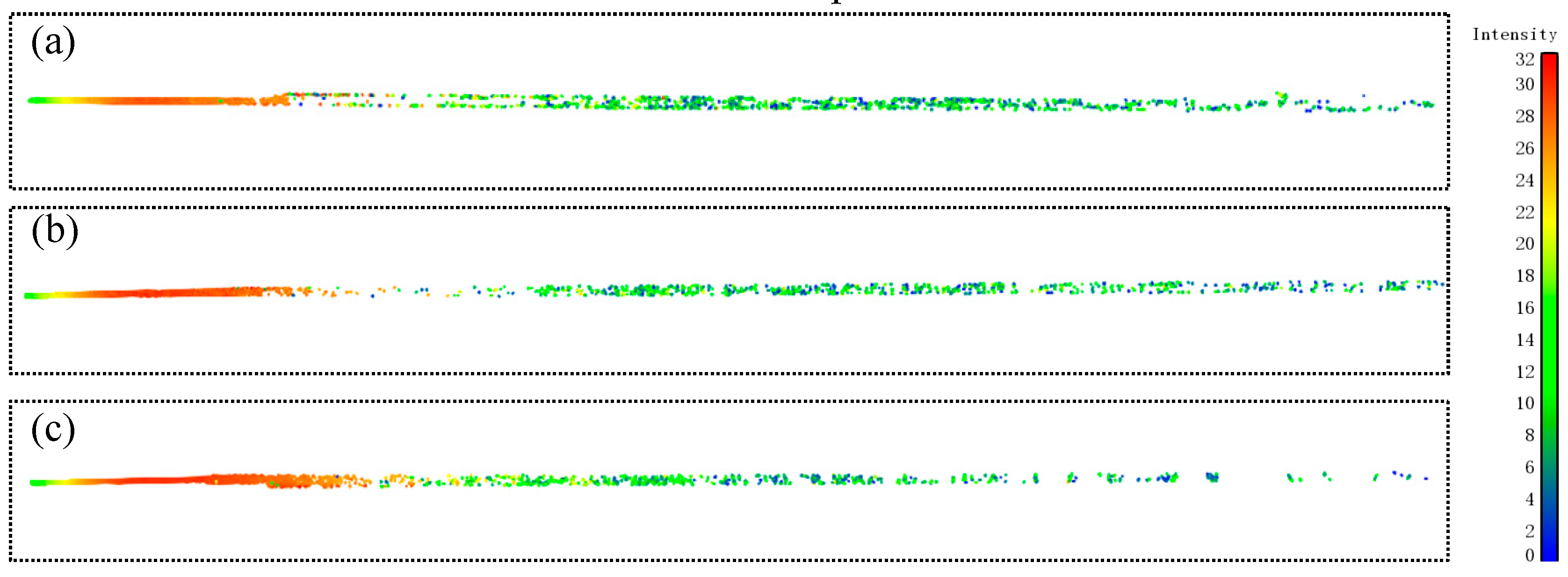
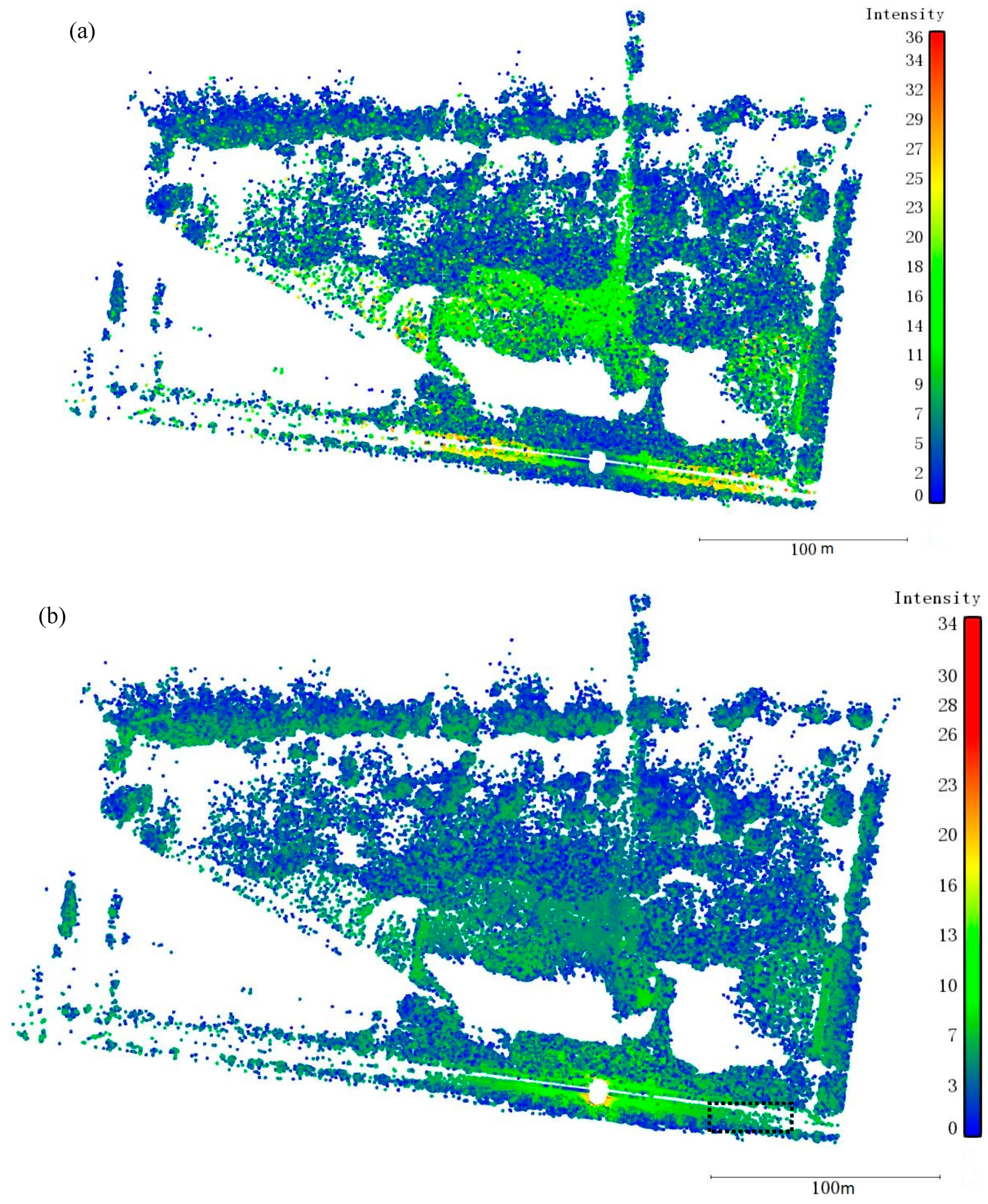
5.2. Intensity Correction

A sub-dataset of the study site (about 380 m × 250 m) was sampled. The corrected intensity data were calculated by using Equation (4) and the parameters in Table 1 and Table 2. θ s and D s were defined as 75° and 10 m, correspondingly. The point clouds of the sub-dataset colored by the original and corrected intensity data were displayed in Figure 7a,b respectively. In general, the point clouds colored by the original intensity data were visually dazzling because the original intensity data were influenced by the incidence angle and distance, making the intensity data of the same target vary significantly. Different targets using the original intensity were difficult to distinguish because the intensity data of these targets were influenced by the effects of incidence angle and distance simultaneously. The intensity data of the different targets had excessive overlaps. For example, Regions 1 and 2 belonged to the muddy flat. However, the colors (intensity) of Region 1 were completely different from that of Region 2. By contrast, Region 3 was the cement road. The colors of Region 3 were very similar to that of Region 1. This example indicated that the original intensity values of the same target may differ significantly, whereas different targets may have equal original intensity values. Therefore, it was indispensable to eliminate the effects of incidence angle and distance to obtain a corrected intensity value that can reflect the spectral characteristics of the target. After correction, a visual check and comparison with Figure 6a,b implied that different targets were easy to distinguish. In particular, the vegetation and muddy flat which corresponded to the blue and green points, respectively, became very recognizable given the corrected intensity data. Regions 1 and 2 were similar, whereas Regions 1 and 3 had completely different colors as illustrated in Figure 7b. This example indicated that the corrected intensity data directly reflected the reflectance characteristics of the scanned target. Theoretically, the surface normals of the vegetation (leaves) were difficult to reliably estimated since the vegetation faced randomly and was usually smaller than the laser footprint. This leaded to the results that the corrected intensity data of the vegetation from different parts differed slightly, as shown by the black dotted rectangle in Figure 7b.
Additionally, we derived the incidence angle-corrected and distance-corrected intensity data by using Equation (5) (Figure 8). Visually, both incidence angle-corrected and distance-corrected intensity data significantly improved the recognizability between different targets. Overall, we could roughly distinguish the contours of vegetation, road, and muddy flat based on the incidence angle-corrected and distance-corrected intensity data. However, there still existed some overlaps between different targets, e.g., a few cement road points have the same intensity values with that of the vegetation and muddy flat, as shown by the black dotted rectangles in Figure 8.
To quantitatively evaluate the intensity correction results of the improved method in the study intertidal zone, the values of C V for the intensity data were analyzed. Based on the field investigation, the main targets in the intertidal zone included three categories, i.e., vegetation, muddy flat, and cement road. To obtain the points clouds of these three categories, a semi-automatic classification was performed. First, we manually segmented and exported the points of the cement road since the points of the cement road were regularly distributed and it was very easy to identify them. Then the rest points were classified by using the “Classify Ground Points” algorithm in the commercial software LiDAR360 (Beijing GreenVally Technology Co., Ltd., Beijing, China). The algorithm can accurately classify the points into ground and non-ground points. For the rest points in the study intertidal zone, the ground and non-ground points were the muddy flat and vegetation points, respectively. The “Classify Ground Points” adopted an improved progressive triangulated irregular network (TIN) densification (IPTD) filtering algorithm that was proposed by Zhao and Guo, et al. [32]. The IPTD filtering algorithm consisted of three steps [32]: (1) acquiring potential ground seed points using the morphological method; (2) obtaining accurate ground seed points; and (3) building a TIN-based model and iteratively densifying TIN. IPTD can cope with a variety of forested landscapes, particularly both topographically and environmentally complex regions. Finally, by combining the results of manual and commercial software classifications, the points were classified into three categories (cement road, vegetation, and muddy flat) as shown by Figure 9.
The values of C V were calculated for each category before and after correction by the improved method (Table 3). After correction of the incidence angle effect, the values of C V were approximately reduced by 38%, 34%, and 23% from 0.3845, 0.3980, and 0.2458 to 0.2378, 0.2625, and 0.1882 for the muddy flat, vegetation, and cement road, respectively. By contrast, the values of C V were reduced by 26%, 18%, and 41% for these three categories after distance effect correction. After incidence angle and distance effects correction by the improved method, the values of C V were significantly decreased by 51%, 48%, and 61%. In summary, the values of C V for the intensity data of these three targets were averagely reduced by 32%, 28%, and 54% after incidence angle, distance, and incidence angle and distance effects correction.
Based on the results ( C V ) of intensity correction for the targets in the study intertidal zone, it can be concluded that both the incidence angle and distance had a crucial effect on the intensity data of long-range TLSs. Correction either of the incidence angle and distance effects can reduce the variations ( C V ) for the intensity data. The intensity correction results over the three targets proved the feasibility of the improved method and indicated that the differences in the intensity data for the different parts of the same target can be significantly reduced. The final corrected intensity data were independent of incidence angle and distance and can be used in many applications, e.g., target classification and feature extraction. In this study, the reference targets scanned in indoor environment were used to derive the incidence angle–intensity relationship. The derived relationship was then used to correct the incidence angle effect of natural targets scanned in outdoor environments. The differences of surface characteristics (e.g., roughness [26] and specular reflections [31]) between the reference targets and natural targets were ignored in this study. Considering the differences of surface characteristics could further improve the intensity correction accuracy. Additionally, if we performed measurements of the study intertidal zone from multiple scanning positions, this would enable us to directly compare the corrected intensity data for the same target from varying distances and angles. In such way, the improved method could be robustly validated. Instead, in the present study the improved method was validated from another perspective—point cloud classification based on the corrected intensity data of the study intertidal zone. The details for point cloud classifications were introduced in the following section.

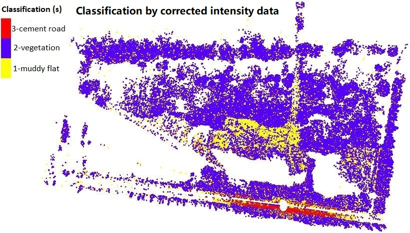
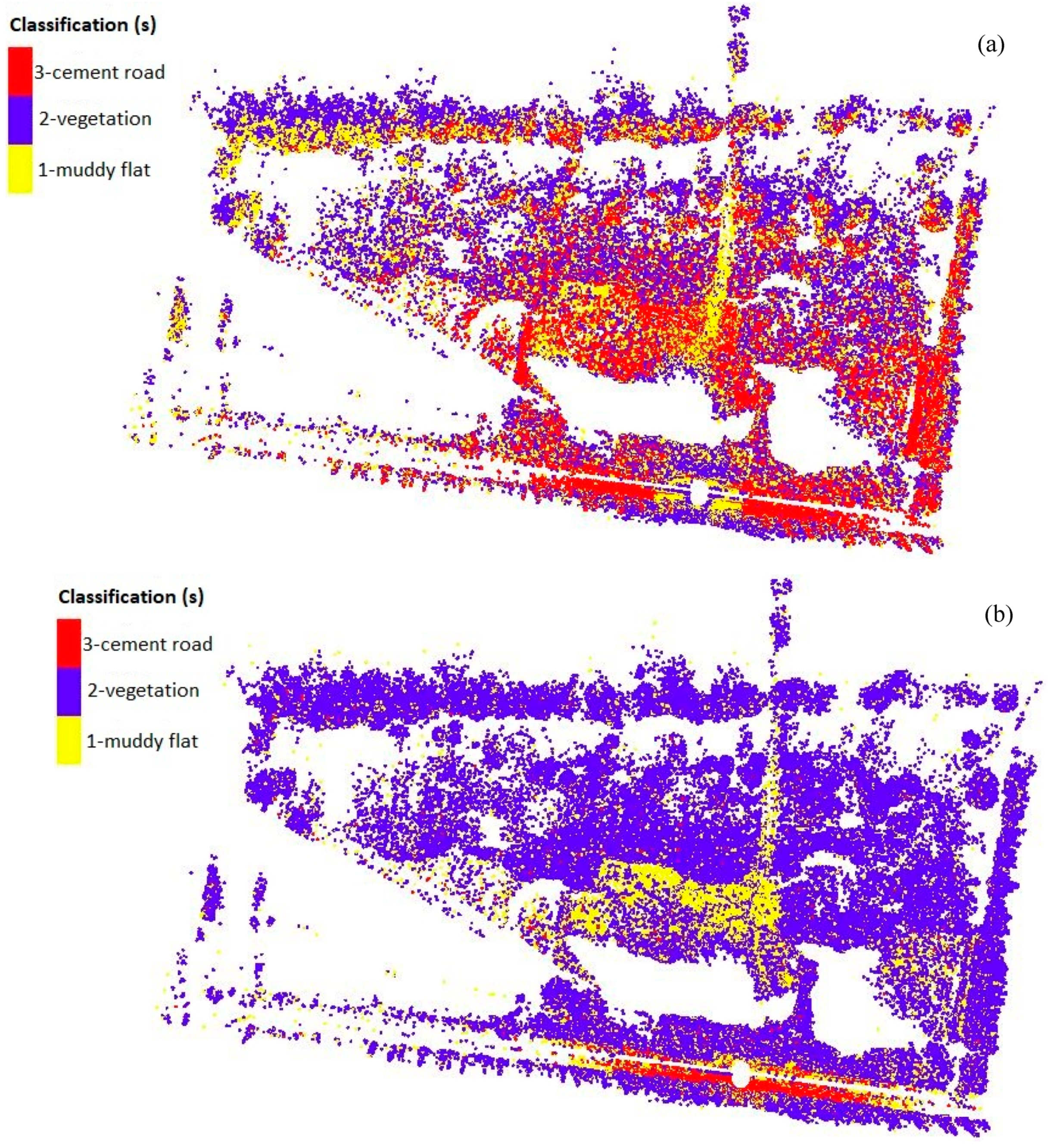
5.3. Point Cloud Classification

Point cloud classifications of the study intertidal zone were conducted by using the intensity data through k-means clustering. The classification results by the original and final corrected intensity data of the improved method were depicted in Figure 10. Generally, the classification results by the original intensity data were unsatisfactory (Figure 10a) because the original intensity data were influenced by the incidence angle and distance and cannot represent the target reflectance characteristics. Many muddy flat (yellow) and vegetation (blue) points were misclassified into cement road points (red) and some cement road points were classified into muddy flat and vegetation. On the contrary, the classification results improved significantly by using the final corrected intensity data of the improved method (Figure 10b). Only minor errors were observed in the classification results. Additionally, we classified the point cloud based on the incidence angle-corrected and distance-corrected intensity data (Figure 11). Visually, it can be seen that the incidence angle-corrected intensity data improved the vegetation classification accuracy (Figure 11a). However, many muddy flat points were still misclassified into cement road. On the contrary, the distance-corrected intensity data improved the muddy flat classification accuracy (Figure 11b). Nevertheless, massive cement road and vegetation points were classified into muddy flat.
To quantitatively evaluate the classification results in Figure 10 and Figure 11, the classification result in Figure 9 was considered true and was used as a reference. Table 4 summarized the classification results by using different intensity data. Table 5, Table 6, Table 7 and Table 8 listed the confusion matrixes for point cloud classification by using the original, incidence angle-corrected, distance-corrected, and final corrected intensity data, respectively. The F 1 scores were calculated by the producer and user accuracies in the confusion matrixes:
F 1 = 2 · P U P U
where P and U were producer and user accuracies in the confusion matrixes in Table 5, Table 6, Table 7 and Table 8, respectively. The producer accuracy P of a certain category was defined as the ratio of two numbers: the number of points that were correctly classified into this category and the actual total number of points that belonged to this category. By contrast, the user accuracy U of a certain category was defined as the ratio of the number of points that were correctly classified into this category to the total number of points that were classified into this category. The value μ in the i -th row and j -th column in the confusion matrix meant that a total number of μ points that actually belonged to the category in the j -th column were classified into the category in the i -th row. The overall accuracy was defined as the ratio of the total number of points that were correctly classified to the total number of all the points.
In comparison to the outputs of the reference classification, the overall classification accuracies were approximately 32%, 52%, 46%, and 81% for the original, incidence angle-corrected, distance-corrected, and final corrected intensity data, respectively. The classification accuracies were improved by 22%, 14%, and 49% after incidence angle, distance, and incidence angle and distance effects correction, respectively. More specifically, the F 1 scores for the vegetation and cement road were significantly improved after incidence angle effect correction (Table 6). By contrast, after distance effect correction the F 1 scores for the muddy flat and vegetation were considerably increased (Table 7). After incidence angle and distance effects correction, the producer accuracies, user accuracies, and F 1 scores for the three targets were substantially improved. The classification results of the study intertidal zone indicated that the original intensity data of long-range TLSs were significantly influenced by the incidence angle and distance. The classification results were significantly improved by the final corrected intensity data because the improved method can effectively eliminate the incidence angle and distance effects to obtain a corrected intensity that reflected the reflectance properties. The classification results further validated the feasibility of the improved method.
Compared with the algorithms that use geometrical information and need massive calculation, the classification accuracy by the intensity data of the improved method is relatively satisfactory. Moreover, classification by using geometrical information can only classify the point cloud into two categories: ground and non-ground points. As for the intertidal zone in this study, non-ground points are vegetation while ground points are muddy flat and cement road. Since the geometry between the point clouds of the muddy flat and cement road are small, point cloud classification algorithms that use geometrical information cannot classify these two categories. On the contrary, corrected intensity data are merely depend on target characteristics. Classification by the corrected intensity can accurate classify two targets whose geometrical difference are small while have different reflectance characteristics. It can be concluded that classification by corrected intensity data is easy, direct, and avoids laborious calculations.
For a better presentation of the intensity data by the improved method, three local regions of the study area were shown in Figure 12, Figure 13 and Figure 14. By comparing the RGB (Red-Green-Blue) photographs on site and corresponding regions in Figure 9 and Figure 10a,b, we concluded that the original intensity cannot reflect the actual characteristics of the target since the original intensity were influenced by the incidence angle and distance. On the contrary, the corrected intensity data by the improved method were merely related to the target reflectance characteristics and classification results based on the corrected intensity data accurately reflected the actual shape and distribution of various targets. Moreover, some features could be found by the intensity data of the improved method. For example, there were some tidal ditches as shown by the black dotted rectangle in Figure 12a. A small amount of water was existed in the ditches. The water could absorb laser and decreased the reflectance and further the corrected intensity value of the muddy flat. A decrease in the intensity made the muddy flat to be misclassified into the vegetation as shown by the black dotted rectangles in Figure 12c. Though this decreased the overall classification results by the corrected intensity data of the improved method, we could roughly distinguish and extract the shape of the ditches in Figure 12c. On the contrary, the ditches were not identifiable in Figure 12b,d. This example proved that the corrected intensity data by the improved method were related to the reflectance of the scanned target and suggested that the corrected intensity data could be further used for many applications in intertidal zones (e.g., muddy flat moisture estimation, ditches extraction).

6. Conclusions

This study proposes an improved method to correct the incidence angle and distance effects on the intensity data of long-distance TLSs. The predominant advantage of the improved method is that the distance–intensity relationship of long-distance TLSs can be accurately and detailly estimated using natural homogenous targets whereas most existing methods are unable to estimate the relationship. The results indicate that the CV of the intensity data from a homogeneous target can be reduced by approximately 54%. The classification accuracies of the case study are increased by 22%, 14%, and 49% by the incidence angle, distance, and incidence angle and distance-corrected intensity data, respectively. The classification results indicate that the improved method can accurately eliminate the variations in the original intensity data caused by the effects of incidence angle and distance and obtain a corrected intensity value that merely depends target reflectance characteristics. Theoretically, the improved method can be applied to other long-distance TLSs. However, this topic should be individually analyzed.
Since the existing methods are unable to estimate the distance–intensity relationship for long-distance TLSs, a comparison between the improved and existing methods are not conducted in this study. The instrumental configurations (e.g., instrument temperature [16]) and atmospheric conditions (e.g., humidity, pressure) are ignored in the study. Considering these effects would further improve the intensity correction accuracy. Moreover, the incidence angle effect mainly depends on the target surface characteristics [10,37]. In this study, the incidence angle–intensity relationship derived from reference targets is used to correct the incidence angle effect of natural targets. The differences of surface characteristics are ignored. Target surface characteristics, such as roughness [19,26,39] and specular reflections [31], should be considered in correcting the incidence angle effect to further improve the intensity correction accuracy.

Author Contributions

All the authors of the present work contributed to the results and discussion of the results. K.T. proposed the method and derived the formulas; K.T., J.C. and W.Q. conceived, designed, and performed the experiments; K.T. and F.S. analyzed the data; W.Z. and F.S. contributed materials and analysis tools; and K.T. and X.C. wrote the paper.

Funding

This research was funded by the Shanghai Sailing Program, grant number 18YF1406800, China Postdoctoral Science Foundation, grant number 2017M620141, State Key Laboratory of Estuarine and Coastal Research (East China Normal University), grant number 2017RCDW06, and National Natural Science Foundation of China, grant number 41671449.

Acknowledgments

The authors are very grateful to Xuelin Zhang from Beijing GreenVally Technology Co., Ltd., China, for providing trial permission of the software LiDAR360.

Conflicts of Interest

The authors declare no conflict of interest.

References

  1. Telling, J.; Lyda, A.; Hartzell, P.; Glennie, C. Review of Earth science research using terrestrial laser scanning. Earth Sci. Rev. 2017, 169, 35–68. [Google Scholar] [CrossRef] [Green Version]
  2. Wang, W.; Zhao, W.; Huang, L.; Vimarlund, V.; Wang, Z. Applications of terrestrial laser scanning for tunnels: A review. J. Traff. Trans. Eng. 2014, 1, 325–337. [Google Scholar] [CrossRef]
  3. Dassot, M.; Constant, T.; Fournier, M. The use of terrestrial LiDAR technology in forest science: Application fields, benefits and challenges. Ann. For. Sci. 2011, 68, 959–974. [Google Scholar] [CrossRef]
  4. Liang, X.; Kankare, V.; Hyyppä, J.; Wang, Y.; Kukko, A.; Haggrén, H.; Yu, X.; Kaartinen, H.; Jaakkola, A.; Guan, F.; et al. Terrestrial laser scanning in forest inventories. ISPRS J. Photogramm. Remote Sens. 2016, 115, 63–77. [Google Scholar] [CrossRef] [Green Version]
  5. Pinkerton, H.; Applegarth, L.J.; James, M.R. Detecting the development of active lava flow fields with a very-long-range terrestrial laser scanner and thermal imagery. Geophys. Res. Lett. 2009, 36, 355. [Google Scholar]
  6. López-Moreno, J.I.; Revuelto, J.; González, E.A.; Sanmiguel-Vallelado, A.; Fassnacht, S.R.; Deems, J.; Morán-Tejeda, E. Using very long-range terrestrial laser scanner to analyze the temporal consistency of the snowpack distribution in a high mountain environment. J. Mt. Sci. 2017, 14, 823–842. [Google Scholar] [CrossRef]
  7. Xie, W.; He, Q.; Zhang, K.; Guo, L.; Wang, X.; Shen, J.; Cui, Z. Application of terrestrial laser scanner on tidal flat morphology at a typhoon event timescale. Geomorphology 2017, 292, 47–58. [Google Scholar] [CrossRef]
  8. Thers, H.; Brunbjerg, A.K.; Læssøe, T.; Ejrnæs, R.; Bøcher, P.K.; Svenning, J.-C. Lidar-derived variables as a proxy for fungal species richness and composition in temperate Northern Europe. Remote Sens. Environ. 2017, 200, 102–113. [Google Scholar] [CrossRef]
  9. Kaasalainen, S.; Krooks, A.; Kukko, A.; Kaartinen, H. Radiometric Calibration of Terrestrial Laser Scanners with External Reference Targets. Remote Sens. 2009, 1, 144–158. [Google Scholar] [CrossRef] [Green Version]
  10. Kaasalainen, S.; Jaakkola, A.; Kaasalainen, M.; Krooks, A.; Kukko, A. Analysis of Incidence Angle and Distance Effects on Terrestrial Laser Scanner Intensity: Search for Correction Methods. Remote Sens. 2011, 3, 2207–2221. [Google Scholar] [CrossRef] [Green Version]
  11. Höfle, B.; Pfeifer, N. Correction of laser scanning intensity data: Data and model-driven approaches. ISPRS J. Photogramm. Remote Sens. 2007, 62, 415–433. [Google Scholar] [CrossRef]
  12. Armesto-González, J.; Riveiro-Rodríguez, B.; González-Aguilera, D.; Rivas-Brea, M.T. Terrestrial laser scanning intensity data applied to damage detection for historical buildings. J. Archaeol. Sci. 2010, 37, 3037–3047. [Google Scholar] [CrossRef]
  13. Yan, W.Y.; Shaker, A. Radiometric normalization of overlapping LiDAR intensity data for reduction of striping noise. Int. J. Digit. Earth 2015, 9, 1–13. [Google Scholar]
  14. Poux, F.; Neuville, R.; Van Wersch, L.; Nys, G.-A.; Billen, R. 3D Point Clouds in Archaeology: Advances in Acquisition, Processing and Knowledge Integration Applied to Quasi-Planar Objects. Geosciences 2017, 7, 96. [Google Scholar] [CrossRef]
  15. Yan, W.Y.; Shaker, A. Radiometric Correction and Normalization of Airborne LiDAR Intensity Data for Improving Land-Cover Classification. IEEE Trans. Geosci. Remote Sens. 2014, 52, 7658–7673. [Google Scholar]
  16. Errington, A.F.C.; Daku, B.L.F. Temperature Compensation for Radiometric Correction of Terrestrial LiDAR Intensity Data. Remote Sens. 2017, 9, 356. [Google Scholar] [CrossRef]
  17. Zhu, X.; Wang, T.; Darvishzadeh, R.; Skidmore, A.K.; Niemann, K.O. 3D leaf water content mapping using terrestrial laser scanner backscatter intensity with radiometric correction. ISPRS J. Photogramm. Remote Sens. 2015, 110, 14–23. [Google Scholar] [CrossRef]
  18. Tan, K.; Cheng, X. Correction of Incidence Angle and Distance Effects on TLS Intensity Data Based on Reference Targets. Remote Sens. 2016, 8, 251. [Google Scholar] [CrossRef]
  19. Xu, T.; Xu, L.; Yang, B.; Li, X.; Yao, J. Terrestrial Laser Scanning Intensity Correction by Piecewise Fitting and Overlap-Driven Adjustment. Remote Sens. 2017, 9, 1090. [Google Scholar] [CrossRef]
  20. Fang, W.; Huang, X.; Zhang, F.; Li, D. Intensity Correction of Terrestrial Laser Scanning Data by Estimating Laser Transmission Function. IEEE Trans. Geosci. Remote Sens. 2015, 53, 942–951. [Google Scholar] [CrossRef]
  21. Franceschi, M.; Teza, G.; Preto, N.; Pesci, A.; Galgaro, A.; Girardi, S. Discrimination between marls and limestones using intensity data from terrestrial laser scanner. ISPRS J. Photogramm. Remote Sens. 2009, 64, 522–528. [Google Scholar] [CrossRef]
  22. Teo, T.-A.; Yu, H.-L. Empirical Radiometric Normalization of Road Points from Terrestrial Mobile Lidar System. Remote Sens. 2015, 7, 6336–6357. [Google Scholar] [CrossRef] [Green Version]
  23. Höfle, B. Radiometric Correction of Terrestrial LiDAR Point Cloud Data for Individual Maize Plant Detection. IEEE Geosci. Remote Sens. Lett. 2014, 11, 94–98. [Google Scholar] [CrossRef]
  24. Burton, D.; Dunlap, D.B.; Wood, L.J.; Flaig, P.P. LiDAR intensity as a remote sensor of rock properties. J. Sediment. Res. 2011, 81, 339–347. [Google Scholar] [CrossRef]
  25. Tan, K.; Cheng, X. Intensity data correction based on incidence angle and distance for terrestrial laser scanner. J. Appl. Remote Sens. 2015, 9, 94094. [Google Scholar] [CrossRef]
  26. Carrea, D.; Abellan, A.; Humair, F.; Matasci, B.; Derron, M.-H.; Jaboyedoff, M. Correction of terrestrial LiDAR intensity channel using Oren–Nayar reflectance model: An application to lithological differentiation. ISPRS J. Photogramm. Remote Sens. 2016, 113, 17–29. [Google Scholar] [CrossRef]
  27. Kashani, A.G.; Olsen, M.J.; Parrish, C.E.; Wilson, N. A Review of LiDAR radiometric processing: From Ad Hoc intensity correction to rigorous radiometric calibration. Sensors 2015, 15, 28099–28128. [Google Scholar] [CrossRef]
  28. Soudarissanane, S.; Lindenbergh, R.; Menenti, M.; Teunissen, P. Scanning geometry: Influencing factor on the quality of terrestrial laser scanning points. ISPRS J. Photogramm. Remote Sens. 2011, 66, 389–399. [Google Scholar] [CrossRef]
  29. Herrero-Pascual, J.; Felipe-García, B.; Hernández-López, D.; Rodríguez-Gonzálvez, P.; González-Aguilera, D.; Del Pozo, S. Multispectral Radiometric Analysis of Façades to Detect Pathologies from Active and Passive Remote Sensing. Remote Sens. 2016, 8, 80. [Google Scholar] [CrossRef]
  30. Tan, K.; Cheng, X.; Ding, X.; Zhang, Q. Intensity Data Correction for the Distance Effect in Terrestrial Laser Scanners. IEEE J. Sel. Top. Appl. Earth Obs. Remote Sens. 2016, 9, 304–312. [Google Scholar] [CrossRef]
  31. Tan, K.; Cheng, X. Specular Reflection Effects Elimination in Terrestrial Laser Scanning Intensity Data Using Phong Model. Remote Sens. 2017, 9, 853. [Google Scholar] [CrossRef]
  32. Zhao, X.; Guo, Q.; Su, Y.; Xue, B. Improved progressive TIN densification filtering algorithm for airborne LiDAR data in forested areas. ISPRS J. Photogramm. Remote Sens. 2016, 117, 79–91. [Google Scholar] [CrossRef] [Green Version]
  33. Pesci, A.; Teza, G.; Ventura, G. Remote sensing of volcanic terrains by terrestrial laser scanner: Preliminary reflectance and RGB implications for studying Vesuvius crater (Italy). Ann. Geophys. 2008, 51, 633–653. [Google Scholar]
  34. Prantl, H.; Nicholson, L.; Sailer, R.; Hanzer, F.; Juen, I.F.; Rastner, P. Glacier Snowline Determination from Terrestrial Laser Scanning Intensity Data. Geosciences 2017, 7, 60. [Google Scholar] [CrossRef]
  35. Podgórski, J.; Pętlicki, M.; Kinnard, C. Revealing recent calving activity of a tidewater glacier with terrestrial LiDAR reflection intensity. Cold Regions Sci. Technol. 2018, 151, 288–301. [Google Scholar] [CrossRef]
  36. Olsoy, P.J.; Glenn, N.F.; Clark, P.E. Estimating Sagebrush Biomass Using Terrestrial Laser Scanning. Rangel. Ecol. Manag. 2014, 67, 224–228. [Google Scholar] [CrossRef]
  37. Kukko, A.; Kaasalainen, S.; Litkey, P. Effect of incidence angle on laser scanner intensity and surface data. Appl. Opt. 2008, 47, 986–999. [Google Scholar] [CrossRef]
  38. Kaasalainen, S.; Vain, A.; Krooks, A.; Kukko, A. Topographic and distance effects in laser scanner intensity correction. Int. Arch. Photogramm. Remote Sens. Spat. Inf. Sci. 2009, 38, 219–222. [Google Scholar]
  39. Cheng, X.; Tan, K.; Cheng, X. Modeling hemispherical reflectance for natural surfaces based on terrestrial laser scanning backscattered intensity data. Opt. Express 2016, 24, 22971. [Google Scholar]
  40. Ding, Q.; Chen, W.; King, B.; Liu, Y.; Liu, G. Combination of overlap-driven adjustment and Phong model for LiDAR intensity correction. ISPRS J. Photogramm. Remote Sens. 2013, 75, 40–47. [Google Scholar] [CrossRef]
  41. Poullain, E.; Garestier, F.; Levoy, F.; Bretel, P. Analysis of ALS Intensity Behavior as a Function of the Incidence Angle in Coastal Environments. IEEE J. Sel. Top. Appl. Earth Obs. Remote Sens. 2016, 9, 1–13. [Google Scholar] [CrossRef]
  42. Riegl_VZ-4000_Datasheet. Available online: http://www.riegl.com/uploads/tx_pxpriegldownloads/RIEGL_VZ-4000_Datasheet_2018-12-05.pdf (accessed on 1 January 2019).
  43. RiSCAN PRO 2.0. Available online: http://www.riegl.com/products/software-packages/riscan-pro/ (accessed on 6 December 2018).
  44. Jueterbock, A.; Smolina, I.; Coyer, J.A.; Hoarau, G. The fate of the Arctic seaweedFucus distichusunder climate change: an ecological niche modeling approach. Ecol. Evol. 2016, 6, 1712–1724. [Google Scholar] [CrossRef] [PubMed] [Green Version]
  45. Hemery, L.G.; Marion, S.R.; Romsos, C.G.; Kurapov, A.L.; Henkel, S.K. Ecological niche and species distribution modelling of sea stars along the Pacific Northwest continental shelf. Divers. Distrib. 2016, 22, 1314–1327. [Google Scholar] [CrossRef]
  46. Cuadrado, D.G.; Perillo, G.M.; Vitale, A.J. Modern microbial mats in siliciclastic tidal flats: Evolution, structure and the role of hydrodynamics. Mar. Geol. 2014, 352, 367–380. [Google Scholar] [CrossRef]
  47. Guo, C.; He, Q.; Van Prooijen, B.C.; Guo, L.; Manning, A.J.; Bass, S. Investigation of flocculation dynamics under changing hydrodynamic forcing on an intertidal mudflat. Mar. Geol. 2018, 395, 120–132. [Google Scholar] [CrossRef]
  48. Fabbri, S.; Giambastiani, B.M.; Sistilli, F.; Scarelli, F.; Gabbianelli, G. Geomorphological analysis and classification of foredune ridges based on Terrestrial Laser Scanning (TLS) technology. Geomorphology 2017, 295, 436–451. [Google Scholar] [CrossRef]
Figure 1. Flowchart of the improved method.
Remotesensing 11 00331 g001
Figure 2. Diagram for the setup of the laboratory experiments.
Remotesensing 11 00331 g002
Figure 3. Point cloud for the narrow (about 0.5 m) sampled slices of the cement road with distances from 5 m to 500 m colored by the original intensity data. (a) Site 1 (31°46′03″N, 121°11′01″E). (b) Site 2 (31°46′13″N, 121°11′15″E). (c) Site 3 (31°49′24″N, 121°12′43″E). The number of points is 103,970, 116,242, and 135,561 for Sites 1, 2, and 3, respectively.
Remotesensing 11 00331 g003
Figure 4. (a) Experimental results between the incidence angle and original intensity of the four reference targets. The black lines are the 3rd-degree fitting polynomials. (b) Incidence angle with respect to the corrected intensity data of the four reference targets by the first equation of Equation (5) ( θ s = 0°).
Remotesensing 11 00331 g004
Figure 5. (ac): Original intensity data. (df): Incidence angle-corrected intensity data and 7th-degree fitting polynomials. (gi): Final corrected intensity data by the improved method. (a,d,g): Cement road from Sites 1. (b,e,h): Cement road from Sites 2. (c), (f), and (i): Cement road from Sites 3. θ s and d s are defined as 75° and 10 m, correspondingly. The vertical and horizontal axes for all the figures are intensity and distance, respectively. The number of points is 103,970, 116,242, and 135,561 for Sites 1, 2, and 3, respectively.
Remotesensing 11 00331 g005
Figure 6. (a) Panoramic image of the study site captured by a camera. (b) Orthophoto of the study site provided by United States Geological Survey (USGS, https://earthexplorer.usgs.gov/). (c) Point clouds of the study site colored by original intensity data in RiSCAN PRO v1.8.1.
Remotesensing 11 00331 g006
Figure 7. Point cloud colored by intensity. (a) Original intensity data. (b) Final corrected intensity by the improved method. The total number of points is 931,381. The white parts among the figures have no measured points considering water accumulation or occlusion.
Remotesensing 11 00331 g007
Figure 8. Point cloud colored by intensity. (a) Incidence angle-corrected intensity by using the first equation of Equation (5). (b) Distance-corrected intensity by using the second equation of Equation (5). The total number of points is 931,381. The white parts among the figures have no measured points considering water accumulation or occlusion.
Remotesensing 11 00331 g008
Figure 9. Combination of manual and commercial software classification (“Classify Ground Points” algorithm which use the geometrical information of the point cloud in LiDAR360).
Remotesensing 11 00331 g009
Figure 10. Classification results according to the intensity data using k-means clustering. (a) Original intensity data. (b) Final corrected intensity data by the improved method.
Remotesensing 11 00331 g010
Figure 11. Classification results according to the intensity data of the improved method using k-means clustering. (a) Incidence angle-corrected intensity data. (b) Distance-corrected intensity data.
Remotesensing 11 00331 g011
Figure 12. Comparison of (a) an RGB photograph on site and the corresponding region in the classification results by (b) original intensity data, (c) corrected intensity data by the improved method, and (d) manual and software (LiDAR360) combination. The yellow, blue, and red points represent muddy flat, vegetation and cement road, respectively. Ditches are in the black dotted rectangles.
Remotesensing 11 00331 g012
Figure 13. Comparison of (a) an RGB photograph on site and the corresponding region in the classification results by (b) original intensity data, (c) corrected intensity data by the improved method, and (d) manual and software (LiDAR360) combination. The yellow, blue, and red points represent muddy flat, vegetation and cement road, respectively.
Remotesensing 11 00331 g013
Figure 14. Comparison of (a) an RGB photograph on site and the corresponding region in the classification results by (b) original intensity data, (c) corrected intensity data by the improved method, and (d) manual and software (LiDAR360) combination. The yellow, blue, and red points represent muddy flat, vegetation and cement road, respectively.
Remotesensing 11 00331 g014
Table 1. Mean values of the polynomial parameters for f2(θ).
N 2 α 0 α 1 α 2 α 3
31−3.38 × 10−32.38 × 10−5−9.73 × 10⁻⁷
Table 2. Mean values of the polynomial parameters for f3(d).
N 3 β 0 β 1 β 2 β 3 β 4 β 5 β 6 β 7
7−7.49 × 10−22.5527.55140.07−377.53552.08−394.381
Table 3. Values of CV for the intensity data before and after correction.
Data SourceMuddy FlatVegetationCement Road
Original intensity0.38450.39800.2458
Incidence angle-corrected intensity0.23780.26250.1882
Distance-corrected intensity0.28450.32670.1442
Final corrected intensity0.18960.20550.0894
Table 4. Point cloud classification results by different data sources.
Data SourceMuddy FlatVegetationCement Road
Original intensityNumber: 181,183
Intensity: 14–22
Number: 131,140
Intensity: 0–14
Number: 619,058
Intensity: 22–32
Incidence angle-corrected intensityNumber: 472,214
Intensity: 6–13
Number: 262,525
Intensity: 0–6
Number: 196,642
Intensity: 13–36
Distance-corrected intensityNumber: 307,959
Intensity: 4–8
Number: 569,008
Intensity: 0–4
Number: 54,414
Intensity: 8–34
Final corrected intensityNumber: 358,925
Intensity: 4–7
Number: 366,145
Intensity: 0–4
Number: 206,311
Intensity: 7–33
Manual and commercial software classificationNumber: 285,073Number: 453,347Number: 192,961
Table 5. Confusion matrix of classification by original intensity data.
Muddy FlatVegetationCement RoadTotalUser Acuracy (U)
Muddy flat102,83553,11425,234181,18356.76%
Vegetation24,40866,38940,343131,14050.62%
Cement road157,830333,844127,384619,05820.58%
Total285,073453,347192,961931,381
Producer accuracy ( P ).36.07%14.64%66.05%
F 1 44.11%22.%31.38% Overall accuracy: 31.85%
Table 6. Confusion matrix of classification by incidence angle-corrected intensity data.
Muddy FlatVegetationCement RoadTotalUser Accuracy (U)
Muddy flat173,437249,67449,103472,21436.73%
Vegetation50,761190,26421,500262,52572.47%
Cement road60,87513,409122,358196,64262.22%
Total285,073453,347192,961931,381
Producer accuracy ( P )60.84%41.97%63.41%
F 1 45.81%53.16%62.81% Overall accuracy: 52.19%
Table 7. Confusion matrix of classification by distance-corrected intensity data.
Muddy FlatVegetationCement RoadTotalUser Accuracy (U)
Muddy flat221,322281,08766,599569,00838.90%
Vegetation61,361164,58182,017307,95953.44%
Cement road2,3907,67944,34554,41481.50%
Total285,073453,347192,961931,381
Producer accuracy ( P )77.64%36.30%22.98%
F 1 51.83%43.23%35.85% Overall accuracy: 46.19%
Table 8. Confusion matrix of classification by final corrected intensity data.
Muddy FlatVegetationCement RoadTotalUser Accuracy (U)
Muddy flat244,065104,50810,352358,92568.00%
Vegetation38,342325,5402,263366,14588.91%
Cement road2,66623,299180,346206,31187.41%
Total285,073453,347192,961931,381
Producer accuracy ( P )85.61%71.81%93.46%
F 1 75.80%79.45%90.33% Overall accuracy: 80.52%

