Variability of the Great Whirl and Its Impacts on Atmospheric Processes

Abstract

Using satellite remote sensing data and re-analysis products for the period of 1993–2015, the variation of a large anticyclonic eddy, the so-called Great Whirl (GW), located in the Northwest Indian Ocean off the coast of Somali, and its impacts on atmosphere were investigated. The GW is generated in early summer and decays in late fall every year. The center of the GW is located at 7.73°N, 53.20°E. The mean lifetime, sea level anomaly (SLA) difference, sea surface temperature anomaly (SSTA), radius, normalized vorticity, eddy kinetic energy (EKE), and deformation rate are 169 days, 0.07 m, 0.83 °C, 116.86 km, −0.53, 0.08 ${\mathrm{m}}^2·{\mathrm{s}}^{-2}$, and 0.58, respectively. All these variables exhibit interannual variations. Composite analyses show that the maximum values of sea surface temperature (SST), wind, and water vapor anomalies occur in the northwest of the GW center. The fitting coefficient between the SST and wind speed anomaly is 1.1, indicating that, corresponding to 1 °C increases of the SST, the wind speed increases by about 1.1 $\mathrm{m}·{\mathrm{s}}^{-1}$, and the fitting coefficient between the SST and water vapor anomaly is 0.45, indicating that water vapor increases by about 0.45 mm in response to 1 °C increases in the SST. In the vertical direction, the maximum and minimum values of vertical velocity anomalies and vertical transport of transient zonal momentum occur over the GW at about 900 hPa, and wind speed anomalies occur at about 950 hPa. Both the positive transport anomalies of transient zonal momentum and the positive vertical velocity anomalies on the west side of the GW can accelerate the wind speed in the lower level.

1. Introduction

The Arabian Sea, located in the northwestern Indian Ocean, is dominated by the monsoon system, with large seasonal reversals of winds [1]. Under the influence of the monsoon, the Somali Current is the only western boundary flow in the world ocean that displays seasonal change in current direction [2]. In winter, the Somali warm current flows from north to south, but in summer, the cold water due to the upwelling along the coast of Somalia flows from south to north. In this seasonal varying environment, a large anticyclonic eddy, so-called Great Whirl (GW), is generated in the early summer, evolves in the following months, and decays in the early winter every year [3]. It is a large, persistent anticyclonic eddy with a warm sea surface temperature (SST) observed at a quasi-steady location in the Arabian Sea during a period spanning half a year.

The GW was reported first by Bruce et al. [4,5], who analyzed the observed data and found the presence of the GW every year in the north of the Somali Current. After the onset of the southwest monsoon along the coast of Somalia occurs in late May, a weak coastal current forms and flows across the equator from south to north. At the same time, the Somali Current begins to form, driven by the coastal winds, and keeps moving northward [6]. When the Somali Current flows northward and stays between 5°N and 10°N, a mesoscale clockwise rotating flow, the Great Whirl, is generated [1,4]. During August and September, the southwest monsoon intensity increases, and the GW enters a mature period. During October and November, the southwest monsoon gradually weakens, resulting in the decay of the GW.

A few generation mechanisms for the GW are proposed in literature: Rossby wave, the Somali coastline tilting, and barotropic instability are considered to be possible factors contributing to the generation of the GW [6,7,8,9]. Beal et al. [6,7] analyzed satellite altimeter data and suggested that the Rossby wave plays an important role in the generation of the GW. Vic et al. [10] applied a numerical model to further confirm the role of cross-basin propagating Rossby waves in the GW generation. McCreary and Kundu [8] suggested that the sloping coastline of Somali is the main cause of the formation of the GW, and can prevent the GW from moving northward. Jensen [9] suggested that barotropic instability is probably the cause of the generation of the GW by using a four-layer model.

The center of the GW can be determined from satellite altimeter data. The mean position of the GW center is about 8°N and 53°E, and the mean lifetime is about 166 days, with interannual variation [6,7,11]. Results from Cao et al. [11] show that the center of the GW shifted westward in 1993, 1999, and 2003, shifted eastward in 1995 and 2005, shifted southward in 1999, 2003, and 2007, and shifted northward in 1995, 1997, and 2005.

The variation of the GW center position is suggested to be caused by either wind or oceanic processes [12,13,14]. Luther et al. [12] used a nonlinear reduced gravity model to simulate the influence of Socotra Island (Socotra Gyre) on the northward propagation of the GW. The presence of Socotra Island limits the GW to the south of the island; if Socotra Island did not exist, the GW could continue to progress northwards. Luther et al. [12] suggested that the interannual variation characteristics of the GW are almost completely independent of the characteristics of the interior of the ocean, and are determined only by the interannual variation of wind stress. Subsequently, Luther et al. [13] used 23 years (1954–1976) of observed wind data as a forcing field to study the interannual variation characteristics of the GW, and found that the GW moves northward following the line of zero wind stress curl marking the core of the Findlater jet. Wirth et al. [14] studied the interannual variation of the meridional position of the GW center based on a 1/3° × 1/3°primary equation model and a 1/9° × 1/9° reduced gravity model. Their results demonstrate that the main reason for the interannual variation of the meridional position of the GW center is oceanic instability, rather than changes in sea surface wind field. Therefore, there is no conclusion for the reason causing the interannual variation of the GW.

The presence of the GW with the warm SST can influence the physical processes. The mesoscale air-sea interaction has been extensively studied in the northwestern Indian Ocean and other regions. Using satellite and in situ observational data, Vecchi et al. [15] confirmed that the western Arabian Sea exhibits strong air–sea coupling during the southwest monsoon. Their results show that weak (strong) wind velocities overlie cold (warm) SST, which is the same as Nonaka’s result [16]. Mafimbo et al. [17] indicated that high covariability in mesoscale winds and SSTs are found over the upwelling region along the Somali coast. Chelton et al. [18] indicated that the change of surface winds blowing across SST fronts can result in most of the small-scale variability in the divergence filed, and the resulting convergences and divergences generate vertical motion that can influence atmospheric dynamics and thermodynamics at higher levels in the atmosphere. Koseki et al. [19] used a high-resolution atmospheric circulation model to study the response characteristics of the atmospheric boundary layer to mesoscale ocean eddies in the Kuroshio extension. They showed that the spatial patterns of surface wind anomalies and mesoscale SST anomalies are significantly correlated. Frenger et al. [20] examined the relationship between eddies in the Southern Ocean and the atmosphere. Their results quantitatively show that anticyclonic and cyclonic eddies cause positive and negative anomalies of near-surface wind speed, cloud fraction, and rain rate, respectively. Ma et al. [21] analyzed the composition of more than 35,000 marine eddies in the Kuroshio extension area from 2006 to 2009, and found that the cold (warm) vortices cause the sea surface wind speed to decrease (increase) and reduce (enhance) the latent heat flux, sensible heat flux, cloud liquid water, and precipitation rate. Ma et al. [22] used high-resolution satellite observations to reveal distinct seasonal variations in atmospheric responses to oceanic eddies in the Kuroshio Extension region, characterized by much stronger surface wind speed and heat flux responses in the cold seasons (winter and spring) than in the warm seasons (summer and autumn). According to our knowledge, there are few reports in literature studying atmospheric response to the GW. Seo et al. [23] indicated that the climatological wind speed maximum of the Somali Jet is co-located with the GW, and that there can be a potential feedback on the structure of the low-level winds by using a coupled model named the Scripps Coupled Ocean–Atmospheric Regional model. Seo [24] used the same model to show that the mesoscale SST–wind interaction can influence the wind and Ekman pumping over the GW. When the effect of the SST–wind interaction is suppressed, the enhanced wind and the weakened Ekman pumping dipole cause the GW to extend northeastward, delaying the Somali Current separation by 1°.

Based on the above reviews, we can see that previous research has investigated numerous aspects of the GW, however, further studies are needed to clarify its variations and address its impacts on atmospheric processes and other related issues. In the present study, we applied satellite remote sensing data of both atmospheric and oceanic variables to examine the variation of the GW and its influences on the atmospheric boundary layer. The study area was 0°–30°N, 40°–80°E, which fully covers the area of the GW. The remainder of this paper is organized as follows: datasets and methods used are introduced in Section 2. Mean state and interannual variations of the GW and atmospheric response to the GW are discussed in Section 3. Summary and discussion are presented in Section 4.

2. Data and Methods

2.1. Data

This study employed satellite remote sensing data (sea level anomalies (SLA), SST) [25,26,27], Tropical Rainfall Measuring Mission (TRMM) microwave imager (TMI) data [28], and ERA-Interim reanalysis (interim ECMWF Re-Analysis) data [29]. The details of these data are described below.

2.1.1. Satellite Altimeter Measured SLA Data

The SLA and SLA-derived geostrophic currents data employed in the present study were downloaded from the AVISO (Archiving, Validation, and Interpretation of Satellite Oceanographic Data). The 23 year (January 1993–December 2015) spatial and temporal resolution is 0.25$°$ × 0.25$°$ and daily, respectively. Both of these datasets were used to explore some features of GW.

2.1.2. Satellite Remote Sensing SST Data

The AVHRR (advanced very high resolution radiometer) SST data with 0.25$°$ × 0.25$°$ spatial resolution and daily sampling were used in this study. AVHRR is a sensor carried on the NOAA (National Oceanic and Atmospheric Administration) series of meteorological satellites. Since the launch of the TIROS-N satellite in 1979, the AVHRR sensor has continued to perform ground observation missions. The same period of SST data as that of the SLA data was used.

2.1.3. TMI Data

The TRMM satellite was launched on 27 November 1997 and provided data until 8 April 2015. It was the first meteorological satellite dedicated to the quantitative measurement of tropical and subtropical precipitation. The observation range was between 40 degrees north and south latitude. Sea surface temperature measured by TRMM microwave imager (TMI) reduces the influence of clouds, therefore, it is more accurate and reliable. This study selected TMI sea surface temperature, wind speed, and water vapor data with 0.25$°$ × 0.25$°$ spatial resolution from 1998 to 2014 to analyze the impacts of the GW on the atmosphere at the sea surface.

2.1.4. ERA-Interim Reanalysis Data

The ERA-Interim reanalysis data were used in the present study. Multiple variables (zonal wind velocity, meridional wind velocity, and vertical wind speed) with 11 layers (from 1000 hPa to 500 hPa with 50 hPa interval) and 0.25$°$ × 0.25$°$ spatial resolution from 1998 to 2014 were used to analyze the impacts of the GW on the atmosphere in the vertical direction.

2.2. Methods

2.2.1. Eddy Automatic Detection.

The eddy detection method used in this paper was proposed by Nencioli [30]. Four constraints were derived in conformance with the eddy velocity field definition and characteristics described below. Eddy centers were determined at the points where all of the constraints were satisfied. The four constraints follow:

(1) along an east–west (EW) section, v reverses sign across the eddy center and its magnitude increases away from it;

(2) along a north–south (NS) section, u reverses sign across the eddy center and its magnitude increases away from it: the sense of rotation has to be the same as for v;

(3) velocity magnitude is a local minimum at the eddy center;

(4) around the eddy center, the directions of the velocity vectors have to change with a constant sense of rotation, and the directions of two neighboring velocity vectors have to lay within the same or two adjacent quadrants (the four quadrants are defined by the north–south and west–east axes: the first quadrant encompasses all the directions from east to north, the second quadrant encompasses the directions from north to west, the third quadrant encompasses the directions from west to south, and the fourth quadrant encompasses the directions from south to east.

The constraints require two parameters to be specified: one for the first, second, and fourth constraints, and one for the third one. The first parameter, a, defines how many grid points away the increases in magnitude of v along the EW axes and u along the NS axes are checked. It also defines the curve around the eddy center, along which the change in direction of the velocity vectors is inspected. The second parameter, b, defines the dimension (in grid points) of the area used to define the local minimum of velocity. These two parameters give flexibility to the algorithm: they set the minimum size of the detectable vortices and allow the algorithm to be applied to grids with different resolutions. The value of these two parameters has a significant effect on the results of the eddy detection.

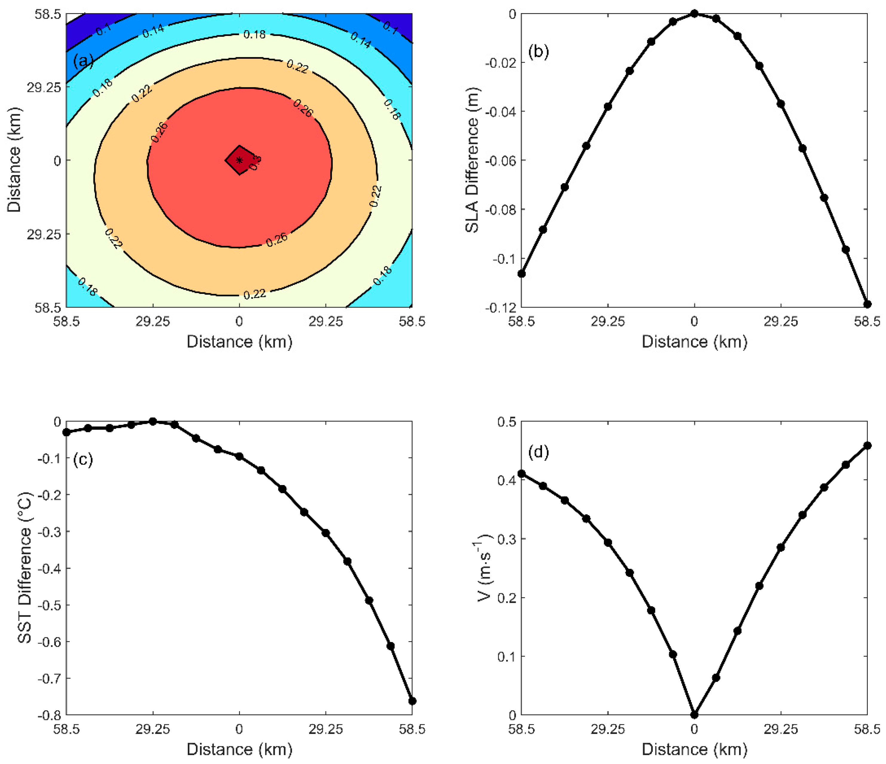
2.2.2. Composite Analysis

For composite analyses, we collocated atmospheric and oceanic variables within a box area of 4° latitude by 4° longitude centered about the GW center. To obtain the small-scale characteristics of variables of interest, we removed a zonal 8° moving average from the original data.

2.2.3. 31 Point Bandpass Filter

The 31-point bandpass filter has been widely applied in recent scientific works [21]. Assuming $X\left(t\right)$ is the input time series containing a variety of frequency components and $h_k$ are filter coefficients, $Y\left(t\right)$ is the new time sequence, including the frequency components we need, and is expressed as

$$Y\left(t\right)={\displaystyle \sum }_{k=-N}^N{h}_{k}X\left(t-k\right)$$

(1)

In this filter, when N = 15, selecting the appropriate filter coefficient can obtain the whirling motion of the weather scale with a period of 2.5–6 days. Through further tests, it was found that the filtering works well.

3. Results

3.1. Mean State

To demonstrate the feasibility of the eddy detection scheme, for an example, the location of the GW on 7 August 2015 (blue circle), together with several other eddies around the GW, is shown in Figure 1. The flow field inside the GW rotates clockwise and the SLA is positive.

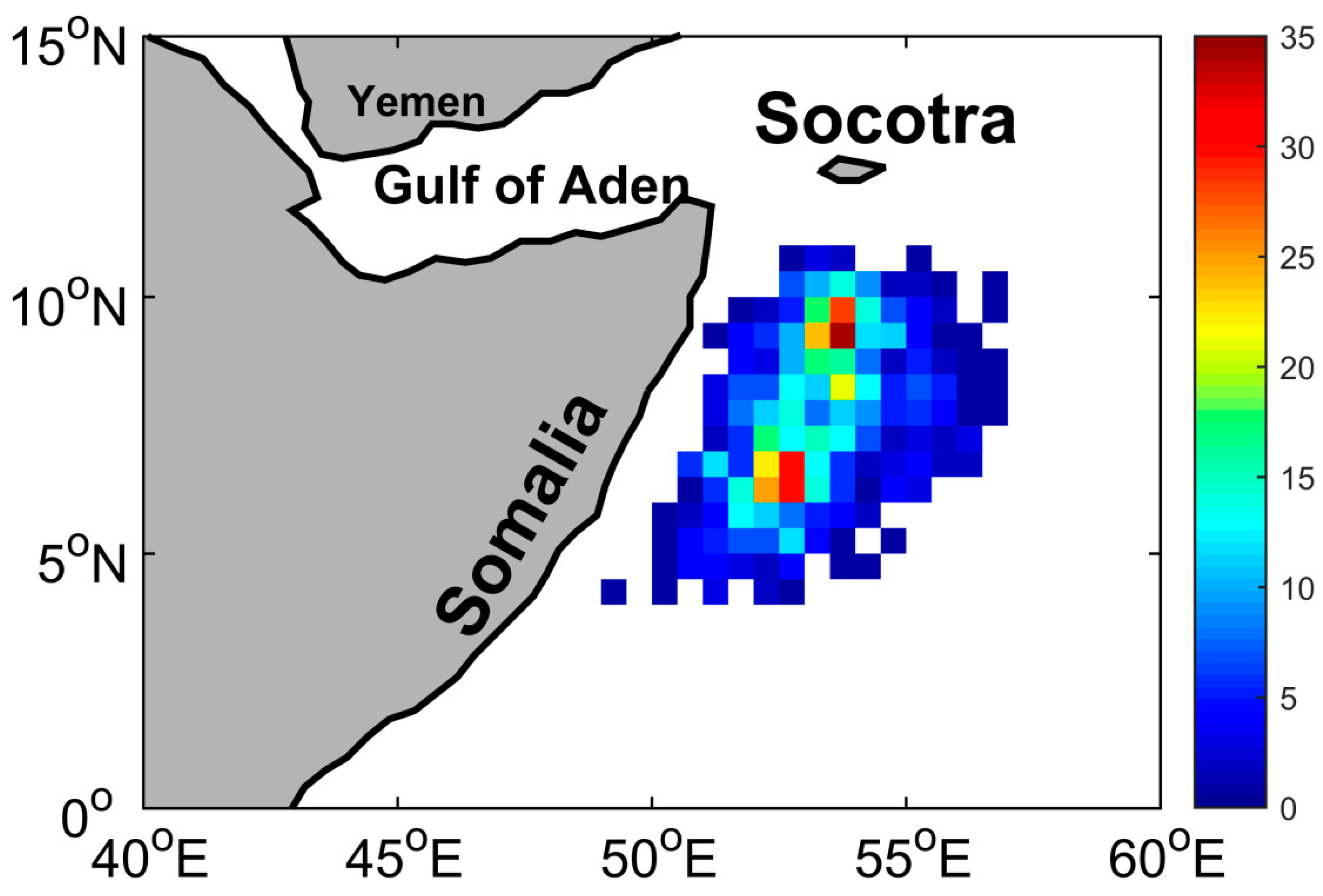
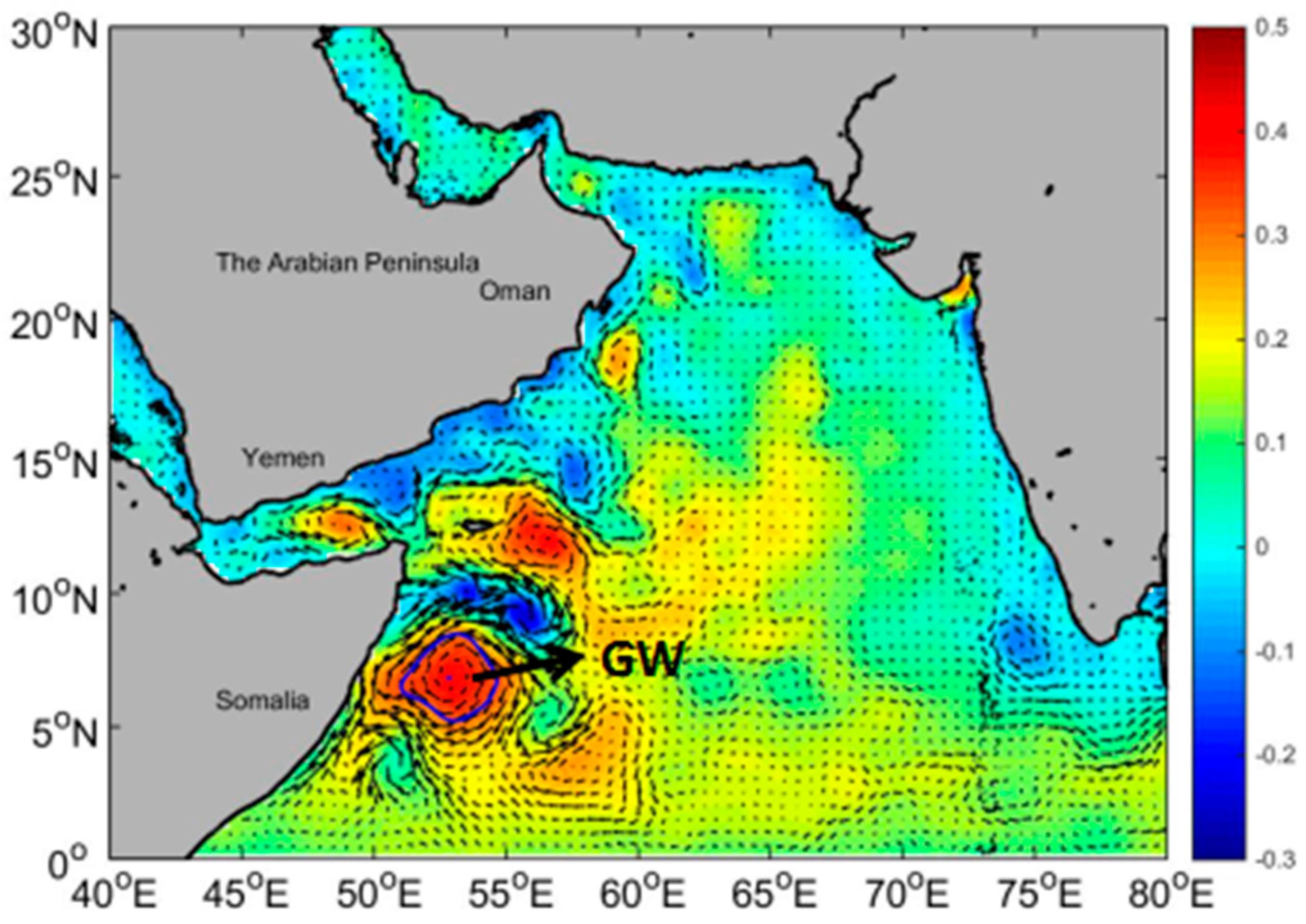
3.1.1. Basic Characteristics

We applied the eddy detection method to the SLA data from 1993 to 2015, and obtained a dataset about the position, radius, lifetime, and intensity of the GW. We used a combination of this dataset, SLA, and SST data to analyze the basic characteristics of the GW in July, when the GW intensity reaches its strongest, shown in Figure 2. Figure 2a shows the SLA distribution within the GW area. In the center of the GW, its maximum value is 0.3 m. The gradient of the SLA is basically the same from west to east, while the gradient is larger in the northern part of the GW than it in the southern part. Figure 2b,c shows the difference of SLA and SST along the latitude from that at the center of the GW, respectively. The farther away from the center, the larger the value of the SLA is. The largest difference appears on the eastern edge, which is about −0.12 m. However, the pattern of SST is different from the SLA. The eddy detection method uses the SLA data to define the GW center, hence, the maximum SLA occurs at the center of the GW, while the maximum SST does not. This phenomenon is attributed to some currents around the GW, which we will discuss in the following section. It can be found that the maximum SST appears on the west side of the GW center. The maximum SST anomaly is −0.7 °C on the eastern edge. The geostrophic velocity calculated based on the SLA profile in Figure 4b is plotted in Figure 4d. At the edge of the GW, the velocity changes slowly, while at the center, the velocity decreases rapidly. The maximum velocity is about 0.45 $\mathrm{m}·{\mathrm{s}}^{-1}$ at the east edge, while the velocity at the west edge is about 0.4 $\mathrm{m}·{\mathrm{s}}^{-1}$.

Monthly mean SLA and associated geostrophic currents from 1993 to 2015 are plotted in Figure 3. It is obvious that there is a positive anomaly center, which is the GW, along the Somali coast from June to October. The intensity of the GW gradually increases in July and August, and weakens in September and October. It can also be seen that there is a westward-propagating Rossby-wave-like signal in the northwest Indian Ocean [31]. A positive SLA begins to form at the southern tip of India in December and arrives on the Somali coast in May, the time matching the formation time of the GW. This is the reason why the Rossby wave propagation is considered to be one mechanism for GW generation. It should be noted that the ‘cyclonic eddy’ signal appearing on the coast of Somalia in January is due to the fact that the AVISO data filters out the multi-year average sea surface height when calculating the SLA, resulting in this false signal in this position in January. This phenomenon is not present in the SST image (not shown).

Figure 4 shows the monthly mean SST (Figure 4a) and SLA (Figure 4c) in the center of the GW from May to October for the period from 1993 to 2015. It can be seen that the SLA increases first and then decreases, while the SST is opposite. This is because the southwest monsoon not only enhances the intensity of the GW, but also enhances upwelling along the coast of Somalia, which upwells the cold seawater. The GW rotates clockwise and rolls up the cold water on the northwest side into the GW, causing the SST inside the GW to decrease. With the weakening of the southwest monsoon, the upwelling on the coast of Somalia gradually weakens, and the SST at the center of the GW begins to increase again.

After the GW enters its maturity, the SLA increases but the SST decreases. It cannot be confirmed whether the overall intensity of the GW increases during this period, so we calculated the mean SST differences (Figure 4b) and SLA differences (Figure 4d) from May to October for the period from 1993 to 2015 (the difference was calculated by using the maximum value minus the minimum value within the GW). The SST anomalies in June, July, August, and September are greater than those during the other two months, which means that the intensity of the GW is relatively stronger during these months, and is the same as the SLA anomalies. The change trend of the SST anomaly is consistent with that of the SLA. Therefore, it can be considered that, under the effect of the southwest monsoon, the GW is strengthened after entering the mature period.

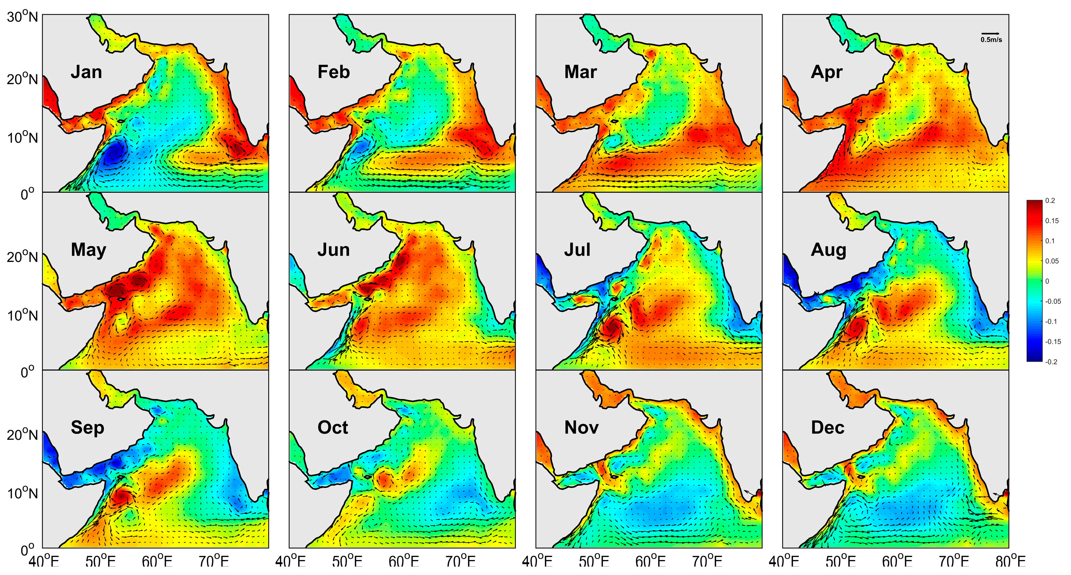
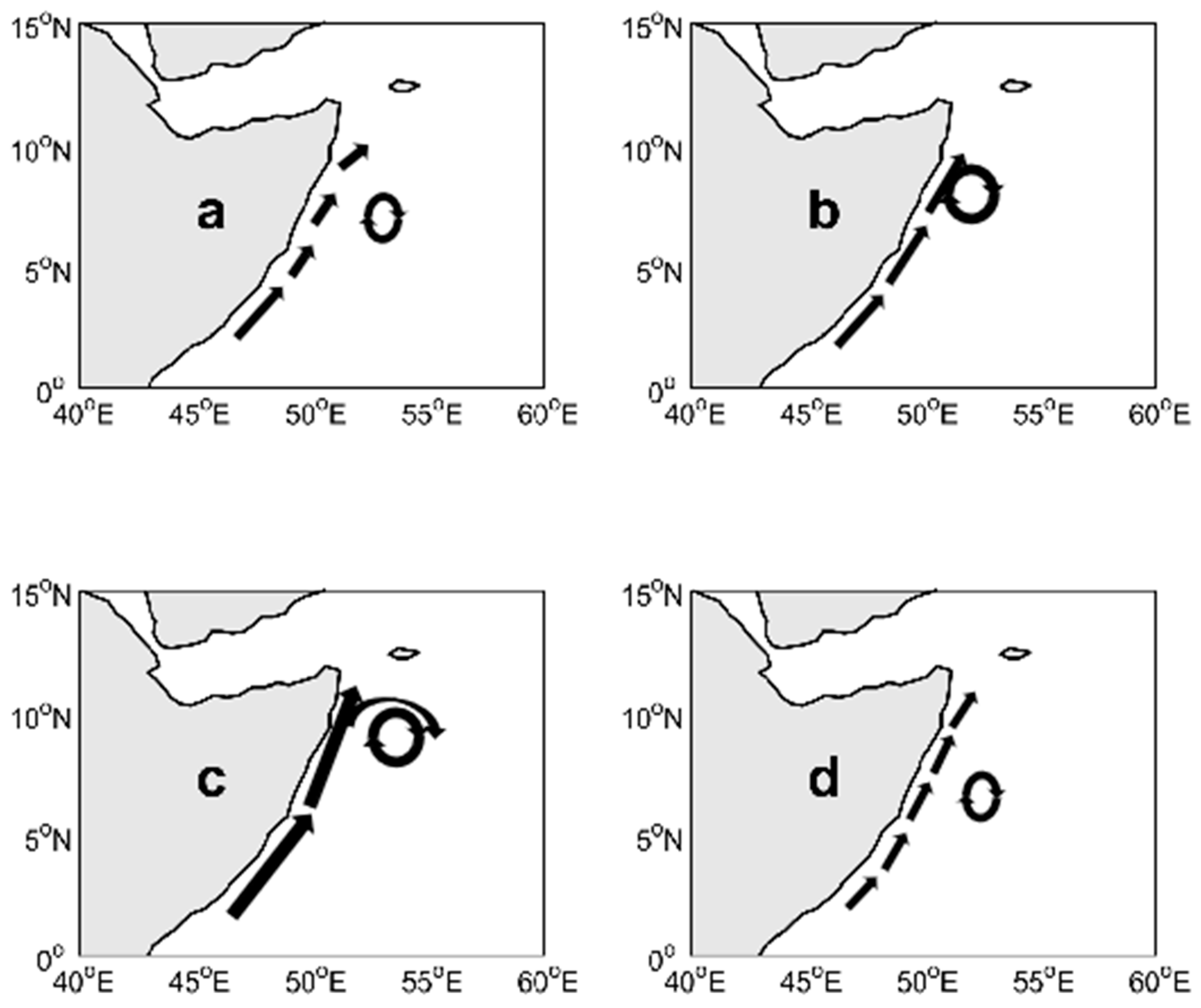
3.1.2. The Movement Pattern

To understand the movement pattern of the GW, we analyzed the trajectories of the GW every year, which is summarized in Figure 5. Before the southwest monsoon onset (May and early June), the velocity of northward flow is small. At this time, the GW is formed, but it is far from the shore (as shown in Figure 5a). After the southwest monsoon onset (June, July, and early August), the velocity of the northward flow begins to increase. At this time, the GW overlaps with the coastal current (as shown in Figure 5b). Under the sustained action of the southwest monsoon (August), the intensity of coastal current reaches its strongest, leading to the bifurcation of the current at its northern end; one branch continues to flow north, and the other branch turns eastward. The GW moves away from the shore and moves southeastward under the action of this eastward flowing branch (as shown in Figure 5c). Finally, when the southwest monsoon disappears (September and October), the northward coastal current also weakens and disappears, and the GW returns to its initial position and eventually disappears (as shown in Figure 5d). It can be found that during this process, the GW presents a clockwise motion.

3.2. Interannual Variations of the GW

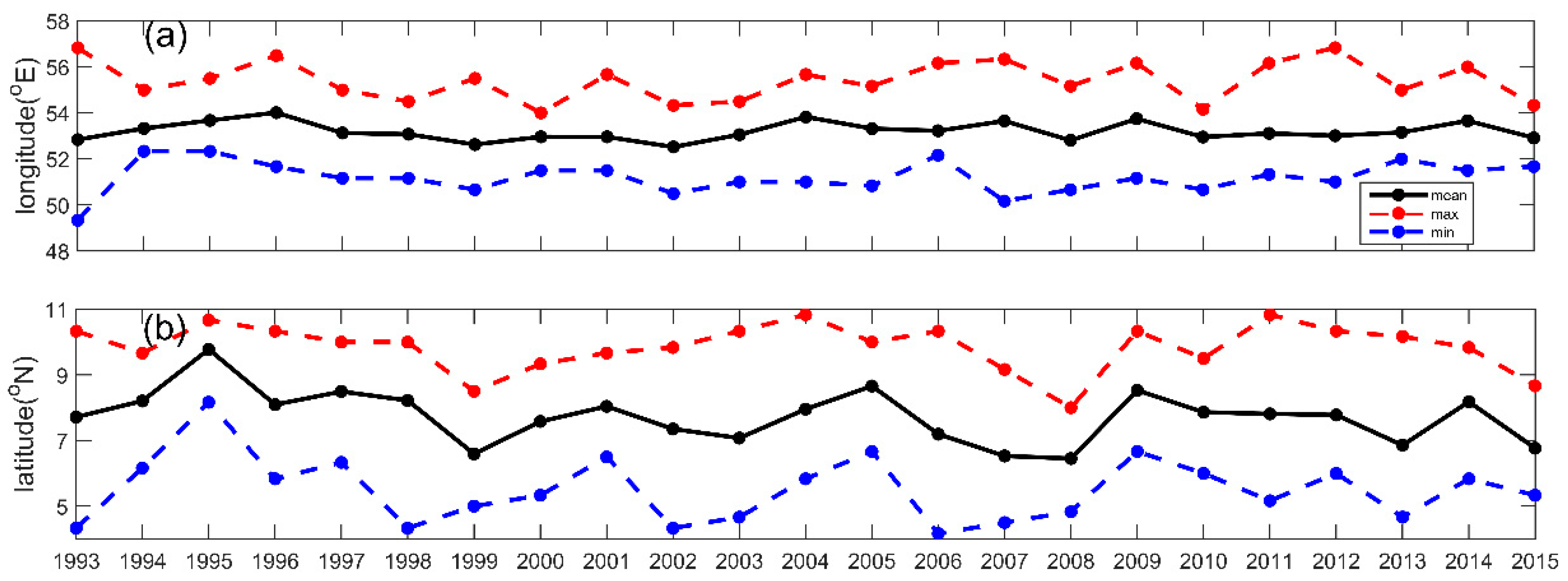
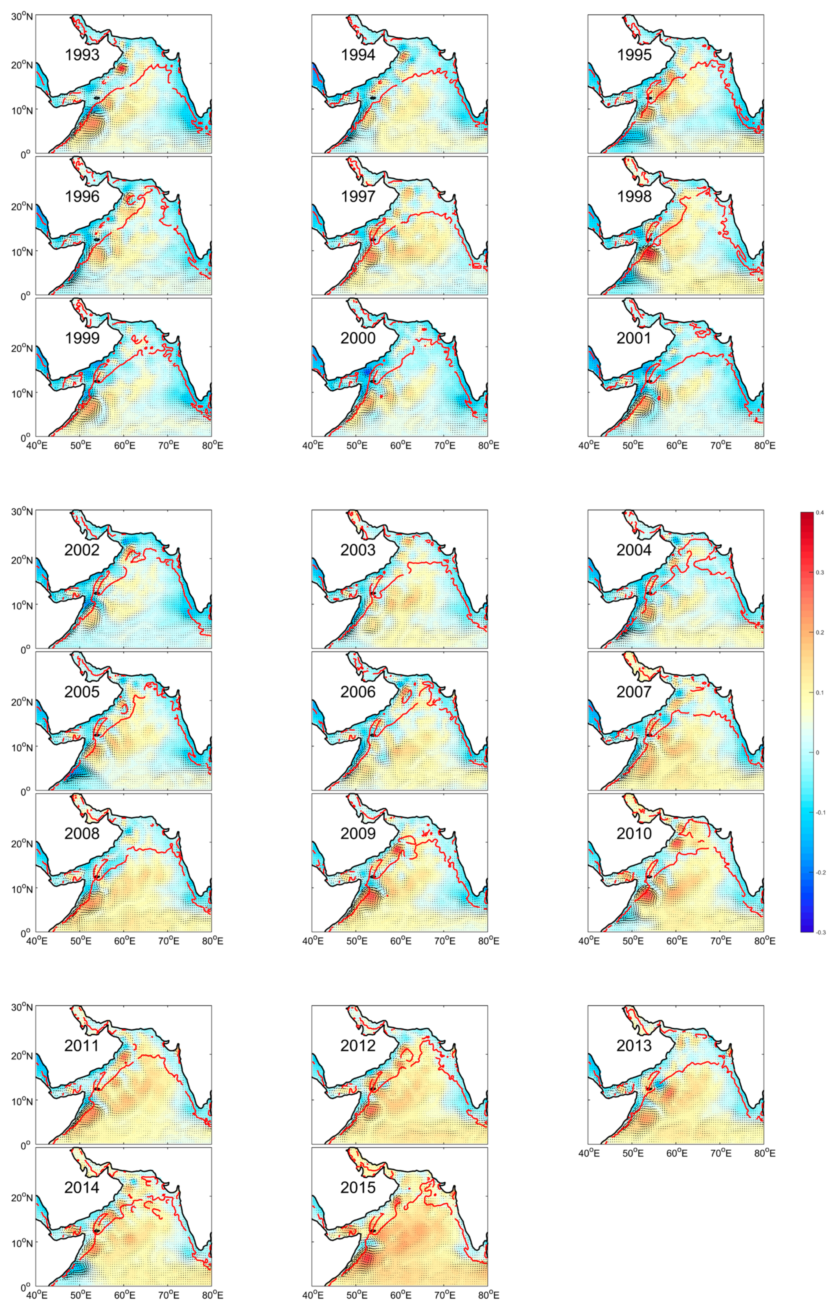
3.2.1. Position

Based on the dataset mentioned above, the locations of the GW centers (latitude and longitude) from 1993 to 2015 and its interannual variation are analyzed in this section. Black lines in Figure 6 are the mean latitudes and longitudes of the GW center every year, and red (blue) lines are the value of the most easterly (westerly) longitudes and the most northerly (southerly) latitudes of the GW center in Figure 6a,b, respectively. The mean position of the GW center is 7.73°N, 53.20°E, the mean value of the most easterly (westerly) longitude is 55.41°E (51.19°E), the mean value of the most northerly (southerly) latitude is 9.86°N (5.51°N), and the moving range of GW center is 4°N–11°N and 49°E–58°E. The mean position of GW reached its most southerly (northerly) point at 6.45°N (9.78°N) in 2008 (1995), and its most easterly (westerly) point at 54.02°E (52.54°E) in 1996 (2002). The maximum and minimum ranges that GW has moved in the longitude direction were 7.5° in 1993 and 2.5° in 2000, respectively, while the maximum and minimum ranges that GW has moved in the latitude direction were 6.17° in 2006 and is 2.5° in 1995, respectively. In addition, it can be observed that the change of the GW position in the east–west direction is smaller than that in the north–south direction. Years when the GW shifted northward were 1993–1998, 2004, 2005, 2009–2012, 2014, and 2015, and years when the GW shifted southward were 1999–2003, 2006–2008, and 2013. In the longitude direction, the GW shifted eastward in 1995, 1996, 2004–2007, 2009, 2014, and 2015, and shifted westward in 1994, 1997–2003, 2008, and 2010–2013. Figure 7 shows the contour of the zero sea surface wind stress curl and the mean state of the GW during the southwest monsoon. The west edge of the GW is tangent to the contour of the zero sea surface wind stress curl in most years, which implies that the interannual variation of the GW position is related to the zero sea surface wind stress curl.

In order to have a more direct view of the GW position variation, the numbers of the GW center presented in bins $0.5°\times 0.5°$ are plotted in Figure 8. It can be seen from Figure 8 that there are two regions where the GW center has occurred the most, one being 53.5°E–54°E, 9°N–10°N, where the GW center occurred 62 times, and the other being 52.5°E–53°E, 6°N–7°N, where the GW center occurred 60 times.

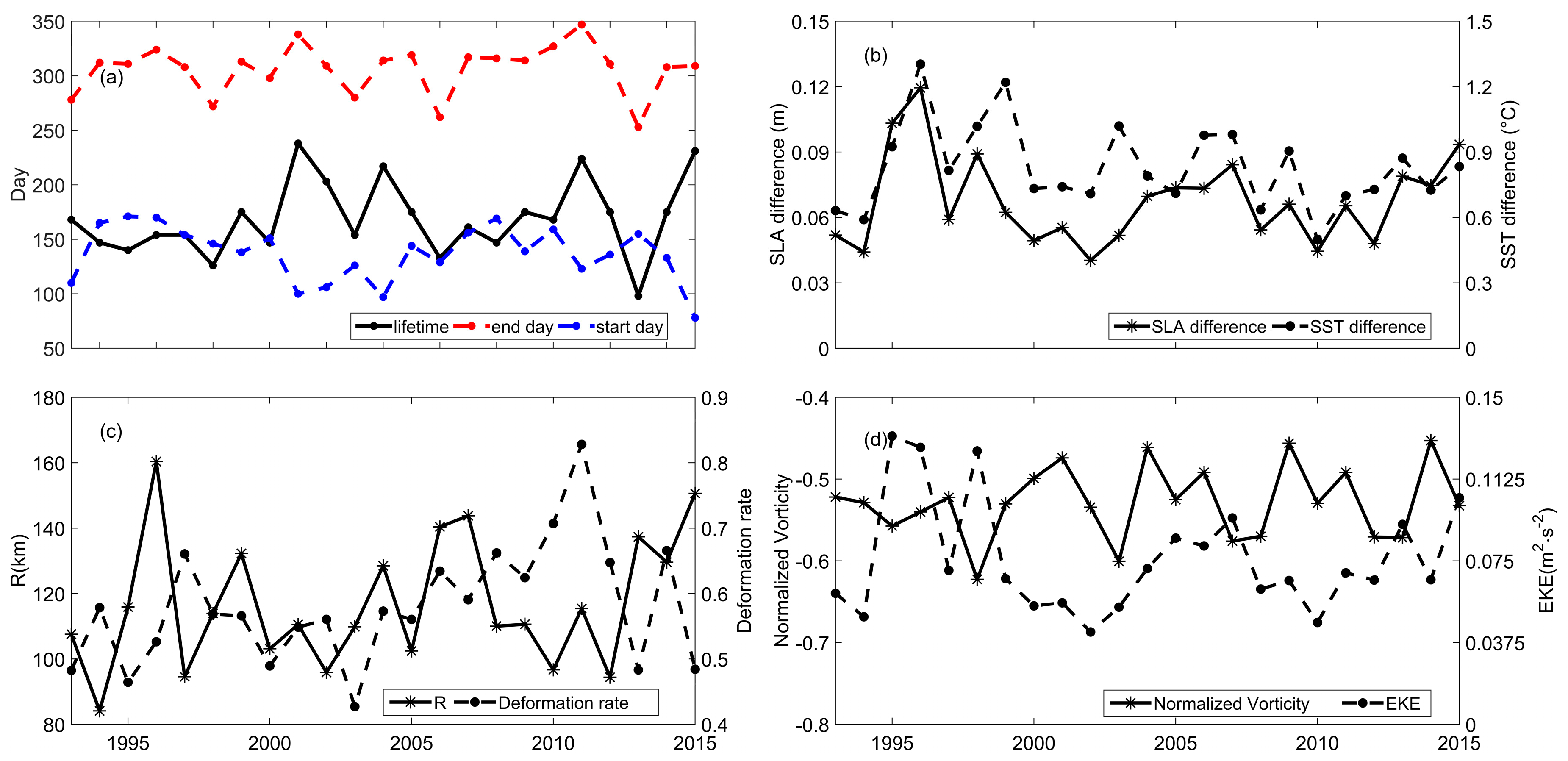
3.2.2. Lifetime

The GW is generated in the early summer, evolves in the following months, and decays in the early winter every year. The start time (blue line), end time (red line), and lifetime (black line) of the GW every year are shown in Figure 9a. The average lifetime of the GW is 169 days. The longest duration occurred in 2001 (238 days), and the shortest duration occurred in 1998 (98 days). The GW has formed at the earliest on 20 March 2015, and the latest on 21 June 1995. It disintegrated the earliest on 20 September 2006, and the latest on 14 December 2011. The lifetime of the GW also exhibits interannual variations; notably, it was relatively shorter with respect to the average from 1993 to 1998 and relatively longer from 1999 to 2005, except for 2003, which displayed a slightly shorter lifetime than the average. Since 2005, the lifetime of the GW has shown shorter and longer alternating transitions every two to three years.

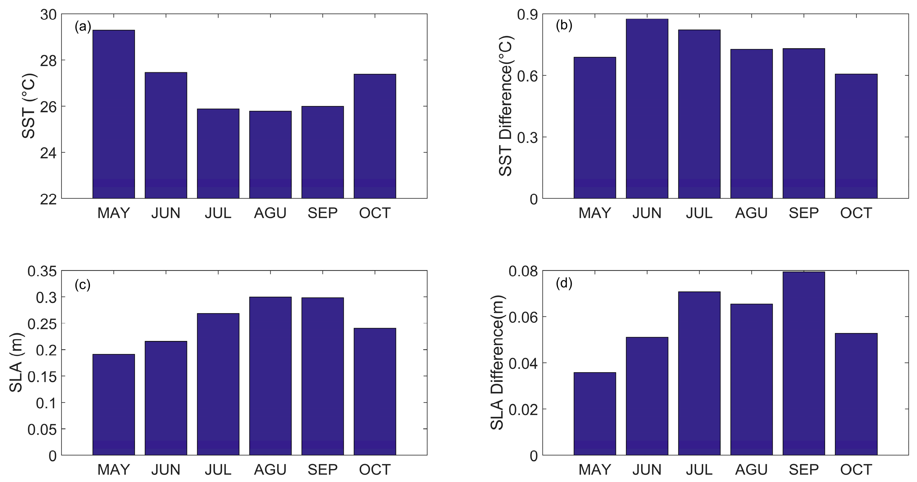
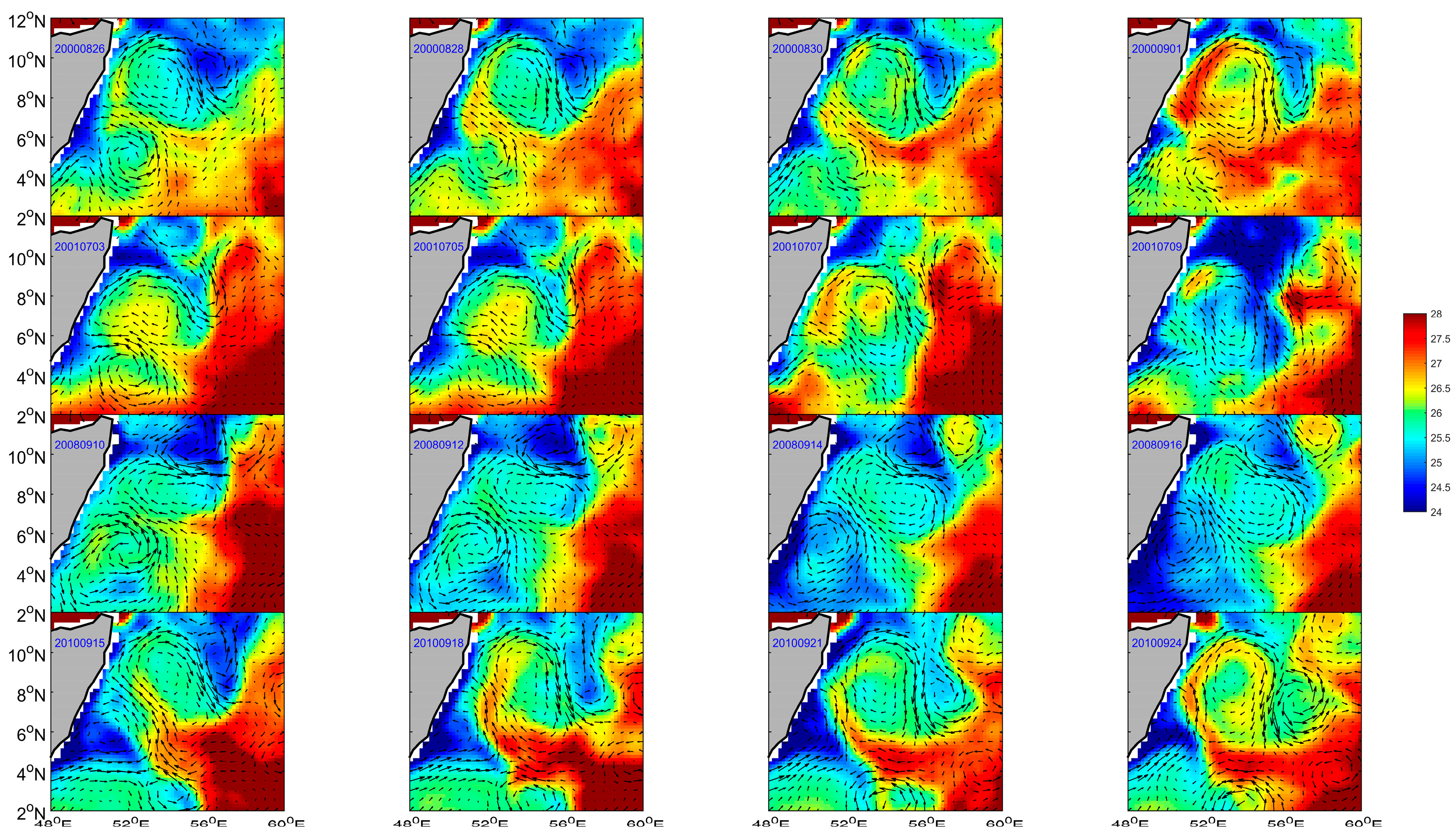
3.2.3. SST and SLA

SST and SLA are two important variables that characterize eddy properties. The SLA difference (solid line) and the SST difference (dotted line) (defined as the maximum minus the minimum within the GW) that represent the intensity of the GW are shown in Figure 9b. It can be found that the mean value of the SLA difference of the GW is 0.07 m. It reaches a maximum value of 0.12 m in 1996 and a minimum value of 0.04 m in 2002. The mean value of the SST difference of the GW is 0.83 °C. The maximum and minimum value are 1.30 °C and 0.50 °C in 1996 and 2010, respectively.

Furthermore, the SLA difference and the SST difference also exhibit obvious interannual variations. Years when the SLA difference is smaller relative to the average are 1993–1994, 1997, 1999–2003 and 2008–2012. Years when the SLA difference is larger relative to the average are 1995–1996, 1998, 2004–2007 and 2013–2015. It can be found that there are more years when the SLA difference is small. Years when the SST difference is smaller relative to the average are 1993–1994, 1997, 2000–2002, 2004–2005, 2008, 2010–2012 and 2014. Years when the SST difference is larger relative to the average are 1995–1996, 1998–1999, 2003, 2006–2007, 2009, 2013 and 2015. It is found that the trends of the SST difference and the SLA difference are basically the same, which indicates that the trends of these two variables can roughly characterize the change of the GW intensity.

3.2.4. Radius, Deformation, Normalized Vorticity, and EKE

In this section, we analyze the radius (Figure 9c), deformation (Figure 9c), the normalized vorticity (Figure 9d), and eddy kinetic energy (EKE) (Figure 9d) of the GW. The radius is defined as the average distance from the GW boundary to the center. The deformation is defined as the ratio of the difference between the long axis and the short axis to the radius. The relative vorticity is the largest in an eddy center and the smallest in the boundary (reaches zero), in theory. The relative vorticity of an eddy is defined as the mean value within the eddy area confined by its boundary [32]. The relative vorticity in Figure 9d is normalized by the planetary rotation. The eddy kinetic energy (EKE) is the mean kinetic energy in the GW coverage area.

In Figure 9c, we can see that the average radius of GW is 116.86 km. The radius in 2015 was the largest, reaching 150.6 km, while it was smallest in 1994, with only 84.1 km. The average deformation rate is 0.58; the largest rate was 0.83 in 2011 and the smallest one was 0.43 in 2003. The radius of GW was smaller in 1993–1995, 1997–1998, 2000–2003, 2005, and 2008–2012, but it was larger in 1996, 1999, 2004, 2006–2007, and 2013–2015. The deformation rate was smaller in 1993–1996, 1998–2005, 2013, and 2015, but it was larger in 1997, 2006–2012, and 2014.

The average normalized vorticity is −0.53; the largest one was −0.62 in 1998 and the smallest one was −0.45 in 2014. The normalized vorticity was smaller in 1994–1996, 1998–1999, 2002–2003, 2007–2008, 2010, 2012–2013, and 2015, but it was larger in 1993, 1997, 2000–2001, 2004–2006, 2009, 2011, and 2014. It can be found that the normalized vorticity changes alternately about every two years.

The average EKE from 1993 to 2015 was 0.08 ${\mathrm{m}}^2·{\mathrm{s}}^{-2}$. In 1996, the EKE of the GW reached a maximum of 0.13 ${\mathrm{m}}^2·{\mathrm{s}}^{-2}$, while it was smallest in 2002 with only $0.04{ \mathrm{m}}^2·{\mathrm{s}}^{-2}$. The EKE was smaller in 1993–1994, 1997, 1999–2004, 2008–2012, and 2014, but it is larger in 1995–1996, 1998, 2005–2007, 2013, and 2015. By comparing the radius and the EKE of the GW, we can find that their variations are similar, and the correlation coefficient between these two quantities is 0.60.

3.3. Atmospheric Responses to the GW

The GW is a seasonal mesoscale eddy occurring in the western Indian Ocean, close to the east coast of Africa. It is bound to have a certain impact on the countries bordering this area. Seo et al. [23] and Seo [24] used an air–sea coupled model to examine the GW’s effect on the atmosphere. Here, we have applied the observation product and reanalyzed data to further explore the issue. For the composite analysis done in this section, a 4° × 4° square was selected by taking 2° in each of the four directions, moving from the center of the GW. The small-scale characteristics of the variables were then obtained by removing an 8° zonal moving average from them.

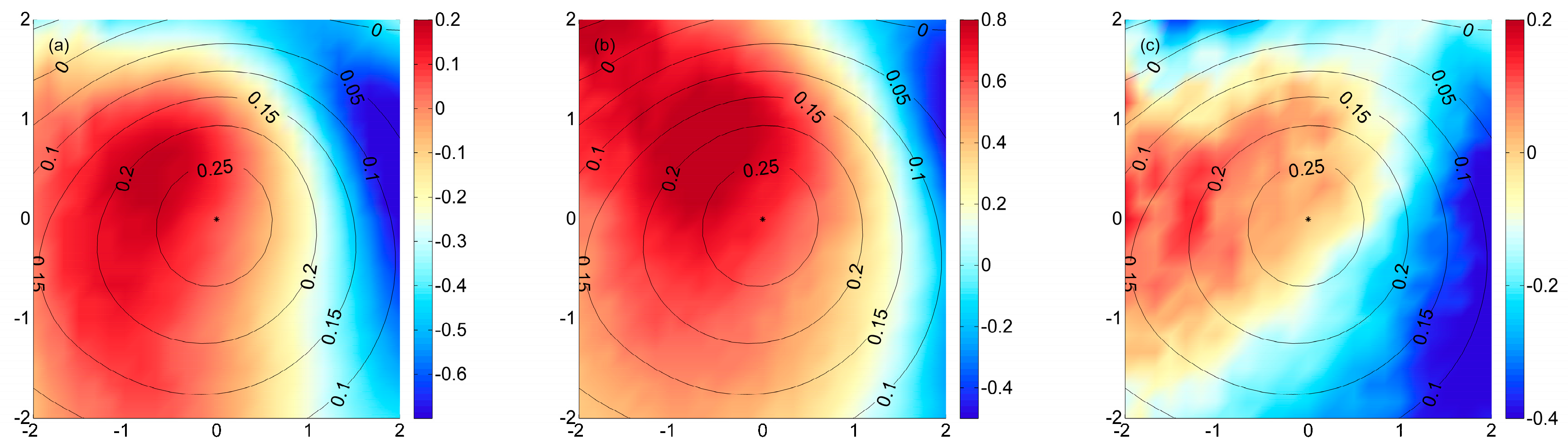
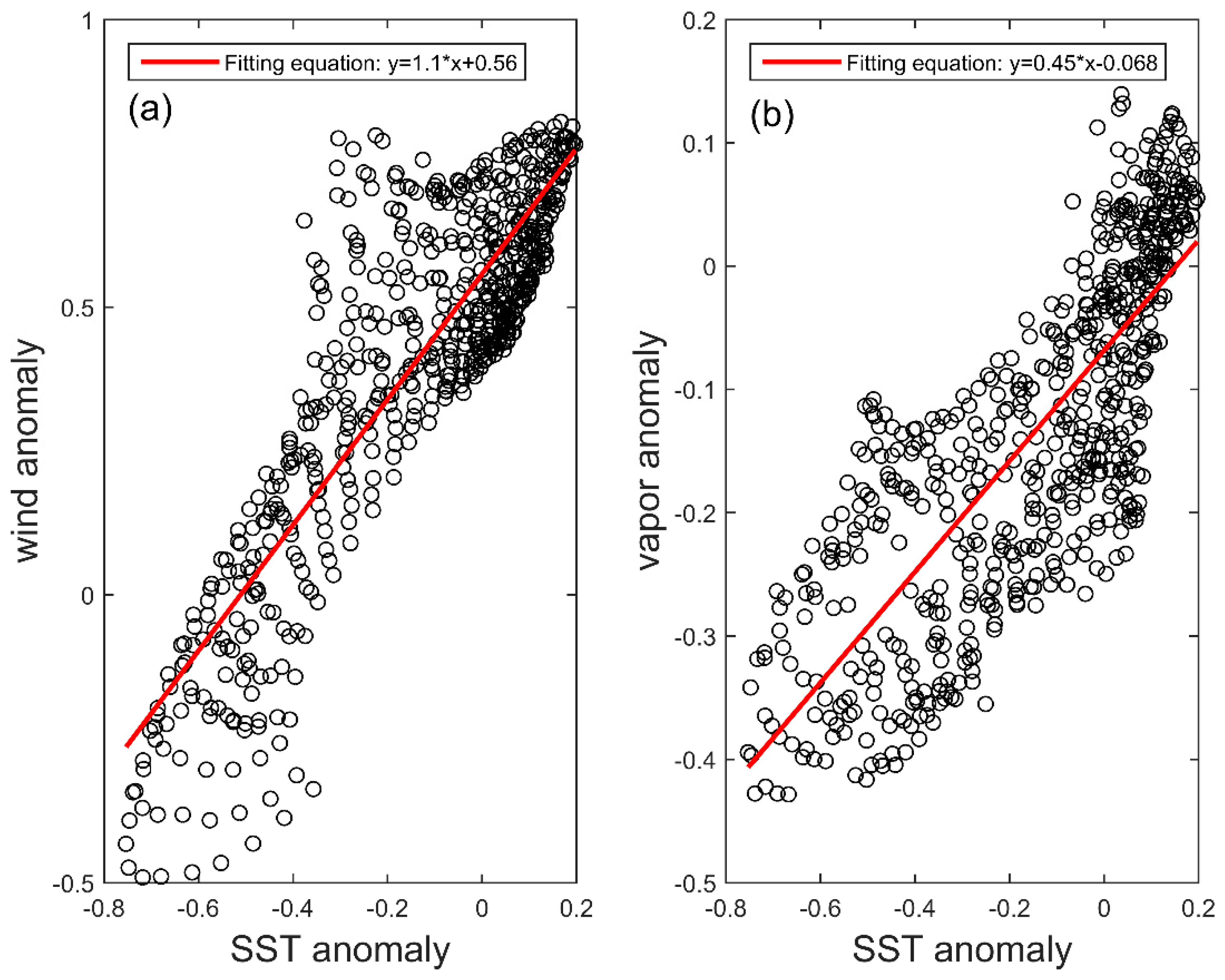
3.3.1. Composite Results near the Sea Surface

Composites of the SST, wind, and water vapor anomalies are shown in Figure 10. The position of the maximum SST anomaly (0.2 °C) does not coincide with the center of the GW, but shifts toward the northwest (Figure 10a). Figure 11 shows four evolution processes of the SST and flow fields near the GW as examples to explain this phenomenon. Climatologically, the SST is relatively higher on the southeast of the GW. Under the influence of the GW, the warmer seawater moves toward the south of the GW, and gradually moves to the west and northwest of the GW. The example of August 2000 (Figure 11, the first row) is analyzed in detail. On August 26, warm water near 56$°\mathrm{E}$, 6$°\mathrm{N}$ gradually moved toward the northwest; on August 28, the SST on the southwest side of the GW was about 0.5 °C higher than that of two prior, and warm water still moved along the GW; on August 30, the SST on the southwest side of the GW further increased; on 1 September, the SST on the west side and the northwest side of the GW was about 1 °C higher than the previous days, and the earliest batch of warm water had reached the east side of the GW. Throughout the process, the cold Somali coastal current, which locates on the west side of the GW, flowed to the east side of the GW. Therefore, the SST on the northwest and south side of the GW was always higher than that on the east side, which explains why the largest positive SST anomaly center in Figure 10a appeared on the northwest side of the GW. The evolution processes of the other three examples (Figure 11, the second to the fourth row) are basically consistent with the example of August 2000. Although the temperature of the warm water reaching the west side of the GW in these three examples is not as high as that in 2000, they also show a similar pattern: that the SST on the west side of the GW is higher than that on the east side.

The maxima of the wind speed anomalies (Figure 10b) and the water vapor anomalies (Figure 10c) are also located on the northwest side of the GW center. The pattern of the wind speed anomaly is similar to that of the SST anomaly, and the water vapor shows a positive anomaly on the northwest side of the GW and a negative anomaly on the southeast side of the GW. The offset of these two anomaly centers with the GW center is affected by the SST. Previous studies have shown that wind accelerates over warm water at frontal or eddy scale [15,20]. The center of the wind anomaly well matches the center of SST anomaly. The water vapor is mainly affected by wind and temperature. High wind speed and temperature accelerate the evaporation of seawater. Therefore, positive water vapor anomalies also occur over warm SST at small scales.

In order to understand exactly how large the influence of the SST anomaly on the wind speed and the water vapor anomalies is, scatter plots of the SST, wind, and water vapor anomaly are plotted and linear fit was performed (Figure 12a,b). The fitting coefficient between the SST and wind speed anomalies is 1.1, indicating that, corresponding to 1 °C increases of the SST, the wind speed increases by about 1.1 $\mathrm{m}·{\mathrm{s}}^{-1}$. Similarly, the fitting coefficient between the SST and water vapor anomalies is 0.45, indicating that water vapor increases by about 0.45 mm in response to 1 °C increases in the SST.

3.3.2. Composite Results in the Vertical Direction

In addition to analyzing variables in the horizontal direction, composites of the vertical velocity ($\mathsf{\omega }$) anomalies (Figure 13a,b), vertical transport anomalies of transient zonal momentum (Figure 13c,d), and wind speed anomalies (Figure 13e,f) were also analyzed using the ERA reanalysis data.

In Figure 13b, a positive anomaly center of the vertical velocity can be seen over the west side of the GW center, which means that there is anomalous subsidence extending up as high as 800 hPa. The maximum vertical velocity anomaly is at 900 hPa. The negative vertical velocity anomalies occur over the east side of GW center, which means that there is anomalous ascending, and extend up to the same level as the positive anomalies. In Figure 13a, the positive anomaly area gradually increases as the latitude increases, and the farther away from the center of the GW, the smaller the value of the positive anomaly is.

The vertical transport anomalies of transient zonal momentum are represented by $\overline{u^{\prime }{\omega }^{\prime }}$. The 31 point bandpass filter was used to estimate $u^{\prime }$ and ${\omega }^{\prime }$. In Figure 13d, the positive anomalies occurred over the west of the GW center from the sea surface to 800 hPa, and negative anomalies occurred in the east side, the same as the positive anomalies. Like the vertical velocity anomalies, the maximum anomalies and minimum anomalies also appeared at 900 hPa. The positive value represents downward transport of transient zonal momentum, which can accelerate the wind speed in lower levels, and the negative value is opposite. This result of the vertical transport anomalies of transient zonal momentum is different from that of Ma et al. [21]. Compared with their study, the positive anomalies shifted to the west side of the eddy center, with negative anomalies in the lower atmosphere. This may arise from regional differences.

Figure 13e and f shows the wind speed anomaly in the vertical direction. It is different from the vertical velocity and $\overline{u^{\prime }{\omega }^{\prime }}$, with the maximum positive and the minimum negative wind speed anomaly appearing at 950 hPa. In Figure 13e, the positive wind speed anomaly appears northwest of the GW center, consistent with previous horizontal composite results. The downward transport of transient zonal momentum exited on the west side of the GW center, which resulted in the wind speed acceleration on the west side of the GW. The maximum vertical transport anomalies of transient zonal momentum was 900 hPa. Therefore, the maximum wind speed anomaly appeared at a lower height, which explains why the largest positive anomaly occurred at 950 hPa.

Through the composite analysis of the horizontal and the vertical directions, we can summarize the effects of the GW on the atmosphere. The SST is higher on the west side of the GW than on the east side, so the wind speed near the sea surface on the west side of the GW is faster. Under the joint action of the SST and wind, positive water vapor anomalies also occur on the west side of the GW. In the vertical direction, both the downward movement and downward transport of transient zonal momentum on the west side of the GW can accelerate the wind speed in lower levels. It can be seen that both the SST and upper atmosphere can accelerate the wind speed on the west side of the GW.

4. Summary and Discussion

This study mainly focuses on the mean state and the interannual variations of the GW, and discusses the corresponding atmospheric responses.

Based on the eddy dataset, SLA, and SST data, we analyzed the basic characteristics of the GW in July. We found that the maximum SLA was 0.3 m in the center of the GW, the largest SLA (SST) difference was −0.12 m (−0.7 °C), and the maximum velocity was about 0.45 $\mathrm{m}·{\mathrm{s}}^{-1}$ at the edge of the GW. By analyzing the monthly mean SLA and geostrophic currents, we found that the GW is presented from June to October, and the time when the Rossby wave arrives on the coast of Somalia basically coincides with the formation time of the GW. It can be suggested that the Rossby wave plays an important role in the GW generation. By analyzing the SST difference and SLA difference from May to October, we can conclude that the intensity of the GW is enhanced during the southwest monsoon. From Argo and WOA data, we consider that the effect of the GW can reach 300 m below the sea surface.

The average position of the GW center was 7.73°N, 53.20°E, and the mean lifetime, radius, normalized vorticity, EKE, and deformation rate were 169 days, 116.86 km, −0.53, 0.08 ${\mathrm{m}}^2·{\mathrm{s}}^{-2}$, and 0.58, respectively, during the period of 1993–2015. In addition, we carried out a detailed analysis of the interannual variation characteristics of variables related to the GW, namely, center position, the SST difference, the SLA difference, radius, deformation, normalized vorticity, and EKE: they all exhibit clear interannual variations.

We used composite analysis to study the response of the atmosphere to the GW, and found that the centers of the maximum anomaly of the SST, wind speed, and water vapor were all on the northwest side of the GW. Factors contributing to such a result include that the SST on the west side of the GW is higher than that on the east side, under the influence of the GW. In the vertical direction, we found that three variables have the same mode. The positive and negative anomaly centers of vertical velocity and vertical transport anomalies of transient zonal momentum were observed at 900 hPa, while the positive and negative wind speed anomaly center appeared at 950 hPa.

The basic characteristics of the GW obtained by the present study agree with previous investigations of the topic. Compared with previous studies on the GW, we have conducted an extensive investigation of the interannual variation and the impacts of the GW on the atmospheric boundary layer. The GW variation was not found to be well related to basin-scale variations such as the IOD index or ENSO events, but the western edge of the GW does move along the contour of the zero sea surface wind stress curl. The relationship between local variation of the GW and basin-scale variation needs to be further investigated. Due to the availability of the observational data, the detailed physical processes on how the GW impacts on the atmosphere are not clear. We will apply air–sea coupling models to explore the issue in the near future.

References

- Schott, F.; Mccreary, J.P. The monsoon circulation of the Indian Ocean. Prog. Oceanogr. 2001, 51, 1–123. [Google Scholar] [CrossRef]
- Schott, F. Monsoon response of the Somali Current and associated upwelling. Prog. Oceanogr. 1983, 12, 357–381. [Google Scholar] [CrossRef]
- Swallow, J.C.; Fieux, M. Historical evidence for two gyres in the Somali Current. J. Mar. Res. 1982, 40, 747–755. [Google Scholar]
- Bruce, J.G. Eddies off the Somali Coast during the Southwest Monsoon. J. Geophys. Res.-Oceans 1979, 84, 7742–7748. [Google Scholar] [CrossRef]
- Bruce, J.; Fieux, M.; Gonella, J. A note on the continuance of the Somali eddy after the cessation of the Southwest monsoon. Oceanol. Acta 1981, 4, 7–9. [Google Scholar]
- Beal, L.M.; Donohue, K.A. The Great Whirl: Observations of its seasonal development and interannual variability. J. Geophys. Res.-Oceans 2013, 118, 1–13. [Google Scholar] [CrossRef]
- Beal, L.M.; Hormann, V.; Lumpkin, R.; Foltz, G.R. The Response of the Surface Circulation of the Arabian Sea to Monsoonal Forcing. J. Phys. Oceanogr. 2014, 43, 2008–2022. [Google Scholar] [CrossRef]
- McCreary, J.; Kundu, P. A numerical investigation of the Somali Current during the Southwest Monsoon. J. Mar. Res. 1988, 46, 25–58. [Google Scholar] [CrossRef]
- Jensen, T.G. Modeling the seasonal undercurrents in the Somali Current system. J. Geophys. Res.-Oceans 1991, 96, 22151–22167. [Google Scholar] [CrossRef]
- Vic, C.; Roullet, G.; Carton, X.; Capet, X. Mesoscale dynamics in the Arabian Sea and a focus on the Great Whirl life cycle: A numerical investigation using ROMS. J. Geophys. Res.-Oceans 2015, 119, 6422–6443. [Google Scholar] [CrossRef]
- Cao, Z.; Hu, R. Research on the interannual variability of the Great Whirl and the related mechanisms. J. Ocean Univ. China 2015, 14, 17–26. [Google Scholar] [CrossRef]
- Luther, M.E.; O’Brien, J.J. Modelling the Variability in the Somali Current. Elsevier Oceanogr. Ser. 1989, 50, 373–386. [Google Scholar] [CrossRef]
- Luther, M.E. Interannual variability in the Somali Current 1954–1976. Nonlinear Anal. 1999, 35, 59–83. [Google Scholar] [CrossRef]
- Wirth, A.; Willebrand, J.; Schott, F. Variability of the Great Whirl from Observations and Models; Deep-Sea Research Part II; Elsevier: Amsterdam, The Netherlands, 2002; Volume 49, pp. 1279–1295. [Google Scholar] [CrossRef]
- Vecchi, G.A.; Xie, S.P.; Fischer, A.S. Ocean–Atmosphere Covariability in the Western Arabian Sea. J. Clim. 2004, 17, 1213–1224. [Google Scholar] [CrossRef]
- Nonaka, M.; Xie, S.P. Covariations of Sea Surface Temperature and Wind over the Kuroshio and Its Extension: Evidence for Ocean-to-Atmosphere Feedback. J. Clim. 2003, 16, 1404–1413. [Google Scholar] [CrossRef]
- Mafimbo, A.J.; Reason, C.J.C. Air-sea interaction over the upwelling region of the Somali coast. J. Geophys. Res.-Oceans 2010, 115, 152–162. [Google Scholar] [CrossRef]
- Chelton, D.B.; Schlax, M.; Freilich, H.H.; Milliff, R.F. Satellite measurements reveal persistent small-scale features in ocean winds. Science 2004, 303, 978–983. [Google Scholar] [CrossRef]
- Koseki, S.; Watanabe, M. Atmospheric boundary layer response to mesoscale SST anomalies in the Kuroshio Extension. J. Clim. 2010, 23, 2492–2507. [Google Scholar] [CrossRef]
- Frenger, I.; Gruber, N.; Knutti, R.; Münnich, M. Imprint of Southern Ocean eddies on winds, clouds and rainfall. Nat. Geosci. 2013, 6, 608–612. [Google Scholar] [CrossRef]
- Ma, J.; Xu, H.; Dong, C.; Lin, P.; Liu, Y. Atmospheric responses to oceanic eddies in the Kuroshio Extension region. J. Geophys. Res.-Atmos. 2015, 120, 6313–6330. [Google Scholar] [CrossRef]
- Ma, J.; Xu, H.; Dong, C. Seasonal variations in atmospheric responses to oceanic eddies in the Kuroshio Extension. Tellus A 2016, 68, 31563. [Google Scholar] [CrossRef]
- Seo, H.; Murtugudde, R.; Jochum, M.; Miller, A.J. Modeling of mesoscale coupled ocean-atmosphere interaction and its feedback to ocean in the western Arabian Sea. Ocean Model. 2008, 25, 120–131. [Google Scholar] [CrossRef]
- Seo, H. Distinct influence of air-sea interactions mediated by mesoscale sea surface temperature and surface current in the Arabian Sea. J. Clim. 2017, 30, 8061–8080. [Google Scholar] [CrossRef]
- Ducet, N.; Traon, P.Y.; Reverdin, G. Global high-resolution mapping of ocean circulation from TOPEX/Poseidon and ERS-1 and-2. J. Geophys. Res. 2000, 105, 19477–19498. [Google Scholar] [CrossRef]
- Reynolds, R.W.; Smith, T.M.; Liu, C.; Chelton, D.B.; Casey, K.S.; Michael, G. Daily high-resolution-blended analyses for sea surface temperature. J. Clim. 2007, 20, 5473–5496. [Google Scholar] [CrossRef]
- Sun, W.; Dong, C.; Tan, W.; He, Y. Statistical Characteristics of Cyclonic Warm-Core Eddies and Anticyclonic Cold-Core Eddies in the North Pacific Based on Remote Sensing Data. Remote Sens. 2019, 11, 208. [Google Scholar] [CrossRef]
- Wentz, F.J.; Gentemann, C.; Smith, D.; Chelton, D. Satellite measurements of sea surface temperature through clouds. Science 2000, 288, 847–850. [Google Scholar] [CrossRef]
- The ERA-Interim reanalysis: Configuration and performance of the data assimilation system. Q. J. R. Meteorol. Soc. 2011, 137. [CrossRef]
- Nencioli, F.; Changming, D.; Dickey, T.; Washburn, L.; McWilliams, J.C. A Vector Geometry–Based Eddy Detection Algorithm and Its Application to a High-Resolution Numerical Model Product and High-Frequency Radar Surface Velocities in the Southern California Bight. J. Atmos. Ocean. Technol. 2010, 27, 564. [Google Scholar] [CrossRef]
- Subrahmanyam, B.; Robinson, I.S.; Rblundell, J.; Challenor, P. Indian Ocean Rossby waves observed in TOPEX/POSEIDON altimeter data and in model simulations. Int. J. Remote Sens. 2001, 22, 141–167. [Google Scholar] [CrossRef]
- Dong, C.; Lin, X.; Liu, Y.; Nencioli, F.; Chao, Y.; Guan, Y.; McWilliams, J.C. Three-dimensional oceanic eddy analysis in the Southern California Bight from a numerical product. J. Geophys. Res.-Oceans 2012, 117, 92–99. [Google Scholar] [CrossRef]
© 2019 by the authors. Licensee MDPI, Basel, Switzerland. This article is an open access article distributed under the terms and conditions of the Creative Commons Attribution (CC BY) license (http://creativecommons.org/licenses/by/4.0/).
Share and Cite
Wang, S.; Zhu, W.; Ma, J.; Ji, J.; Yang, J.; Dong, C. Variability of the Great Whirl and Its Impacts on Atmospheric Processes. Remote Sens. 2019, 11, 322. https://doi.org/10.3390/rs11030322
Wang S, Zhu W, Ma J, Ji J, Yang J, Dong C. Variability of the Great Whirl and Its Impacts on Atmospheric Processes. Remote Sensing. 2019; 11(3):322. https://doi.org/10.3390/rs11030322
Chicago/Turabian StyleWang, Sen, Weijun Zhu, Jing Ma, Jinlin Ji, Jingsong Yang, and Changming Dong. 2019. "Variability of the Great Whirl and Its Impacts on Atmospheric Processes" Remote Sensing 11, no. 3: 322. https://doi.org/10.3390/rs11030322
APA StyleWang, S., Zhu, W., Ma, J., Ji, J., Yang, J., & Dong, C. (2019). Variability of the Great Whirl and Its Impacts on Atmospheric Processes. Remote Sensing, 11(3), 322. https://doi.org/10.3390/rs11030322