Daily River Discharge Estimation Using Multi-Mission Radar Altimetry Data and Ensemble Learning Regression in the Lower Mekong River Basin

Abstract

Estimating river discharge (Q) is critical for ecosystems and water resource management. Traditionally, estimating Q has depended on a single rating curve or the Manning equation. In contrast to the single rating curve, several rating curves at different locations have been linearly combined in an ensemble learning regression method to estimate Q (ELQ) at the Brazzaville gauge station in the central Congo River in a previous study. In this study, we further tested the proposed ELQ and apply it to the Lower Mekong River Basin (LMRB) with three locations: Stung Treng, Kratie, and Tan Chau. Two major advancements for estimating Q with ELQ are presented. First, ELQ successfully estimated Q at Tan Chau, downstream of Kratie, where hydrodynamic complexities exist. Since the hydrologic characteristics downstream of Kratie are extremely diverse and complex in time and space, most previous studies have estimated Q only upstream from Kratie with hydrologic models and statistical methods. Second, we estimated Q over the LMRB using ELQ with water levels (H) obtained from two radar altimetry missions, Envisat and Jason-2, which made it possible to estimate Q seamlessly from 2003 to 2016. Owing to ELQ with multi-mission radar altimetry data, we have overcome the problems of a single rating curve: Locations for estimating Q have to be close to virtual stations, e.g., a few tens of kilometers, because the performance of the single rating curve degrades as the distance between the location of Q estimation and a virtual station increases. Therefore, most previous studies had not used Jason-2 data whose cross-track interval is about 315 km at the equator. On the contrary, several H obtained from Jason-2 altimetry were used in this study regardless of distances from in-situ Q stations since the ELQ method compensates for degradation in the performance for Q estimation due to the poor rating curve with virtual stations away from in-situ Q stations. In general, the ELQ-estimated Q (${\widehat{Q}}_{ELQ}$) showed more accurate results compared to those obtained from a single rating curve. In the case of Tan Chau, the root mean square error (RMSE) of ${\widehat{Q}}_{ELQ}$ decreased by 1504/1338 m³/s using Envisat-derived H for the training/validation datasets. We successfully applied ELQ to the LMRB, which is one of the most complex basins to estimate Q with multi-mission radar altimetry data. Furthermore, our method can be used to obtain finer temporal resolution and enhance the performance of Q estimation with the current altimetry missions, such as Sentinel-3A/B and Jason-3.

1. Introduction

Inland freshwater is regarded as an essential resource for ecosystems, yet we still have limited knowledge of river discharge (Q) variation due to its heterogeneities in time and space [1,2]. The number of gauging stations has declined primarily due to reductions in government funding for the maintenance of stream gauges [3]. Instead, studies on the estimation of Q have emerged using hydraulic variables (water levels, inundation areas, river widths, and surface water slopes) obtained from remote sensing with a multiplicative method [4,5], such as the Manning equation [6] or a rating curve generated by comparing those hydraulic variables from remote sensing with in-situ Q measurements [7,8]. However, those methods require multiple hydraulic variables that may not be available everywhere or depend on rating curves (at-a-station hydraulic geometry, AHG) [9] that vary with high and low water seasons [10,11,12,13].

Recently, Kim et al. [14] introduced the ensemble learning regression for estimating Q (termed ELQ), which has been proven to be an effective method compared to previous methods based on a single rating curve. Details about ELQ can be found in [14]. Its essence is that ELQ, a machine learning method, trains each base learner individually and then combines them linearly. In other words, ELQ generates several base learners, e.g., rating curves, at different locations and combines and harmonizes them using a data-driven approach. As such, ELQ has the potential to create a more accurate function to estimate Q. A brief review of ensemble learning regression and ELQ will be presented in Section 3.

Kim et al. [14] showed that ELQ could generate a strong Q estimation model using altimetry-derived water levels (hereafter “altimetry-derived water levels” are referred to as “H”) obtained at two or three different virtual stations. A virtual station (VS) is defined as a location where a ground track of satellite altimetry overpasses a waterbody [15,16]. Traditionally, AHG is used at a specific location and is not transferable to other sites, whereas ELQ can integrate observations at different locations.

Although ELQ is a novel method to estimate Q, it still requires in-situ Q data in order to train the base learners and obtain their weights [14]. Note that Kim et al. [17] applied ELQ to estimate Q from 2003 to 2010 using H and the hydrologic-hydraulic hillslope river routing (HRR) model without the aid of in-situ Q over the central Congo River. However, the HRR model used in [17] was parameterized and compared to mean monthly streamflow determined from the historical Q data from 1903 to 1990. Moreover, ELQ has been applied only to the central Congo River basin in [14,17], and their studies only estimated Q at a single location, the Kinshasa-Brazzaville station (Lat/Lon: 4.2822°S/15.3008°E).

On the other hand, the hydraulic complexities in the Lower Mekong River Basin (LMRB) hinder accurate estimation of Q. One of these complexities is due to the existence of Tonle Sap Lake (TSL, see Figure 1 for its location). The TSL is the largest body of freshwater in Southeast Asia, and it has a crucial role for Cambodia’s food supply and flood control as a natural reservoir [18]. The TSL has a flow reversal between the wet and dry seasons. The Mekong River flows from the mainstem into the TSL during the wet season (May/June to October/November) while the river flows from the TSL into the mainstem during the dry season (October/November to May/June) [18,19]. The Mekong River Commission (MRC) [18] in 2005 (p.49) describes the difficulty in estimating Q in the LMRB as:

“Downstream from Kratie, seasonal floodplain storage dominates the annual regime and there is significant movement of water between channels over flooded areas, the seasonal refilling of the Great Lake and the flow reversal in the Tonle Sap. There is extreme hydrodynamic complexity in both time and space, and it becomes impossible to measure channel discharge.”

In addition, tidal intrusion can reach up to Phnom Penh [20,21]. Due to these hydraulic complexities in the LMRB, most previous studies derived Q from a statistical method or a hydrologic model, focusing only on relatively upstream locations of the LMRB. For example, Wang et al. [22] estimated Q using a hydrologic model at six locations of the Mekong River. Among the six locations, the most downward was Stung Treng (see Figure 1). Mohammed et al. [23] derived Q using a hydrologic model at eight locations, including Kratie, the most downward location. Again, using a statistical method, the most downward location for estimating Q was Kratie in [24]. Currently, an online web-based nowcast of Q with remotely sensed data and a variable infiltration capacity (VIC) hydrologic model along the Mekong River (http://depts.washington.edu/saswe) is also only available upstream of Kampong Cham (Lat/Lon: 11.909°N/105.388°E) [25].

Here, this work integrated multi-mission radar altimetry data with ELQ to estimate daily Q from 2003 to 2016 at three locations in the LMRB: Stung Treng and Kratie in the middle reach, and Tan Chau, where hydrodynamic complexities exist (see Figure 1 for their locations). To apply ELQ over the LMRB, we assumed that the three in-situ Q stations had become decommissioned after December 31 2006 since in-situ Q data are not available from 2007 to 2012 at Tan Chau. First, we trained and validated rating curves using H obtained from Envisat for the period 2003–2006. Then, we estimated Q with ELQ and Envisat-derived H for the period 2007–2010. Owing to the overlapping period (September 2008 to October 2010), with data available from both Envisat and Jason-2, base learners, e.g., rating curves, can be trained with Jason-2-derived H and Envisat-derived Q for the overlapping period. Lastly, estimates of Q from 2010 to 2016 can be derived using ELQ- and Jason-2-derived H. Although previous studies have integrated multi-mission radar altimetry data to estimate Q with a hydrologic model [8] or historical in-situ Q [26], and locations of Q estimation had to be close enough to VSs (e.g., a few tens of kilometers) since they used a single rating curve. In light of the characteristics of ELQ, which combines several H linearly, we present more accurate estimates of Q compared to those obtained from a single rating curve.

2. Study Area and Datasets

2.1. Mekong River

The Mekong River Basin (MRB) is the sixth largest in mean annual Q (16,000 m³/s), and the river flows through six countries: China, Myanmar, Laos, Thailand, Cambodia, and Vietnam [27]. In general, the water level of the river starts to rise in May and reaches a peak in October. The lowest water levels occur in March and April [28].

The in-situ Q data from Stung Treng and Kratie were obtained from the MRC and can be found in the supporting datasets from [22,29]. The in-situ Q data from Tan Chau from 2003 to 2006 and from 2013 to 2016 were provided by the Asian Disaster Preparedness Center (ADPC) and National Center for Water Resources Planning and Investigation (NAWAPI), respectively. Detailed information about in-situ Q datasets is provided in

Table 1. In-situ daily discharge data used in this study.

Station	Location (Lat/Lon)	Start Date	End Date	Data Source
Stung Treng	13.533°N/105.950°E	2003/01/01	2012/12/31	[22]
Kratie	12.481°N/106.018°E	2003/01/01	2016/12/31	[29]
Tan Chau	10.801°N/105.248°E	2003/01/01	2006/12/31	ADPC 1
		2013/01/01	2016/12/31	NAWAPI 2

¹ Asian Disaster Preparedness Centre, Thailand. ² National Center for Water Resources Planning and Investigation, Vietnam.

.

2.2. Radar Altimetry Data

We used Envisat and Jason-2 altimetry data. Envisat, launched on March 1 2002, is the follow-on to ERS-1 and ERS-2. From 2002 to 2010, Envisat Radar Altimeter-2 (RA-2) determined the heights of Earth’s surface using the two-way travel time of radar pulses with a 35-day repeat cycle. We used the 18-Hz along-track range data in the Geophysical Data Record (GDR), which is publicly available from the Center for Topographic Studies of the Ocean and Hydrosphere (CTOH; http://ctoh.legos.obs-mip.fr/data/alongtrack-data/datarequest). Jason-2 is the follow-on to TOPEX/Poseidon and Jason-1, and it observed the Earth with a 10-day repeat cycle. We obtained the 20-Hz along-track range data in the GDR product, which is available from the National Centre for Space Studies (CNES) archive (ftp://avisoftp.cnes.fr/AVISO/pub/jason-2/gdr_d).

In this study, we used the ICE-1 retracked range measurements for Envisat, which is considered most suitable for inland waterbodies [30] and ICE retracked range measurements for Jason-2 [31]. The geophysical corrections (solid Earth and pole tides) and dry troposphere correction were applied. The wet troposphere correction using the onboard microwave radiometers for Envisat and Jason-2 is degraded due to land contaminations [32]. Thus, the wet troposphere correction was calculated by the French Meteorological Office (FMO) from the European Center for the Medium-Range Weather Forecasts (ECMWF) numerical weather prediction model [31,33]. The ionosphere correction derived from the Global Ionosphere Map (GIM) was used instead of the correction based on the dual-frequency range measurements, also because of land contaminations.

Only a handful of VSs can be generated in the LMRB owing to its sparse orbital interval. We used seven VSs from Envisat and four VSs from Jason-2. H were extracted using an automated algorithm described in Okeowo et al. [34]. This algorithm is based on K-means clustering for the detection of outliers without user intervention. It was found that their method is computationally efficient and effective compared to another method, such as the Kalman filter approach described in [35]. More information about the automated algorithm can be found in [34]. Detailed information of VSs is shown in

Table 2. List of virtual stations used in this study.

Virtual Station	Location (Lat/Lon)	Used Altimetry Mission, Pass Number
EnvP565A	11.932°N/105.276°E	Envisat, 565
EnvP021A	12.270°N/105.911°E	Envisat, 021
EnvP952	12.621°N/104.268°E	Envisat, 952
EnvP866	13.845°N/105.986°E	Envisat, 866
EnvP021B	16.279°N/104.990°E	Envisat, 021
EnvP565B	18.345°N/103.795°E	Envisat, 565
EnvP651	17.980°N/102.442°E	Envisat, 651
J140	12.010°N/105.474°E	Jason-2, 140
J001L	12.507°N/104.474°E	Jason-2, 001
J001U	15.323°N/105.561°E	Jason-2, 001
J179	18.335°N/103.934°E	Jason-2, 179

.

3. Methods

In Section 3.1, we provide a brief summary of ensemble learning and ELQ. Then, we present detailed methods to generate base learners with Envisat and Jason-2 altimetry data in Section 3.2. In Section 3.3, the integration of the generated base learners is described. Then, combining multiple radar altimetry missions to estimate Q with ELQ is proposed in Section 3.4. Lastly, the performance metrics of ELQ are explained in Section 3.5. Here, we assumed that the three in-situ Q stations have become decommissioned after 31 December 2006 since in-situ Q data are not available from 2007 to 2012 at Tan Chau (see Table 1). We only used in-situ Q from January 2003 to December 2006 for training and validating the ELQ method. Then, the daily Q from January 2007 to September 2016 at the three locations were estimated from Envisat- and Jason-2-derived H without the aid of in-situ Q.

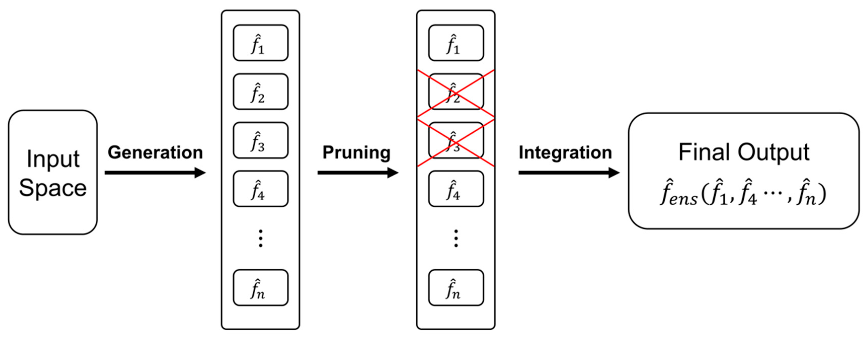
3.1. Ensemble Learning and ELQ: A Brief Review

Ensemble learning indicates a series of procedures to train several functions and combine their results based on an integrating rule [36]. Typically, the ensemble process consists of two parts: Ensemble generation and ensemble integration [37]. Some studies [38,39] added an ensemble pruning between the ensemble generation and integration. As it can be seen in Figure 2, in the first step (ensemble generation), a number of candidate functions (base learners) are generated. Then, the ensemble pruning step eliminates some of the generated functions in the first step. Finally, the ensemble integration combines the selected functions to reduce errors.

Kim et al. [14] introduced ELQ, which generates a more accurate estimate of Q by combining several functions obtained from several locations in river reaches. The generalized form of ELQ ($f_{ELQ}$) is:

$$f_{ELQ}=\alpha +w_1{\widehat{f}}_{i1}\left(X_{i1}\right)+w_2{\widehat{f}}_{i2}\left(X_{i2}\right)+\cdots +w_j{\widehat{f}}_{ij}\left(X_{ij}\right)+{\epsilon }_i,$$

(1)

where $X_{ij}$ is the observation of the hydraulic variables, $w_j$ is the weight determined by the ELQ integration process, and ${\widehat{f}}_{ij}$ is the base learner. $i$ indicates the $i$-th observation, and $j$ denotes the $j$-th variable, which represents a location of the obtained variable. $\mathsf{\alpha }$ and ${\epsilon }_i$ are the intercept and error term of ELQ, respectively. ELQ has $j$ number of base learners, but it is appropriate to have two or three base learners to avoid overfitting [14,40].

Here, candidate ensemble functions indicate several rating curves. We used a depth AHG relationship between historical in-situ Q data and H variations. Time series of H were obtained at different VSs using Envisat and Jason-2 altimetry data.

3.2. Generating Base Learners

Base learners for ELQ, which can be obtained from an empirical relationship (i.e., a rating curve) between H and in-situ Q data, were generated. Time series of H obtained from Envisat and Jason-2 altimetry can be found in Figure 3 and Figure 4.

The aim of ensemble generation is to produce a set of base learners for an ensemble integration step. First, before generating the rating curves, the flood travel time in the LMRB should be investigated since different VSs, located upstream and downstream of the in-situ Q stations, were used to estimate Q. Based on previous studies [18,19], the maximum flow peaks in August/September at Phnom Penh while September/October is the month of maximum flow at Tan Chau and TSL. In-situ water levels from 2003 to 2006 at four locations (see Figure 5), Stung Treng (ST), Phnom Penh (PP), Tan Chau (TC), and TSL, were obtained from ADPC. Using these in-situ water level data, we checked the peak flood dates, and they occurred in the order of ST, PP, TC, and TSL as shown by the dashed red line in Figure 5. The reason why the peak flood in TSL occurs after that in TC located downstream of TSL is because of the role of TSL in the flow reversal of the flood. In other words, the filling of TSL occurs in August/September, and the draining of TSL starts in September/October [18]. The peak flood time interval from ST to PP (blue line in x-axis in Figure 5) is more or less unchanged from 2003 to 2006. However, the peak flood time intervals from PP to TC (red line in x-axis in Figure 5) and from TC to TSL are irregular during the same period. The discrepancies for peak flood time intervals during these periods are because the peak flood timing upstream of Phnom Penh depends on the peak flood timing on the mainstem of the Mekong River and local hydrological characteristics, such as rainfall intensities and contributions from tributaries [19]. Therefore, we conclude that there is not enough evidence to determine the specific range of flood travel time for the LMRB.

Second, it is required to estimate water depth ($d$) to establish the rating curves. Here, $d$ was estimated from the depth–discharge ($d$–$Q$) relationship ($d=c{Q}^s$), generated using altimetry-derived H as in [14]. For details about generating the $d$–$Q$ relationship, readers are referred to [14]; only a brief procedure to obtain $d$ is provided here. Note that $d$ can be obtained from the equation $d=H-H_{min}+d_{min}$, where $H_{min}$ is the minimum H during the altimetry observation period, and $d_{min}$ can be obtained by $H_{min}$ minus $e$ (the height from the reference ellipsoid to the bottom of a cross-sectional wetted area). For Steps (1)–(3), the information used was not absolute H but relative H.

• Step (1): Calculate relative water stages ($D$); subtract $H_{min}$ from interpolated H.
• Step (2): Obtain the coefficient of determination ($R^2$) using the $d$–$Q$ relationship with 0.1-m increments on $D$.
• Step (3): Find the optimum $d_{min}$, where $R^2$ of the $d$–$Q$ relationship is maximized.

During the low water season, the TSL’s $d$ is reported to be 0.5 to 0.8 m [18,19]. However, as shown in

Table 3. Estimated $d_{min}$ (given in m) at seven VSs using datasets from the three in-situ Q stations.

VS	Stung Treng	Kratie	Tan Chau
EnvP565A	9.7	6.3	0.6
EnvP021A	5.0	4.6	0.0
EnvP952	28.4	24.8	2.2
EnvP866	3.9	6.8	0.0
EnvP021B	0.8	0.3	0.0
EnvP565B	5.5	4.2	0.0
EnvP651	10.9	13.7	0.0

, our estimated $d_{min}$ in TSL, for example, at EnvP952, were 28.4, 24.8, and 2.2 m with in-situ Q from Stung Treng, Kratie, and Tan Chau, respectively. The estimated $d_{min}$ at other VSs also showed different values. This shows that different $d_{min}$ at a VS were obtained using in-situ Q from different stations. Therefore, the optimal $d_{min}$ obtained from Steps (1)–(3) above cannot represent the real $d$ at that VS. Therefore, hereafter, $d$ is replaced by $d_V$, which indicates the obtained stage value from Steps (1)–(3). Note that the $d_V$–$Q$ relationship can still be effectively used as the base learner as shown in Figure 6 ($R^2$ > 0.70).

Third, in order to estimate daily Q, H were linearly interpolated. As shown in Figure 3, H showed a strong pattern of seasonality for all seven VSs, and therefore it is reasonable to use the daily interpolated H for base learners. Moreover, Kim et al. [17] demonstrated that degradation of the performance estimating Q due to the use of interpolated H can be mitigated with temporally denser acquisition of the original H by integrating more than two base learners. As previously mentioned, it was assumed that the in-situ Q stations were decommissioned after 31 December 2006. In order to train and validate the base learners, the linearly interpolated daily H were divided into training (1 January 2003 to 31 December 2005) and validation (1 January 2006 to 31 December 2006) datasets.

Finally, we obtained base learners using the power law relationship between $d_V$ and in-situ Q, such as:

$${\widehat{f}}_{ij}={\left(\frac{{(d_V)}_i}{c_j}\right)}^{1/s_j},$$

(2)

where $i$ indicates the $i$-th observation, $j$ denotes the virtual stations, $c_j$ and $s_j$ are the coefficients in the power law relationship ($d_V=c{Q}^s$), $d_V$ is the stage value estimated with specific in-situ Q data, and ${\widehat{f}}_{ij}$ is the generated base learner. Using the training dataset, unknown parameters $c_j$ and $s_j$ can be estimated.

3.3. Integrating Base Learners

After generating base learners, the final ensemble function can be obtained by a weighted average method [14]. Here, only two base learners were used for the final ensemble function since a large number of base learners may lead to overfitting [40]:

$$f_{ELQ}=\alpha ·1+w_1·{\widehat{f}}_{i1}+w_2·{\widehat{f}}_{i2}+{\epsilon }_i,$$

(3)

where $f_{ELQ}$ is the final ensemble function, ${\widehat{f}}_{i1}$ and ${\widehat{f}}_{i2}$ are base learners (generated ensemble functions), $w_1$ and $w_2$ are the weights of ELQ, $\alpha$ and ${\epsilon }_i$ are the intercept and error terms of ELQ, respectively, and $i$ indicates the $i$-th observation ($i$ = 1, 2, $\cdots$, $n$).

Ensemble pruning can also be performed before the integration process. Zhou [41] claimed that in order to obtain the best result in the ensemble process, the base learners that are less accurate should be excluded.

Table 4. $R^2$ of base learners at seven Envisat VSs with three different in-situ Q datasets.

VS	Stung Treng	Kratie	Tan Chau
EnvP565A	0.81	0.79	0.88
EnvP021A	0.93	0.90	0.83
EnvP952	0.46	0.47	0.80
EnvP866	0.95	0.93	0.80
EnvP021B	0.93	0.90	0.74
EnvP565B	0.80	0.80	0.69
EnvP651	0.88	0.87	0.76

shows $R^2$ of the base learners at seven Envisat VSs with in-situ Q datasets from three different stations. As can be seen from Figure 6, that shows box plots of those $R^{2}s$; outliers beyond the upper and lower whiskers were detected. The whisker values were set to half of the interquantile range (IQR), which corresponds to approximately $\pm$1.35$\sigma$ (where $\sigma$ is the standard deviation) and 82.3% coverage of the normally distributed data [42]. Based on this analysis, we decided to prune less accurate base learners in the ensemble integration process. Therefore, EnvP952 and EnvP565B were excluded for Q estimation at Stung Treng and Kratie and at Tan Chau, respectively.

3.4. Combining Multiple Radar Altimetry Missions

Although ELQ needs in-situ Q data to establish the rating curves and to obtain weights of the base learners, it can be used to fill missing Q data for decommissioned stream gauges. In other words, the discontinued Q data can be more accurately estimated using available historical in-situ Q data and the ELQ method. As previously mentioned, Bogning et al. [26] used several altimetry missions, such as ERS-2, Envisat, Satellite with Argos and AltiKa (SARAL/AltiKa), Cryosat-2, and Sentinel-3A, to estimate Q at Lambaréné in the Ogooué River Basin in Gabon, Central Africa, but the locations for estimating Q had to be close to VSs (e.g., within a few tens of kilometers). Therefore, the study did not use Jason-2 data, whose cross-track interval is about 315 km at the equator. On the contrary, we used several H obtained from Envisat and Jason-2 altimetry regardless of distances from in-situ Q stations since the ELQ method compensates degradation of performance for Q estimation due to a poor rating curve with VSs away from in-situ Q stations.

As shown in Table 1, in-situ Q data at Tan Chau is available only from 2003 to 2006 and from 2013 and 2016. Therefore, firstly, the training of base learners can be performed using historical in-situ Q data and Envisat-derived H from January 2003 to December 2005. Then, the trained ELQ can be validated using the validation dataset from January 2006 to December 2006.

Secondly, the trained ELQ can reconstruct Q for the ungauged period (test period) from January 2007 to October 2010. However, since the Envisat satellite moved to a new orbit on October 22 2010, the trained ELQ cannot be used to reconstruct Q after that date. Therefore, it is required to use other radar altimetry data; in this case, the Jason-2 altimeter. In contrast to a previous study [26] adopting multi-mission radar altimetry data with a single rating curve, consideration of inter-mission biases is not required in this study. In other words, rating curves generated from different altimetry missions in [26] should consider the inter-mission biases because locations for estimating Q had to be close to VSs, and locations of VSs from several altimetry missions are not generally matched. On the other hand, since ELQ obtains a relationship between H variations at several different VSs and historical Q data at a specific station, ELQ does not need to consider inter-mission biases. In other words, several rating curves for the ELQ process with multi-mission altimetry data can be obtained not at a single location, but at several different distant locations. In addition, owing to the overlapping period between Envisat and Jason-2 altimetry missions, the training step for Jason-2 was separated from the one for Envisat. Therefore, it is not required to consider inter-biases in this study.

Finally, Q data from October 2010 to 2016 can be estimated using ELQ with Jason-2-derived H. In this step, ELQ-estimated Q, which were reconstructed using the Envisat data from September 2008 to October 2010 (green box in Figure 7), can be used instead of in-situ Q data for the Jason-2 training step of ELQ. Since the $R^{2}s$ values of the base learners with J001L for Stung Treng and Kratie were 0.46 and 0.52, respectively (see

Table 5. $R^{2}s$ of base learners at four Jason-2 VSs with three different in-situ Q datasets.

VS	Stung Treng	Kratie	Tan Chau
J001L	0.46	0.52	0.84
J001U	0.93	0.93	0.71
J140	0.77	0.80	0.91
J179	0.93	0.91	0.68

), these weak base learners were pruned in the integration step. Using the obtained ELQ parameters in the Jason-2 training period, ELQ can now be used to estimate Q from October 2010 to September 2016, which includes the ungauged period, without the aid of in-situ Q data.

3.5. Performance Comparison

We compared ELQ-estimated Q (hereafter ${\widehat{Q}}_{ELQ}$) with estimates of Q obtained from a single rating curve, which is Model 1: $M_1=a_1·{\left(H-H_{min}\right)}^{\frac{5}{3}}+b_1$ (hereafter ${\widehat{Q}}_{M1}$) [5]. $a_1$ and $b_1$ are parameters to be calibrated with in-situ Q data.

Four metrics were adopted to evaluate the performance, including the mean error (ME), root mean square error (RMSE), relative RMSE (RRMSE), and Nash–Sutcliffe coefficient (NSE) [43,44], for ${\widehat{Q}}_{M1}$ and ${\widehat{Q}}_{ELQ}$. NSE ranges from $-\infty$ to 1, where 1 is the perfect match between the estimated and measured Q:

$$ME=\frac{{\sum }_{i=1}^n\left({\widehat{Q}}_i-Q_i\right)}{n·m_Q}\times 100 (\%),$$

(4)

$$RRMSE=\frac{RMSE}{m_Q}\times 100 (\%),$$

(5)

$$NSE=1-\frac{{\sum }_{i=1}^n{\left(Q_i-{\widehat{Q}}_i\right)}^2}{{\sum }_{i=1}^n{\left(Q_i-m_Q\right)}^2},$$

(6)

where $Q_i$ is the measured river discharge, $m_Q$ is the mean value of $Q_i$, ${\widehat{Q}}_i$ is the estimated river discharge, and $n$ is the number of observations.

4. Results

4.1. Estimating River Discharge Using Envisat-Derived Water Levels

Table 6. Comparison of ${\widehat{Q}}_{ELQ}$ and ${\widehat{Q}}_{M1}$ with in-situ Q at Stung Treng, Kratie, and Tan Chau in terms of mean error (ME) (%), root mean square error (RMSE) (m³s⁻¹), relative RMSE (RRMSE) (%), and Nash-Sutcliffe coefficient (NSE). Statistics from the training and validation datasets are separated by slashes.

Stung Treng	Used VS	ME (%)	RMSE (m3s−1)	RRMSE (%)	NSE
${\widehat{Q}}_{ELQ}$ (Best)	EnvP565A, 021B	0/-1.84	3441/3341	26.52/26.79	0.94/0.92
${\widehat{Q}}_{M1}$ (Best)	EnvP021B	0/-0.85	4222/3336	32.54/26.75	0.90/0.93
${\widehat{Q}}_{ELQ}$ (Worst)	EnvP565B, 651	0/-16.69	5577/5265	42.99/42.23	0.83/0.81
${\widehat{Q}}_{M1}$ (Worst)	EnvP565B	0/26.43	6214/6614	47.89/53.04	0.79/0.70
${\widehat{Q}}_{ELQ}$ (Average)	-	0/4.21	4071/4447	31.38/35.67	0.90/0.86
${\widehat{Q}}_{M1}$ (Average)	-	0/0.30	5234/4747	40.34/38.07	0.84/0.84
Kratie	Used VS	ME (%)	RMSE (m3s−1)	RRMSE (%)	NSE
${\widehat{Q}}_{ELQ}$ (Best)	EnvP021A, 565B	0/-5.43	4116/4077	28.88/27.10	0.91/0.92
${\widehat{Q}}_{M1}$ (Best)	EnvP866	0/2.20	4373/4896	30.69/32.55	0.90/0.88
${\widehat{Q}}_{ELQ}$ (Worst)	EnvP565B, 651	0/-22.82	5716/7366	40.11/48.97	0.84/0.73
${\widehat{Q}}_{M1}$ (Worst)	EnvP565B	0/-31.58	6361/8935	44.63/59.40	0.80/0.60
${\widehat{Q}}_{ELQ}$ (Average)	-	0/-5.54	4511/5219	31.65/34.70	0.90/0.86
${\widehat{Q}}_{M1}$ (Average)	-	0/-8.51	5593/5840	39.24/38.83	0.84/0.82
Tan Chau	Used VS	ME (%)	RMSE (m3s−1)	RRMSE (%)	NSE
${\widehat{Q}}_{ELQ}$ (Best)	EnvP866, 952	0/-2.95	1075/1304	11.72/12.97	0.97/0.96
${\widehat{Q}}_{M1}$ (Best)	EnvP565A	0/-12.38	2579/2642	28.11/26.27	0.84/0.83
${\widehat{Q}}_{ELQ}$ (Worst)	EnvP021B, 651	0/-12.26	3087/3571	33.65/35.51	0.77/0.70
${\widehat{Q}}_{M1}$ (Worst)	EnvP021B	0/-11.26	3812/3700	41.56/36.79	0.65/0.68
${\widehat{Q}}_{ELQ}$ (Average)	-	0/-6.82	2109/2206	22.99/21.93	0.88/0.87
${\widehat{Q}}_{M1}$ (Average)	-	0/-6.85	3182/3305	34.69/32.86	0.75/0.74

summarizes the performance of ${\widehat{Q}}_{M1}$ and ${\widehat{Q}}_{ELQ}$ for the three in-situ Q stations (Stung Treng, Kratie, and Tan Chau) according to the four metrics described in Section 3.4. In general, ${\widehat{Q}}_{ELQ}$ outperformed ${\widehat{Q}}_{M1}$ with both the training and validation datasets for all three in-situ Q stations. ${\widehat{Q}}_{ELQ}$ had overall RMSEs of 4071, 4511, and 2109 m³s⁻¹ (RRMSEs of 31.38%, 31.65%, and 22.99%) and NSEs of 0.90, 0.90, and 0.88 with the training dataset at Stung Treng, Kratie, and Tan Chau, respectively. On the other hand, ${\widehat{Q}}_{M1}$ had overall RMSEs of 5234, 5593, and 3182 m³s⁻¹ (RRMSEs of 40.34%, 39.24%, and 34.69%) and NSEs of 0.84, 0.84, and 0.75. The performances of ${\widehat{Q}}_{ELQ}$ and ${\widehat{Q}}_{M1}$ with the validation dataset were similar to those with the training dataset.

For Stung Treng, Kratie, and Tan Chau, the best results obtained from the training and validation datasets were ${\widehat{Q}}_{ELQ}$ from the combinations EnvP565A–021B, EnvP021A–565B, and EnvP866–952, respectively. However, there exists a possibility that the VS combination of the best ${\widehat{Q}}_{ELQ}$ from the test dataset (January 2007 to October 2010) might be different from that of the training and validation datasets due to different patterns in the variation of H in the training/validation and test datasets [45]. Since we used the parameters of ELQ obtained from the training dataset, it is advantageous to use the test dataset with a similar pattern to the training dataset. Additionally, the correlation coefficient ($r$) between two base learners (${\widehat{f}}_{i1}$ and ${\widehat{f}}_{i2}$) should be small in order to maximize the performance of ELQ [14]. To analyze the best combination of VSs for the test dataset, a comparison of $r$ obtained from Envisat-derived H between the training and test datasets was performed as shown in Figure 8. For Stung Treng, the best base learner was obtained from EnvP021B (see Table 6). In order to select the best combination with EnvP021B, $r$ should be small as much as possible in both the training and test datasets. Since $r$ obtained from H between EnvP565A and EnvP021B was the smallest, the combination EnvP565A–021B was selected for the test dataset for ELQ. Similarly, the combinations EnvP866–EnvP565A and EnvP866–EnvP952 were selected for the test dataset of ELQ for Kratie (Figure 8b) and Tan Chau (Figure 8c), respectively.

Table 7. Comparison of ${\widehat{Q}}_{ELQ}$ and ${\widehat{Q}}_{M1}$ with in-situ Q at Stung Treng, Kratie, and Tan Chau in terms of ME (%), RMSE (m³s⁻¹), RRMSE (%), and NSE using the test dataset.

Stung Treng	Used VS	ME (%)	RMSE (m3s−1)	RRMSE (%)	NSE
${\widehat{Q}}_{ELQ}$	EnvP565A, 021B	–1.64	3737	31.78	0.88
${\widehat{Q}}_{M1}$	EnvP021B	–3.29	5142	43.73	0.78
Kratie	Used VS	ME (%)	RMSE (m3s−1)	RRMSE (%)	NSE
${\widehat{Q}}_{ELQ}$	EnvP565A, 866	9.38	4058	32.43	0.88
${\widehat{Q}}_{M1}$	EnvP866	12.12	5072	40.53	0.82
Tan Chau	Used VS	ME (%)	RMSE (m3s−1)	RRMSE (%)	NSE
${\widehat{Q}}_{ELQ}$	EnvP866, 952	0.61	1727	19.03	0.91
${\widehat{Q}}_{M1}$	EnvP565A	–3.41	2328	25.65	0.83

compares the performance of ${\widehat{Q}}_{M1}$ and ${\widehat{Q}}_{ELQ}$ for the three in-situ Q stations according to the four metrics with the test dataset. Similar to the results from the training and validation datasets, ${\widehat{Q}}_{ELQ}$ outperformed ${\widehat{Q}}_{M1}$ for all three locations. It should be noted that in-situ water levels at Tan Chau were used for generating pseudo-in-situ Q for statistics in Table 6 since in-situ Q at Tan Chau does not exist for the test period. Hydrographs for the training and validation datasets are shown in Figure 9. In the case of Stung Treng and Kratie, ${\widehat{Q}}_{M1}$ and ${\widehat{Q}}_{ELQ}$ showed a similar pattern. However, ${\widehat{Q}}_{M1}$ were inaccurate in the high-water season of 2009. These inaccurate ${\widehat{Q}}_{M1}$ might be attributed to the test dataset, which has a different H pattern compared to the training dataset [46]. In other words, the fluctuating Q pattern in the high-water season of 2009 might affect the performance of ${\widehat{Q}}_{M1}$ whereas ${\widehat{Q}}_{ELQ}$ showed a better fit to in-situ Q because ELQ combines two base learners. In the case of Tan Chau, ${\widehat{Q}}_{ELQ}$ outperformed ${\widehat{Q}}_{M1}$ since the pattern of Q at Tan Chau is affected by TSL and the Mekong mainstem [18].

4.2. Estimating River Discharge Using Jason-2-Derived Water Levels

Once ${\widehat{Q}}_{ELQ}$ from January 2007 to October 2010 with Envisat-derived H are obtained, we can train the base learners with Jason-derived H and ${\widehat{Q}}_{ELQ}$ in the overlapping period from September 2008 to October 2010. The ensemble generation and integration with the four Jason-derived H were performed for the overlap period. After obtaining base learners with Jason-derived H, ${\widehat{Q}}_{ELQ}$ were estimated from October 2010 to September 2016.

Table 8. Comparison of ${\widehat{Q}}_{ELQ}$ and ${\widehat{Q}}_{M1}$ with respect to in-situ Q at Stung Treng, Kratie, and Tan Chau using Jason-derived H. Statistics from the training and validation datasets are separated by slashes.

Stung Treng	Used VS	ME (%)	RMSE (m3s−1)	RRMSE (%)	NSE	r
${\widehat{Q}}_{ELQ}$ (Best)	J001U, 179	0.41/2.33	3752/2915	31.62/22.31	0.88/0.94	0.95/0.95
${\widehat{Q}}_{ELQ}$	J140,179	0.41/10.58	3779/3343	31.84/25.59	0.87/0.92	0.79/0.75
${\widehat{Q}}_{M1}$ (Best)	J001U	0.41/0.65	3354/2848	28.27/21.80	0.90/0.94	-
${\widehat{Q}}_{M1}$	J140	0.41/16.80	5501/6980	46.36/53.42	0.73/0.66	-
${\widehat{Q}}_{M1}$	J179	0.41/2.84	4847/3926	40.84/30.05	0.79/0.89	-
Kratie	Used VS	ME (%)	RMSE (m3s−1)	RRMSE (%)	NSE	r
${\widehat{Q}}_{ELQ}$	J001U, 179	14.15/18.00	4788/5443	39.69/46.15	0.82/0.79	0.95/0.95
${\widehat{Q}}_{ELQ}$ (Best)	J140,179	14.15/21.54	4497/5157	37.28/43.73	0.84/0.81	0.79/0.75
${\widehat{Q}}_{M1}$ (Best)	J001U	14.15/19.03	4501/7281	37.31/61.74	0.84/0.62	-
${\widehat{Q}}_{M1}$	J140	14.15/26.25	5797/7202	48.05/61.07	0.73/0.63	-
${\widehat{Q}}_{M1}$	J179	14.15/15.54	5840/6084	48.41/51.59	0.73/0.73	-
Tan Chau	Used VS	ME (%)	RMSE (m3s−1)	RRMSE (%)	NSE	r
${\widehat{Q}}_{ELQ}$ (Best)	J001L, 179	–0.99/–7.66	1529/2045	16.10/21.64	0.93/0.89	0.56/0.60
${\widehat{Q}}_{ELQ}$	J140,179	–0.99/5.52	2536/3103	26.70/32.83	0.80/0.75	0.79/0.75
${\widehat{Q}}_{M1}$ (Best)	J001L	–0.99/–10.15	1826/3066	19.23/32.43	0.90/0.75	-
${\widehat{Q}}_{M1}$	J140	–0.99/6.16	2409/3311	25.37/35.02	0.82/0.71	-
${\widehat{Q}}_{M1}$	J179	–0.99/–1.23	4232/4064	44.57/42.99	0.45/0.57	-

compares the performance of ${\widehat{Q}}_{M1}$ and ${\widehat{Q}}_{ELQ}$ for the three in-situ Q stations. In contrast to the experiment with Envisat-derived H, the performance difference between ${\widehat{Q}}_{M1}$ and ${\widehat{Q}}_{ELQ}$ was marginal for Stung Treng and Kratie. The performance of ${\widehat{Q}}_{M1}$ was actually slightly better than ${\widehat{Q}}_{ELQ}$ at Stung Treng. The reason for this relatively poor performance for ${\widehat{Q}}_{ELQ}$ is likely due to the lack of base learners’ diversity [41,47]; as $r$ increases, the diversity of base learners decreases. On the other hand, as can be seen in Table 8, if we consider only J140 and J179 for the ELQ process, the performance of ${\widehat{Q}}_{ELQ}$ was better than that of ${\widehat{Q}}_{M1}$ due to enhanced diversity (i.e., smaller $r$). Similarly, ${\widehat{Q}}_{ELQ}$ with the combination J001L–J179 ($r$ < 0.60) showed better performance than ${\widehat{Q}}_{M1}$ with both the training and validation datasets for Tan Chau. Hydrographs of Jason-derived ${\widehat{Q}}_{M1}$ and ${\widehat{Q}}_{ELQ}$ are shown in Figure 10. Note that hydrographs for Stung Treng were generated until December 2012 due to the availability of in-situ Q data. Due to the relatively simple pattern of Q from Stung Treng, hydrographs of ${\widehat{Q}}_{M1}$ and ${\widehat{Q}}_{ELQ}$ were similar. On the other hand, due to a more complex pattern of Q at Kratie, ${\widehat{Q}}_{ELQ}$ showed a better fit to in-situ Q in the validation period (see Table 8 and Figure 11). In the case of Tan Chau, in general, ${\widehat{Q}}_{ELQ}$ agreed better with in-situ Q than ${\widehat{Q}}_{M1}$.

5. Discussions

5.1. Analysis of ELQ’s Performance

In this section, the performance of ELQ was analyzed by three indices, degree of compensation ($I_{DoC}$) [14], degree of dominance ($I_{DoD}$) [48], and power of base learner ($P_{BL}$) [17]. The analyses were performed with Envisat-derived ${\widehat{Q}}_{ELQ}$ since the available number of combinations with Jason-derived ${\widehat{Q}}_{ELQ}$ was small (i.e., <4).

Firstly, it was found that a lower $r$ between two VSs can provide better estimates of Q in the ELQ process. Kim et al. [14] introduced the performance index of ELQ, $I_{DoC}$:

$$I_{DoC}=\left(1-r_{mn}\right),$$

(7)

where $mn$ is the combination pairs of the variables, and $r$ is the correlation coefficient between variables in the combination pairs. $I_{DoC}$ ranges from 0 (no compensation) to 1 (perfect compensation). As shown in Figure 11a–c, Q improvements increased when $I_{DoC}$ increased, where Q improvement (m³s⁻¹) is defined as RMSE difference between ${\widehat{Q}}_{M1}$ and ${\widehat{Q}}_{ELQ}$:

$$Qimprovement=RMSE\left({\widehat{Q}}_{M1}\right)-RMSE\left({\widehat{Q}}_{ELQ}\right).$$

(8)

Secondly, Kim et al. [48] developed a performance index for ELQ termed $I_{DoD}$:

$$I_{DoD}=w_{max}-w_{min},$$

(9)

where $w_{max}$ and $w_{min}$ are the maximum and minimum weights. Note that the sum of weights ($w_{max}$ + $w_{min}$) is 1. $I_{DoD}$ ranges from 0 (uniformly distributed dominance) to 1 (skewed dominance). Since the weights ($w_{max}$ and $w_{min}$) are assigned in the weighted average method, these weights are determined by the importance of the respective base learner. The study in [17] analyzed the relationship between $I_{DoD}$ and Q improvement over the central Congo River. They found that Q improvement increases when $I_{DoD}$ decreases ($R^2$ = 0.74). This relationship is also confirmed in this study (Figure 11d–f); $R^{2}s$ between $I_{DoD}$ and Q improvement from Stung Treng, Kratie, and Tan Chau were 0.48, 0.46, and 0.47, respectively. In some cases, the value of the weight is biased toward one variable because $r$ between the two variables is strongly correlated (e.g., $I_{DoC}$ < 0.10) [49]. The biased weight implies that the additional base learner, which has a smaller weight, has limited additional information. Consequently, the performance of ${\widehat{Q}}_{ELQ}$ becomes comparable to that of traditional methods using ${\widehat{Q}}_{M1}$.

Thirdly, Kim et al. [17] also introduced another performance index for ELQ termed power of base learner ($P_{BL}$), which is calculated by averaging the NSEs of base learners. In order to investigate the relationship with Q improvement, $P_{BL}$, and $I_{DoC}$, each result was color-coded with $I_{DoC}$, as shown in Figure 11g–i. In contrast to the results in [17], which showed a positive relationship between Q improvement and $P_{BL}$, these two showed a negative relationship for Stung Treng, Kratie, and Tan Chau. The reason for this negative relationship is likely due to a greater $P_{BL}$ from the LMRB. In other words, although more base learners were added in the ELQ process, no improvement in Q estimation was made when the performance of each base learner was high enough (e.g., NSE > 0.90). On the other hand, the values with higher Q improvement (e.g., reddish dots in Figure 11i) showed relatively low $P_{BL}$. This demonstrates that Q improvement becomes maximized when relatively weak base learners are integrated [40].

5.2. Parsimonious Model of ELQ

In this study, only two base learners were used for ELQ. As described in [14], a large number of base learners can lead to overfitting, and therefore, it is necessary to determine the optimal number of base learners. Similar to [14], we investigated the performance of ELQ using two to six base learners with Envisat-derived H for Tan Chau as an example. As shown in

Table 9. An example of the performance metrics obtained from the training and validation datasets with Envisat-derived H for Tan Chau. Statistics from the training and validation datasets are separated by slashes.

Number of VSs Used	Passes of the Added VSs	ME (%)	RMSE (m3s−1)	RRMSE (%)	NSE	Number of Effective Weights
2	EnvP866,952	0/–2.95	1075/1304	11.72/12.97	0.97/0.96	2
3	565A	0/–3.98	1032/1237	11.25/12.30	0.97/0.96	3
4	021A	0/–2.60	953/1270	10.38/12.62	0.98/0.96	3
5	021B	0/–4.26	885/1268	9.65/12.61	0.98/0.96	3
6	651A	0/–3.63	874/1307	9.52/12.99	0.98/0.96	3

, with more VSs, the performance metrics were slightly improved in the training dataset, but no significant improvement was made in the validation dataset. The number of effective weights remained at three. This indicates that more than three base learners made no additional contribution because the added base learners might be highly correlated with the existing base learners, or the NSE of the added base learner was worse than that of the existing ones. Therefore, it might be optimal to use three base learners. However, compared to the result obtained from two base learners, improvement in the performance of ELQ was negligible when three were used. Therefore, we decided to use only two base learners in this study (principle of parsimony) [50].

5.3. ELQ Versus AMHG?

The strength of the ELQ process is that it can combine several base learners, which are obtained from spatially distributed VSs. Using H obtained from several VSs for the estimation of Q is a new concept since a single rating curve has traditionally been generated for the estimation of Q at a specific location. On the other hand, Gleason and Smith [51] introduced a method estimating Q without the aid of in-situ Q using the so-called at-many-stations hydraulic geometry (AMHG), which uses log-linearly related parameters in AHG geometry ($W=a{Q}^b, d=c{Q}^s, v=k{Q}^m$, where $W$ = width, $d$ = depth, $v$ = velocity, $Q$ = discharge, and $a,b,c,s,k,m$ are empirical parameters). Among three log-linear relationships (i.e., $a$–$b$, $c$–$s$, and $k$–$m$), the $a$–$b$ relationship has mainly been selected for their studies since river widths along river reaches can be easily extracted from satellite images. The AMHG approach does not require in-situ Q data. However, the accuracy of Q estimation ranges with an RRMSE of 20% to 30% when compared with in-situ Q data [51]. Moreover, the AMHG uses a genetic algorithm (GA) to retrieve instantaneous Q for each observation date [51]. Therefore, this process might be computationally expensive compared to an empirical method. Additionally, since optical satellite images, such as Landsat Thematic Mapper imagery, were adopted to estimate Q using AMHG [51,52,53], estimating Q at a target location that is covered with clouds can be somewhat limited.

Both AMHG and ELQ use several AHG relationships generated from many stations, but they differ in the way they combine the AHG relationships. In order to investigate the similarity between the AMHG and ELQ, we tested the existence of the AMHG relationship at three locations, Stung Treng, Kratie, and Tan Chau with Envisat-derived H. As shown in Figure 12, the log-linear relationship between log $c$ and $s$ was consistent in all three locations. Our findings indicate that the AMHG formulation is conserved with H even along a relatively long river reach (~a few hundreds of kilometers) although Gleason and Smith [51] assumed that the log-linear relationships exist with many AHG pairs obtained from river reaches only within ~10 km.

The primary difference between AMHG and ELQ for the estimation of Q is that the AMHG focuses on the correlative relationship between coefficients and exponents among many AHG relationships, whereas ELQ concentrates on the difference among several AHG relationships, which cannot be identified in the log-linear relationship. In other words, AMHG estimates Q using shared information among many AHG relationships without the aid of in-situ Q while ELQ uses the identified complementary information from several AHG relationships in an ensemble learning process. Therefore, a synergy between AMHG and ELQ could be made based on the recent finding in [17], which obtained more accurate Q with an RRMSE of 7% to 10%, with ELQ and a hydrologic model-derived Q, whose daily accuracy was about RRMSE of 15% to 18%. Similarly, the accuracy of AMHG-derived Q could be further improved with ELQ.

6. Conclusions

This study demonstrated that more accurate daily Q estimates can be obtained with ELQ and multi-mission radar altimetry data over the LMRB from 2003 to 2016. In the case of Tan Chau, the RMSE of ${\widehat{Q}}_{ELQ}$ obtained from EnvP866 and EnvP952 decreased by 1504/1338 m³s⁻¹ with Envisat-derived H for the training/validation datasets. This corresponds to the mean annual Q of the Arkansas River (Arkansas, USA; 1128 m³s⁻¹), which is a major tributary of the Mississippi River. Once the ELQ model was established in the training period, ${\widehat{Q}}_{ELQ}$ were reconstructed with Envisat-derived H from January 2007 to October 2010. Then, Jason-derived H were trained using the reconstructed ${\widehat{Q}}_{ELQ}$ from September 2008 to October 2010. Finally, we estimated ${\widehat{Q}}_{ELQ}$ from October 2010 to September 2016 with Jason-derived H. Our results showed that ELQ can successfully estimate Q even if only a few VSs exist along a river reach. In other words, since the ELQ method compensates for degradation of the performance of Q estimation due to poor rating curves with the VSs away from in-situ Q stations, we could obtain improved Q estimates using ELQ and Jason-2 altimetry data compared to the estimates obtained from a single rating curve.

Our results are in alignment with [14,17], who concluded that (1) ELQ outperforms the previous method based on a single rating curve, (2) $I_{DoC}$ is one of the contributing factors determining the performance of ELQ, and (3) improvement of Q estimation might not be obtained when the performance of each base learner is high enough (e.g., NSE > 0.90).

In a future study, we will also use H from other altimetry missions, such as Sentinel-3A/B and Jason-3, in order to obtain a finer temporal resolution and enhance ELQ’s performance. We will also apply ELQ to several other poorly gauged river basins to expand our knowledge of Q variation globally.

References

1. Vörösmarty, C.J.; Green, P.; Salisbury, J.; Lammers, R.B. Global water resources: Vulnerability from climate change and population growth. Science 2000, 289, 284–288. [Google Scholar] [CrossRef] [PubMed]
2. Alsdorf, D.E.; Rodriguez, E.; Lettenmaier, D.P. Measuring surface water from space. Rev. Geophys. 2007, 45, 1–24. [Google Scholar] [CrossRef]
3. Shiklomanov, A.I.; Lammers, R.B.; Vörösmarty, C.J. Widespread decline in hydrological monitoring threatens pan-Arctic research. Eos Trans. 2002, 83, 13–17. [Google Scholar] [CrossRef]
4. Bjerklie, D.M.; Birkett, C.M.; Jones, J.W.; Carabajal, C.; Rover, J.A.; Fulton, J.W.; Garambois, P.A. Satellite remote sensing estimation of river discharge: Application to the Yukon River Alaska. J. Hydrol. 2018, 561, 1000–1018. [Google Scholar] [CrossRef]
5. Sichangi, A.W.; Wang, L.; Yang, K.; Chen, D.; Wang, Z.; Li, X.; Zhou, J.; Liu, W.; Kuria, D. Estimating continental river basin discharges using multiple remote sensing data sets. Remote Sens. Environ. 2016, 179, 36–53. [Google Scholar] [CrossRef]
6. Manning, R. On the flow of water in open channels and pipes. Inst. Civ. Eng. Irel. Trans. 1891, 20, 161–207. [Google Scholar]
7. Smith, L.C.; Pavelsky, T.M. Estimation of river discharge, propagation speed, and hydraulic geometry from space: Lena River, Siberia. Water Resour. Res. 2008, 44, W03427. [Google Scholar] [CrossRef]
8. Paris, A.; Dias de Paiva, R.; Santos da Silva, J.; Medeiros Moreira, D.; Calmant, S.; Garambois, P.A.; Collischonn, W.; Bonnet, M.P.; Seyler, F. Stage-discharge rating curves based on satellite altimetry and modeled discharge in the Amazon basin. Water Resour. Res. 2016, 52, 3787–3814. [Google Scholar] [CrossRef]
9. Leopold, L.B.; Maddock, T. The Hydraulic Geometry of Stream Channels and Some Physiographic Implications; U.S. Government Printing Office: Washington, DC, USA, 1953; Volume 252.
10. Richard, K.S. Complex width-discharge relations in natural river sections. Geol. Soc. Am. Bull. 1976, 87, 199–206. [Google Scholar] [CrossRef]
11. Phillips, J.D. The instability of hydraulic geometry. Water Resour. Res. 1990, 26, 739–744. [Google Scholar] [CrossRef]
12. Jowett, I.G. Hydraulic geometry of New Zealand rivers and its use as a preliminary method of habitat assessment. Regul. Rivers Res. Mgmt. 1998, 14, 451–466. [Google Scholar] [CrossRef]
13. Mersel, M.K.; Smith, L.C.; Andreadis, K.M.; Durand, M.T. Estimation of river depth from remotely sensed hydraulic relationships. Water Resour. Res. 2013, 49, 3165–3179. [Google Scholar] [CrossRef]
14. Kim, D.; Yu, H.; Beighley, E.; Durand, M.; Alsdorf, D.E. Ensemble learning regression for estimating river discharges using satellite altimetry data: Central Congo River as a test-bed. Remote Sens. Environ. 2019, 221, 741–755. [Google Scholar] [CrossRef]
15. Roux, E.; Cauhope, M.; Bonnet, M.P.; Calmant, S.; Vauchel, P.; Seyler, F. Daily water stage estimated from satellite altimetric data for large river basin monitoring. Hydrol. Sci. J. 2008, 53, 81–99. [Google Scholar] [CrossRef]
16. Kim, D.; Lee, H.; Laraque, A.; Tshimanga, R.M.; Yuan, T.; Jung, H.C.; Beighley, E.; Chang, C.H. Mapping spatio-temporal water level variations over the central Congo River using PALSAR ScanSAR and Envisat altimetry data. Int. J. Remote Sens. 2017, 38, 7021–7040. [Google Scholar] [CrossRef]
17. Kim, D.; Lee, H.; Beighley, E.; Tshimanga, R.M. Estimating discharges for poorly gauged river basin using ensemble learning regression with satellite altimetry data and a hydrologic model. Adv. Space Res. 2019, in press. [Google Scholar] [CrossRef]
18. Mekong River Commission. Overview of the Hydrology of the Mekong Basin; Mekong River Commission: Vientiane, Lao PDR, 2005; p. 82. [Google Scholar]
19. Kummu, M.; Sarkkula, J. Impact of the Mekong River flow alteration on the Tonle Sap flood pulse. AMBIO 2008, 37, 185–192. [Google Scholar] [CrossRef]
20. Pagano, T.C. Evaluation of Mekong River Commission operational flood forecasts, 2000–2012. Hydrol. Earth Syst. Sci. 2014, 18, 2645–2656. [Google Scholar] [CrossRef]
21. Chang, C.H.; Lee, H.; Hossain, F.; Basnayake, S.; Jayasinghe, S.; Chishtie, F.; Saah, D.; Yu, H.; Sothea, K.; Du Bui, D. A model-aided satellite-altiemtry-based flood forecasting system for the Mekong River. Environ. Model. Softw. 2019, 112, 112–127. [Google Scholar] [CrossRef]
22. Wang, W.; Lu, H.; Yang, D.; Sothea, K.; Jiao, Y.; Gao, B.; Peng, X.; Pang, Z. Modelling hydrologic processes in the Mekong River Basin using a distributed model driven by satellite precipitation and rain gauge observations. PLoS ONE 2016, 11, e0152229. [Google Scholar] [CrossRef]
23. Mohammed, I.N.; Bolten, J.D.; Srinivasa, R.; Lakshmi, V. Satellite observations and modeling to understand the Lower Mekong River Basin streamflow variability. J. Hydrol. 2018, 564, 559–573. [Google Scholar] [CrossRef]
24. Delgado, J.M.; Apel, H.; Merz, B. Flood trends and variability in the Mekong river. Hydrol. Earth Syst. Sci. 2010, 14, 407–418. [Google Scholar] [CrossRef]
25. Hossain, F.; Sikder, S.; Biswas, N.; Bonnema, M.; Lee, H.; Luong, N.D.; Hiep, N.H.; Du Duong, B.; Long, D. Predicting water availability of the regulated Mekong river basin using satellite observations and a physical model. Asian J. Water Environ. 2017, 14, 39–48. [Google Scholar] [CrossRef]
26. Bogning, S.; Frappart, F.; Blarel, F.; Niño, F.; Mahé, G.; Bricquet, J.P.; Seyler, F.; Onguéné, R.; Etamé, J.; Paiz, M.C.; et al. Monitoring water levels and discharges using radar altimetry in an ungauged river basin: The case of the Ogooué. Remote Sens. 2018, 10, 350. [Google Scholar] [CrossRef]
27. Birkinshaw, S.J.; Moore, P.; Kilsby, C.G.; O’donnell, G.M.; Hardy, A.J.; Berry, P.A.M. Daily discharge estimation at ungauged river sites using remote sensing. Hydrol. Process. 2014, 28, 1043–1054. [Google Scholar] [CrossRef]
28. Birkinshaw, S.J.; O’donnell, G.M.; Moore, P.; Kilsby, C.G.; Fowler, H.J.; Berry, P.A.M. Using satellite altimetry data to augment flow estimation techniques on the Mekong River. Hydrol. Process. 2010, 24, 3811–3825. [Google Scholar] [CrossRef]
29. Mohammed, I.N.; Bolten, J.D.; Srinivasan, R.; Meechaiya, C.; Spruce, J.P.; Lakshmi, V. Ground and satellite based observation datasets for the Lower Mekong River Basin. Data Brief. 2018, 21, 2020–2027. [Google Scholar] [CrossRef]
30. Frappart, F.; Calmant, S.; Cauhopé, M.; Seyler, F.; Cazenave, A. Preliminary results of ENVISAT RA-2-derived water levels validation over the Amazon basin. Remote Sens. Environ. 2006, 100, 252–264. [Google Scholar] [CrossRef]
31. Lee, H.; Shum, C.K.; Emery, W.; Calmant, S.; Deng, X.; Kuo, C.Y.; Roesler, C.; Yi, Y. Validation of Jason-2 altimeter data by waveform retracking over California coastal ocean. Mar. Geod. 2010, 33, 304–316. [Google Scholar] [CrossRef]
32. Fernandes, M.; Lázaro, C.; Nunes, A.; Scharroo, R. Atmospheric corrections for altimetry studies over inland water. Remote Sens. 2014, 6, 4952–4997. [Google Scholar] [CrossRef]
33. Siddique-E-Akbor, A.H.M.; Hossain, F.; Lee, H.; Shum, C.K. Inter-comparison study of water level estimates derived from hydrodynamic–hydrologic model and satellite altimetry for a complex deltaic environment. Remote Sens. Environ. 2011, 115, 1522–1531. [Google Scholar] [CrossRef]
34. Okeowo, M.A.; Lee, H.; Hossain, F.; Getirana, A. Automated generation of lakes and reservoirs water elevation changes from satellite radar altimetry. IEEE J. STARS 2017, 10, 3465–3481. [Google Scholar] [CrossRef]
35. Schwatke, C.; Dettmering, D.; Bosch, W.; Seitz, F. DAHITI—An innovative approach for estimating water level time series over inland waters using multi-mission satellite altimetry. Hydrol. Earth Syst. Sci. 2015, 19, 4345–4364. [Google Scholar] [CrossRef] [Green Version]
36. Brown, G. Ensemble learning. In Encyclopedia of Machine Learning; Sammut, C., Webb, G.I., Eds.; Springer: Boston, MA, USA, 2011; pp. 312–320. [Google Scholar]
37. Zhou, Z.H. Ensemble learning. In Encyclopedia of Biometrics; Li, S.Z., Jain, A., Eds.; Springer: Boston, MA, USA, 2015; pp. 411–416. [Google Scholar]
38. Mendes-Moreira, J.; Soares, C.; Jorge, A.M.; Sousa, J.F.D. Ensemble approaches for regression: A survey. ACM Comput. Surv. 2012, 45, 10. [Google Scholar] [CrossRef]
39. Roli, F.; Giacinto, G.; Vernazza, G. Methods for designing multiple classifier systems. In International Workshop on Multiple Classifier Systems; Springer: Berlin, Germany, 2001; pp. 78–87. [Google Scholar]
40. Schapire, R.E.; Freund, Y. Boosting: Foundations and algorithms. In Adaptive Computation and Machine Learning Series; Dietterich, T., Ed.; MIT Press: London, UK, 2012; pp. 1–527. [Google Scholar]
41. Zhou, Z.H. Ensemble learning. In Encyclopedia of Database Systems; Liu, L., Özsu, M.T., Eds.; Springer: Boston, MA, USA, 2009; pp. 988–991. [Google Scholar]
42. Krzywinski, M.; Altman, N. Visualizing samples with box plots. Nat. Methods 2014, 11, 119–120. [Google Scholar] [CrossRef]
43. Nash, J.E.; Sutcliffe, J.V. River flow forecasting through conceptual models part I–A discussion of principles. J. Hydrol. 1970, 10, 282–290. [Google Scholar] [CrossRef]
44. Dingman, S.L. Statistical concepts useful in hydrology. In Physical Hydrology, 2nd ed.; Dingman, S.L., Ed.; Waveland Press, Inc.: Long Grove, IL, USA, 2002; pp. 552–581. [Google Scholar]
45. Murphy, K.P. Introduction. In Machine Learning: A Probabilistic Perspective; Murphy, K.P., Ed.; MIT Press: London, UK, 2014; pp. 1–26. [Google Scholar]
46. Dietterich, T.G. Machine-learning research. AI Mag. 1997, 18, 97. [Google Scholar]
47. Brown, G.; Wyatt, J.; Harris, R.; Yao, X. Diversity creation methods: A survey and categorisation. Inf. Fusion 2005, 6, 5–20. [Google Scholar] [CrossRef]
48. Kim, D.; Lee, H.; Yu, H.; Jayasinghe, S.; Basnayake, S.B.; Chishtie, F.; Bui, D.D.; Nguyen, L.D.; Hwang, E. Deriving Daily Discharges from Satellite Radar Altimetry and Ensemble Learning Regression in Poorly Gauged River Basins. In Proceedings of the AGU Fall Meeting, Washington, DC, USA, 10–14 December 2018. Abstract Number GC31K–1384. [Google Scholar]
49. Breiman, L. Stacked regressions. Mach. Learn. 1996, 24, 49–64. [Google Scholar] [CrossRef] [Green Version]
50. Schuenemeyer, J.H.; Drew, L.J. Modeling Concepts. In Statistics for Earth and Environmental Scientists; Schuenemeyer, J.H., Drew, L.J., Eds.; John Wiley & Sons: Hoboken, NJ, USA, 2011; pp. 37–50. [Google Scholar]
51. Gleason, C.J.; Smith, L.C. Toward global mapping of river discharge using satellite images and at-many-stations hydraulic geometry. Proc. Natl. Acad. Sci. USA 2014, 111, 4788–4791. [Google Scholar] [CrossRef] [Green Version]
52. Gleason, C.J.; Smith, L.C.; Lee, J. Retrieval of river discharge solely from satellite imagery and at-many-stations hydraulic geometry: Sensitivity to river form and optimization parameters. Water Resour. Res. 2014, 50, 9604–9619. [Google Scholar] [CrossRef]
53. Gleason, C.J.; Wang, J. Theoretical basis for at-many-stations hydraulic geometry. Geophys. Res. Lett. 2015, 42, 7107–7114. [Google Scholar] [CrossRef] [Green Version]
Figure 1. Map of the Lower Mekong River. The yellow and red lines indicate ground tracks of Envisat and Jason-2 altimetry, respectively. The white triangles indicate the in-situ gauges at Tan Chau, Kratie, and Stung Treng. The green triangles represent virtual stations. The white square is the reference location at Phnom Penh. (map data ©2019 Google).
Remotesensing 11 02684 g001
Figure 2. Conceptual design of the ensemble learning process (modified from Figure 2 in [14]). f ^ i are the candidate functions ( i = 1, 2, , n ) generated in the ensemble generation process, and f ^ e n s is the final ensemble model combining { f ^ 1 , f ^ 4 , , f ^ n } after pruning several functions (i.e., f ^ 2 and f ^ 3 ).
Remotesensing 11 02684 g002
Figure 3. Envisat-derived water levels at seven virtual stations from 2002 to 2010.
Remotesensing 11 02684 g003
Figure 4. Jason-2-derived water levels at four virtual stations from 2008 to 2016.
Remotesensing 11 02684 g004
Figure 5. Time series plots of water levels from four in-situ stations in (a) 2003, (b) 2004, (c) 2005, and (d) 2006. The blue, purple, green, and black lines indicate water levels at Stung Treng (ST), Phnom Penh (PP), Tan Chau (TC), and Tonle Sap Lake (TSL), respectively. The red dots represent the peak flood dates whose ranges are August–September for ST and PP, and September–October for TC and TSL. The cross marks in the x-axis were added for visualization of the intervals of peak flood timing among the four stations.
Remotesensing 11 02684 g005
Figure 6. Box plots of R 2 of base learners at seven Envisat VSs with the three different in-situ Q datasets. The red crosses indicate outliers that are beyond the upper and lower whisker values.
Remotesensing 11 02684 g006
Figure 7. Schematic illustration of combining multiple radar altimetry missions from 2002 to 2017 (satellite figures©2019 European Space Agency). Note that the orange bars indicate the availability of in-situ Q data at Tan Chau.
Remotesensing 11 02684 g007
Figure 8. Comparison of correlation coefficients for Envisat-derived H between training dataset (January 2003 to December 2005) and test dataset (January 2007 to October 2010) for (a) Stung Treng, (b) Kratie, and (c) Tan Chau.
Remotesensing 11 02684 g008
Figure 9. Comparison among in-situ Q (blue), Q ^ M 1 (green), and Q ^ E L Q (red) for (a) Stung Treng, (b) Kratie, and (c) Tan Chau. Q ^ E L Q data from the test datasets were obtained from the combinations EnvP565A–021B (Stung Treng), EnvP565A–866 (Kratie), and EnvP866–952 (Tan Chau) (see Table 7). Q ^ M 1 data from the test datasets were obtained from EnvP021B (Stung Treng), EnvP866 (Kratie), and EnvP565A (Tan Chau). The blue vertical lines were added for visual clarity among training, validation, and test datasets.
Remotesensing 11 02684 g009
Figure 10. Comparison among in-situ Q (blue), Q ^ M 1 (green), and Q ^ E L Q (red) for (a) Stung Treng, (b) Kratie, and (c) Tan Chau with Jason-derived H. Q ^ E L Q data were obtained from the combinations J001U–J179 (Stung Treng), J140–J179 (Kratie), and J001L–J179 (Tan Chau) (see Table 8). Q ^ M 1 data were obtained from J001U (Stung Treng), J001U (Kratie), and J001L (Tan Chau). Note that hydrographs for Stung Treng were generated until December 2012 due to the availability of in-situ Q data. The blue vertical lines were added for visual clarity between training and validation datasets.
Remotesensing 11 02684 g010
Figure 11. Degree of compensation ( I D o C ), degree of dominance ( I D o D ), and power of base learner ( P B L ) in Stung Treng (a,d,g); Kratie (b,e,h); and Tan Chau (c,f,i).
Remotesensing 11 02684 g011
Figure 12. Relationship between log at-a-station hydraulic geometry (AHG) coefficient and AHG exponent in the power law relationship ( d V = c Q s ) from (a) Stung Treng, (b) Kratie, and (c) Tan Chau.
Remotesensing 11 02684 g012