A Superpixel-Based Relational Auto-Encoder for Feature Extraction of Hyperspectral Images

Abstract

Filter banks transferred from a pre-trained deep convolutional network exhibit significant performance in heightening the inter-class separability for hyperspectral image feature extraction, but weakening the intra-class consistency simultaneously. In this paper, we propose a new superpixel-based relational auto-encoder for cohesive spectral–spatial feature learning. Firstly, multiscale local spatial information and global semantic features of hyperspectral images are extracted by filter banks transferred from the pre-trained VGG-16. Meanwhile, we utilize superpixel segmentation to construct the low-dimensional manifold embedded in the spectral domain. Then, representational consistency constraint among each superpixel is added in the objective function of sparse auto-encoder, which iteratively assist and supervisedly learn hidden representation of deep spatial feature with greater cohesiveness. Superpixel-based local consistency constraint in this work not only reduces the computational complexity, but builds the neighborhood relationships adaptively. The final feature extraction is accomplished by collaborative encoder of spectral–spatial feature and weighting fusion of multiscale features. A large number of experimental results demonstrate that our proposed method achieves expected results in discriminant feature extraction and has certain advantages over some existing methods, especially on extremely limited sample conditions.

1. Introduction

Hyperspectral imagery (HSI) contains abundant spectral and spatial features, and records pixel, structure, object and other multiscale information about the target domain, which provides a lot of bases for object detection and recognition. However, in the face of high-dimensional nonlinearity in hyperspectral data, shallow structural model of traditional methods have some limitations in the representation of high-order nonlinear functions and the generalization ability of complex classification problems. In other words, it is sometimes difficult to achieve the optimal balance between discriminability and robustness in these priori knowledge-driven or hand-designed low-level feature extraction methods.

A deep network, which is different from traditional machine learning methods, has comparative advantage of hierarchical features learning ability [1,2]. It is a powerful data representation tool to layer-wise learn higher-level semantic features from shallow ones, which means learning distributed feature representation of data from diverse perspectives. With this pattern, a deep model can build a nonlinear network structure and realize approximation of complex functions, so as to improve its generalization capacity and deal with complex classification tasks. Therefore, lots of deep learning-based methods have emerged in the field of HSIC.

Deep learning-based pixel-level HSIC is mainly comprised of three parts: data input, model training, and classification. Among them, the input data can be spectral, spatial or both, while the spatial feature usually gets from the object-centered neighboring patches; the deep network structure includes supervised model (such as CNN [3,4]), unsupervised model (such as stacked auto-encoder [5,6,7,8,9,10], deep belief network [11,12,13,14]), and other self-defined structures [15,16,17,18,19]; the classification step utilizes features learned from the deep model to complete the pixel-level classification, where generally contains two classifiers, one is the hard classification [20,21,22,23] that directly takes learned features as input of one classifier to get class prediction, the other is soft classification [5,11,24,25] that uses the label information to carry out the supervision and fine-tuning of the pre-trained network while predicting the label by a probability classification model. However, existing deep learning-based methods for HSIC usually remain following drawbacks to be solved:

(1) Deep networks usually need a great number of training samples to optimize the model parameters [26]. However, HSI labeling often requires lots of manpower and resources. Even though, it is difficult to ensure the accuracy of sample marking, especially for pixel-level segmentation. Thus, many deep learning-based methods choose small network structures or generate fake datas to cope with the small sample problems. Though achieve certain effects, those methods still poor in high dimensional nonlinear problem. Theoretically, although a network with relatively shallow structure but sufficient number of neurons may fully approximate arbitrary multivariate non-linear function, its computing unit will present exponential growth than a network with more one depth layer [27,28]. Therefore, it is difficult to learn ‘compact’ expression by a shallow network in a finite sample condition, so as to lower nonlinear simulation ability and generalization.

(2) CNN is a special multi-layer distributed perception or feedforward neural network model to extract more abstract and deep discriminative semantic features. Such model integrates the idea of ‘receptive field’, in which a large number of neurons are connected locally and shared weights, and respond to overlapping areas of the visual field in a certain organizational form. For pixel-level semantic segmentation of HSI, most of the existing methods take pixel-centered neighboring patches as the network input for feature learning [19,21,29,30,31]. This fixed neighborhood limits the flexibility of global information reasoning, and can not be adaptive to the boundary region. Besides, the data block partition produces a lot of repeated calculations.

(3) CNN, inspired by the mammalian visual system, is a biophysical model designed for two-dimensional spatial information learning. Its operating pattern from shallow to deep follows the inference rules from general to special, where the general features mainly include lines, textures, and shapes, etc, while special information refers to expression of more complex contour and even objects. CNN is of great significance in learning potential geometric features of HSI, but easy to ignore its unique high resolution spectral features.

Deep spatial feature (DSaF), which is extracted by the filter banks transferred from a pre-trained deep CNN, exhibits significant performance for HSIC, while fusing it with the raw spectral feature (SeF) further enhances its discrimination [20,32]. However, from the visualization in Figure 1, SeF shows obvious intra-class manifold but weak inter-class separability, while DSaF does just the reverse. Collaborative auto-encoder (CAE), as did in [32], greatly combines both of their advantages and shows excellent performance. Nevertheless, the excessive intra-class discretization in DSaF caused the fusion processing difficult to preserve the potential manifold in SeF. Such pixel-level unsupervised feature learning will be very sensitive to noises and outliers in the training set, and thus interfere with the classification accuracy, especially with small samples. This phenomenon also illustrates that filter banks pre-trained by large-scale datasets with higher spatial resolution will not be fit for feature learning of geodetic coordinate-based HSIs. So modification of DSaF will promote discriminative feature learning. In this paper, we try to utilize the significant manifold structure in SeF to adaptively enhance the intra-class consistency of DSaF, and further improve the classification performance and finer processing of boundary region.

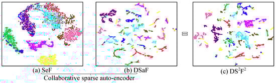
Figure 1. Visualization of features before and after collaborative fusion by t-SNE [33]: (a) raw spectral feature (SeF) (b) deep spatial feature (DSaF), and (c) deep spectral–spatial fusion feature (DS${}^2$F${}^2$). Take the University of Pavia dataset as example.

Manifold learning aims to keep the local neighborhood information of input space to the hidden space. Liao et al. [34] added graph regularized constraint in the auto-encoder model and proposed graph regularized auto-encoder (GAE) to maintain a certain spatial coherency of learning features. On the basis of GAE, we present a novel superpixel-based relational auto-encoder (S-RAE) for discriminant feature learning. As in the previous analysis, DSaF shows poor aggregation within the same class, but SeF present higher manifold. Therefore, intra-class consistency constraint, which is accomplished by graphical model structured in spectral domain, is added in S-RAE during the auto-encoder process of DSaF in the first layer before spectral–spatial fusion, so as to enhance its intra-class consistency. For the following defects of traditional graphical model: (1) pixel-level graph construction needs large matrix storage (which means the measurement matrix will be 21,025 × 21,025 for an image with size $145\times 145$); (2) sparse matrix that only consider neighborhood similarity is insensitive to boundary region; and (3) optimization of graph regularized constraint suffers high computational complexity. We utilize superpixel segmentation to reconstruct and optimize of graph regular term, which keeps the manifold in spectral domain, reduces the computational complexity, enhances boundary adaptability, and improves classification robustness.

The final feature extraction is completed by a collaborative auto-encoder of spectral and spatial features, and weighting fusion of multiscale features, so as to achieve feature presentation with high intra-class aggregation and inter-class difference. A large number of experimental results shows that S-RAE achieves desired effects in cohesive DSaF learning, meanwhile admirably assists spectral–spatial fusion and mutliscale feature extraction for more precise and finer target recognition.

The remainder of this paper is organized as follows. We introduce graph regular auto-encoder (GAE) in Section 2. Section 3 outlines our proposed S-RAE, containing model establishment and optimization solution. Section 4 introduces spectral–spatial fusion and the final mutliscale feature fusion (MS-RCAE). Section 5 gives experimental design, parameter analysis and method comparison in detail. Conclusion is involved in Section 6.

2. Graph Regularized Auto-Encoder (GAE)

Graph regularized auto-encoder (GAE) [34] assumes that if neighborhood pixels $x^{\left(i\right)}$ and $x^{\left(j\right)}$ are close to each other in low-dimensional manifold, their corresponding hidden representation $h^{\left(i\right)}$ and $h^{\left(j\right)}$ should also be close too. Thus, GAE adds a local invariant constraint to the cost function of auto-encoder (AE). Let the reconstruction cost of AE be:

$$J_{AE}\left(\theta \right)=\frac{1}{t}\sum _{i=1}^t\frac{1}{2}{∥x^{\left(i\right)}-{\widehat{x}}^{\left(i\right)}∥}^2+\frac{\lambda }{2}{∥W∥}^2,$$

(1)

where t is the total amount of input samples, $W=\left\{W_e,W_d\right\}$, and $\theta =\left\{W_e,b_e,W_d,b_d\right\}$ are all the training parameters in AE. ${∥W∥}_2$ is the weight penalty term and $\lambda$ is a balance parameter. The encoder and decoder is presented as

$$\begin{array}{c}\hfill h=\sigma \left(W_{e}x+b_e\right),\end{array}$$

(2)

$$\begin{array}{c}\hfill \widehat{x}=\sigma \left(W_{d}h+b_d\right).\end{array}$$

(3)

Thus, the cost function of GAE is

$$J_{GAE}\left(\theta \right)=J_{AE}\left(\theta \right)+\frac{\gamma }{2t}\sum _{i=1}^t\sum _{j=1}^t{v}_{ij}{∥h^{\left(i\right)}-h^{\left(j\right)}∥}^2,$$

(4)

where $\gamma$ is the weighting coefficient for graph regularization term, $v_{ij}$ records the distance between input variables $x^{\left(i\right)}$ and $x^{\left(j\right)}$. The closer the two variables in the input space, the larger the distance measurement $v_{ij}$, and thus forcing the greater similarity between $h^{\left(i\right)}$ and $h^{\left(j\right)}$ in the hidden representational layer.

Let $V={\left[v_{ij}\right]}_{t\times t}$ be a adjacency graph composed of the similarity measurement. Generally, V is constructed as a sparse matrix, which means only few neighbors (according to given scale) are connected in order to reduce storage. Here, the connectivity between samples can be given by kNN-graph or ϵ-graph method, etc., and weight between two connected samples be calculated by binary or heat kernel method, etc. [34].

Finally, the cost function can be expressed in the following matrix form:

$$J_{GAE}=\frac{1}{t}{∥X-\widehat{X}∥}_F^2+{∥W∥}_F^2+\frac{\gamma }{t}tr\left(HL{H}^T\right),$$

(5)

where $tr\left(·\right)$ is the trace of a matrix, L is the laplacian matrix, $L=D_1+D_2-2V$, $D_1$ and $D_2$ are $t\times t$ diagonal matrices with diagonal elements $d_{ii}^1={\sum }_{j=1}^t{v}_{ij}$ and $d_{jj}^2={\sum }_{i=1}^t{v}_{ij}$, respectively.

The parameter of $J_{GAE}$ can be solved by the stochastic gradient descent based iterative optimization algorithm.

$$\left\{{\theta }_e,{\theta }_d\right\}=argmin{J}_{GAE},$$

(6)

where ${\theta }_e=\left\{W_e,b_e\right\}$ and ${\theta }_d=\left\{W_d,b_d\right\}$ correspond to the parameters in encoding and decoding. Details please refer to [34].

3. Superpixel-Based Relational Auto-Encoder

DSaF, extracted by pre-trained filter banks in VGG-16, presents excellent inter-class separability, but also suffer terrible intra-class consistency. This phenomenon can hardly be compensated by the spectral–spatial fusion strategy. Amending DSaF with the manifold in spectral domain could effectively weaken this problem. GAE is a good method in capturing local manifolds, but the graph regular term in GAE contains a graph matrix V, which occupies plenty of storage, and increases the computational complexity in network training, even if batch processing under neighborhood pixels (as proposed in [34]). Additionally, a fixed-size neighborhood of randomly selected samples is prone to error in the boundary region. In order to avoid the calculation of graph matrix and interference of fixed neighborhood in GAE, we propose a superpixel-based relational auto-encoder (S-RAE) network. In this method, we firstly extract DSaFs by the transferred filter banks in VGG-16, and upsample them to have the same spatial dimension. Meanwhile, HSI, after spectral reduction and spatial downsampling, is segmented into superpixels in the spectral domain. We enhance the intra-class consistency of DSaFs by interrelationship constraints in each superpixel, which not only retain manifold well, but also consume little running time. A detailed process of our proposed S-RAE is summarized in Algorithm 1.

Algorithm 1: S-RAE.

Input: HSI data; Hidden size, sparsity $\rho$, regular parameter $\lambda$, $\beta$ for $J_{SAE}$; Superpixel clusters number and weight coefficient $\gamma$ for $J_R$; weighting parameter ${\alpha }_1$ and ${\alpha }_2$ for MS-RCAE.

1. The first three principal components from PCA of HSI are reserved as the inputs of VGG16;

2. Extract DSaF from the pre-trained filter banks in VGG16;

3. Upsample feature maps in the last pooling layer with 4 pixels stride by bilinear interpolation operation;

4. Normalize the raw spectral data and downsample with 8 pixels stride by average pooling;

5. Reserve the maximum principal component of the downsampled image after PCA, and do superpixel segmentation;

6. Separate the cross-region superpixels in the segmented image by connected graph method;

7. Learning cohesive DSaF by S-RAE (a) Take the feature from step 3 as the input, randomly initialized ${\theta }_e$ and ${\theta }_d$, and calculate the loss function (7); (b) Calculate the derivative of $J_{SAE}$ with respect to ${\theta }_e$ by Equations (16) and (18); (c) Calculate the derivative of $J_R$ with respect to ${\theta }_e$ by Equations (21) and (25); (d) Calculate the derivative of $J_{SRAE}$ with respect to ${\theta }_d$ by Equations (27) and (29); (e) Update all the parameters in $\theta$ by Equation (30);

8. Upsample the learned features of hidden layer to have a same scale with the input maps.

Output: Feature maps

3.1. Model Establishment

With the assumption that if two pixels, $x_e^{\left(i\right)}$ and $x_e^{\left(j\right)}$, are close in the raw spectral domain, their corresponding lower-dimensional representation of DSaF, $h_a^{\left(i\right)}$ and $h_a^{\left(j\right)}$, should present high similarity with great possibility as well. Thus, based on the loss function of sparse auto-encoder (SAE), we add one relational constraint in the hidden layer coding of DSaF to enhance its intra-class consistency, which is expressed as

$$\begin{array}{cc}\hfill J_{SRAE}\left({\theta }_e,{\theta }_d\right)& =J_{SAE}\left({\theta }_e,{\theta }_d\right)+J_R\left({\theta }_e\right)\hfill \end{array}$$

(7)

$$\begin{array}{cc}\hfill & =\frac{1}{t}\sum _{i=1}^t\frac{1}{2}{∥x_a^{\left(i\right)}-{\widehat{x}}_a^{\left(i\right)}∥}^2+\frac{\lambda }{2}{∥W∥}^2+\beta \sum _{j=1}^{n}KL\left(\rho ∥{\widehat{\rho }}_j\right)\hfill \end{array}$$

(8)

$$\begin{array}{cc}\hfill & +\gamma \frac{1}{\left|\mathsf{\Psi }\right|}\sum _{C_k\in \mathsf{\Psi }}\frac{1}{2\left(\left|C_k\right|\sim \right)}\sum _{1\le i\le j\le \left|C_k\right|}{∥h_a^{\left(i\right)}-h_a^{\left(j\right)}∥}^2,\hfill \end{array}$$

(9)

where Equation (8) is the loss function of SAE. KL (Kullback–Leibler) distance is introduced here for sparsity constraint,

$$KL\left(\rho ∥{\widehat{\rho }}_j\right)=\rho log\frac{\rho }{{\widehat{\rho }}_j}+\left(1-\rho \right)log\frac{1-\rho }{1-{\widehat{\rho }}_j},$$

(10)

in which ${\widehat{\rho }}_j=\frac{1}{t}{\displaystyle \sum _{i=1}^t}{h}_{a,j}^{\left(i\right)}$ is the average activation of all inputs in the j-th neuron. The proposed relational constraint is defined as in Equation (9). To establish neighborhood relationship adaptively, we utilize over-segmented superpixels, and do the relational constraint in each superpixel. In Equation (9), $C_k$ is a set of pixels in the k-th superpixel, $\mathsf{\Psi }$ is a set consisting of all the superpixels, and $\left|C_k\right|\sim$ means dectorial of the elements number of $C_k$.

Superpixel is usually defined as a region with consistent perception in the image, and is composed of the same target, which provides spatial support for region-based feature calculation [35]. In this paper, we build the spatial relationships by Liu et al.’s proposed clustering-based superpixel segmentation method [35], which includes two terms in its loss function: (1) Entropy rate of random walk on constructed graphs to obtain compact and homogeneous clusters, and (2) Balance term that encourages all the clusters with similar sizes. This method processes segmentation as a clustering problem, while our target is for consistency constraint of a neighborhood. Thus, a connected graph is utilized here and does a simple reprocessing for the segmented superpixels, which forces each superpixel block only containing pixels in contiguous region but not the cross-region. The superpixel segmentation is achieved on the maximum principal component of the original HSI after principal component analysis (PCA). With experimental verification, connected graph operation makes a parameter setting in superpixel segmentation extremely robust.

Figure 2 shows the difference between traditional AE, GAE, and our proposed S-RAE. Compared with GAE, S-RAE does not build neighborhood relationships with the input data. As analyzed in Section 1, DSaF extracted by transferred deep filter banks presents strong inter-class separability, but poor intra-class aggregation, while the spectral feature can just compensate for this deficiency. Thus, in this paper, we build neighborhood relations in the spectral domain (represented by blue dots in Figure 2), and do the neighborhood consistency constraint for spatial feature. Besides, the metric matrix V in the loss function (4) of GAE is canceled from the relational constraint term in Equation (9), and relationships in S-RAE only involve pixels in each superpixels, instead of crossing between them. The purpose of relational auto-encoder in this paper is to learn spatial features with highly intra-class consistency, thus we only need to guarantee a minimum difference of the hidden layer features within each superpixel, but without any additional measurement of their similarity. Meanwhile, DSaF has stronger inter-class difference, so there is no need for further constraint or optimization.

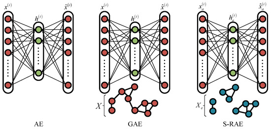
Figure 2. Comparison of AE, GAE, and our proposed S-RAE.

3.2. Model Optimization

The parameters optimization of ${\theta }_e$ and ${\theta }_d$ in Equation (7) could be achieved by gradient descent algorithm. For the parameter ${\theta }_e$ in the encoder part, we have

$$\frac{\partial J_{SRAE}\left({\theta }_e,{\theta }_d\right)}{\partial {\theta }_e}=\frac{\partial J_{SAE}\left({\theta }_e,{\theta }_d\right)}{\partial {\theta }_e}+\gamma \frac{\partial J_R\left({\theta }_e\right)}{\partial {\theta }_e},$$

(11)

where ${\theta }_e$ is in the reconstitution of ${\widehat{x}}_a^{\left(i\right)}$,

$${\widehat{x}}_a^{\left(i\right)}=\sigma \left(W_d\sigma \left(W_e{x}_a^{\left(i\right)}+b_e\right)+b_d\right),$$

(12)

the weight penalty term ${∥W∥}_2$, and the constraint of hidden layer $h_a^{\left(i\right)}$,

$$h_a^{\left(i\right)}=\sigma \left(W_e{x}^{\left(i\right)}+b_e\right).$$

(13)

We use sigmoid $\sigma \left(x\right)=1/\left(1+e^{-x}\right)$ as their activation function in all the encoder and decoder part, and its derivation can be expressed as

$${\sigma }^{\prime }\left(x\right)=\sigma \left(x\right)\left[1-\sigma \left(x\right)\right].$$

(14)

Thus, in the part of SAE, we have

$$\begin{array}{cc}\hfill \frac{\partial J_{SAE}\left({\theta }_e,{\theta }_d\right)}{\partial W_e}& =\frac{\partial J_{AE}\left({\theta }_e,{\theta }_d\right)}{\partial W_e}+\beta \frac{\partial }{\partial W_e}\sum _{j=1}^{n}KL\left(\rho ∥{\widehat{\rho }}_j\right)\hfill \\ \hfill & =-\frac{1}{t}\sum _{i=1}^t\left\{W_d^T\times \left[\left(x^{\left(i\right)}-{\widehat{x}}^{\left(i\right)}\right)\odot f\left({\widehat{x}}^{\left(i\right)}\right)\right]\odot f\left(h^{\left(i\right)}\right)\right\}\times {\left(x^{\left(i\right)}\right)}^T\hfill \end{array}$$

(15)

$$\begin{array}{cc}\hfill & +\lambda W_e+\frac{\beta }{t}\sum _{i=1}^t\left\{\left(-\frac{\rho }{\widehat{\rho }}+\frac{1-\rho }{1-\widehat{\rho }}\right)\odot f\left(h^{\left(i\right)}\right)\right\}\times {\left(x^{\left(i\right)}\right)}^T,\hfill \end{array}$$

(16)

where $\widehat{\rho }\in {\mathcal{R}}^n$ is the sparsity of n neurons in hidden layer, $f\left(x\right)=x\odot \left(1-x\right)$, and ⊙ represents dot product operation of matrix. The derivative of $J_{SAE}$ with respect to $b_e$ can be obtained as

$$\begin{array}{cc}\hfill \frac{\partial J_{SAE}\left({\theta }_e,{\theta }_d\right)}{\partial b_e}& =\frac{\partial J_{AE}\left({\theta }_e,{\theta }_d\right)}{\partial b_e}+\beta \frac{\partial }{\partial b_e}\sum _{j=1}^{n}KL\left(\rho ∥{\widehat{\rho }}_j\right)\hfill \\ \hfill & =-\frac{1}{t}\sum _{i=1}^t{W}_d^T\times \left[\left(x^{\left(i\right)}-{\widehat{x}}^{\left(i\right)}\right)\odot f\left({\widehat{x}}^{\left(i\right)}\right)\right]\odot f\left(h^{\left(i\right)}\right)\hfill \end{array}$$

(17)

$$\begin{array}{cc}\hfill & +\frac{\beta }{t}\sum _{i=1}^t\left(-\frac{\rho }{\widehat{\rho }}+\frac{1-\rho }{1-\widehat{\rho }}\right)\odot f\left(h^{\left(i\right)}\right).\hfill \end{array}$$

(18)

For the relational constraint part, we rewrite the loss function (9) as

$$\begin{array}{cc}\hfill J_R& =\frac{1}{\left|\mathsf{\Psi }\right|}\sum _{C_k\in \mathsf{\Psi }}\frac{1}{2\left(\left|C_k\right|\sim \right)}\sum _{1\le i\le j\le \left|C_k\right|}{∥h_a^{\left(i\right)}-h_a^{\left(j\right)}∥}^2\hfill \\ \hfill & =\sum {∥\sigma \left(W_e{x}^{\left(i\right)}+b_e\right)-\sigma \left(W_e{x}^{\left(j\right)}+b_e\right)∥}^2.\hfill \end{array}$$

(19)

Thus the partial derivation of $W_e$ could be

$$\frac{\partial J_R}{\partial W_e}=\sum \left(h_a^{\left(i\right)}-h_a^{\left(j\right)}\right)\odot \left[f\left(h^{\left(i\right)}\right)\times {\left(x^{\left(i\right)}\right)}^T-f\left(h^{\left(j\right)}\right)\times {\left(x^{\left(j\right)}\right)}^T\right].$$

(20)

Even if the neighborhood relationship is established within the superpixel, measuring distance per pixel is still computationally expensive. Therefore, we relax the pixel-wise similarity constraint to a minimum of mean deviation (M.D.) in each superpixel block. Thus, the derivative of Equation (20) can be approximated as

$$\begin{array}{cc}\hfill \frac{\partial J_R}{\partial W_e}& \approx \frac{1}{\left|\mathsf{\Psi }\right|}\sum _{C_k\in \mathsf{\Psi }}\frac{1}{\left|C_k\right|}\sum _{i\in C_k}\left(h^{\left(i\right)}-{\overline{h}}_a^{\left(C_k\right)}\right)\odot f\left(h^{\left(i\right)}\right)\times {\left(x^{\left(i\right)}\right)}^T-f\left({\overline{h}}_a^{\left(C_k\right)}\right)\times {\left({\overline{x}}^{\left(C_k\right)}\right)}^T,\hfill \end{array}$$

(21)

where

$$\begin{array}{cc}\hfill {\overline{h}}_a^{\left(C_k\right)}& =\frac{1}{\left|C_k\right|}\sum _{i\in C_k}{h}_a^{\left(i\right)},\hfill \end{array}$$

(22)

$$\begin{array}{cc}\hfill {\overline{x}}_a^{\left(C_k\right)}& =\frac{1}{\left|C_k\right|}\sum _{i\in C_k}{x}_a^{\left(i\right)}.\hfill \end{array}$$

(23)

Likewise, we can obtain the derivative of $J_R$ with respect to $b_e$ as

$$\begin{array}{cc}\hfill \frac{\partial J_R}{\partial b_e}& =\sum \left(h_a^{\left(i\right)}-h_a^{\left(j\right)}\right)\odot \left[f\left(h_a^{\left(i\right)}\right)-f\left(h_a^{\left(j\right)}\right)\right]\hfill \end{array}$$

(24)

$$\begin{array}{cc}\hfill & \approx \frac{1}{\left|\mathsf{\Psi }\right|}\sum _{C_k\in \mathsf{\Psi }}\frac{1}{\left|C_k\right|}\sum _{i\in C_k}\left(h_a^{\left(i\right)}-{\overline{h}}_a^{\left(C_k\right)}\right)\odot \left[f\left(h_a^{\left(i\right)}\right)-f\left({\overline{h}}_a^{\left(C_k\right)}\right)\right].\hfill \end{array}$$

(25)

The relational regularization and sparse constraint in Equation (7) are mainly directed at neurons in the hidden layer. Thus, the optimization of parameter set ${\theta }_d$ is only relevant to $J_{AE}$, so we have

$$\begin{array}{cc}\hfill \frac{\partial J_{SRAE}\left({\theta }_e,{\theta }_d\right)}{\partial W_d}& =\frac{\partial J_{AE}\left({\theta }_e,{\theta }_d\right)}{\partial W_d}\hfill \end{array}$$

(26)

$$\begin{array}{cc}\hfill & =\frac{1}{t}\sum _{i=1}^t\left(x^{\left(i\right)}-{\widehat{x}}^{\left(i\right)}\right)\times \frac{\partial {\left(x^{\left(i\right)}-{\widehat{x}}^{\left(i\right)}\right)}^T}{\partial W_d}+\lambda W_d,\hfill \end{array}$$

(27)

and

$$\begin{array}{cc}\hfill \frac{\partial J_{SRAE}\left({\theta }_e,{\theta }_d\right)}{\partial b_d}& =\frac{\partial J_{AE}\left({\theta }_e,{\theta }_d\right)}{\partial b_d}\hfill \end{array}$$

(28)

$$\begin{array}{cc}\hfill & =-\frac{1}{t}\sum _{i=1}^t\left(x^{\left(i\right)}-{\widehat{x}}^{\left(i\right)}\right)\odot f\left({\widehat{x}}^{\left(i\right)}\right).\hfill \end{array}$$

(29)

Finally, all parameters $\theta =\left\{W_e,b_e,W_d,b_d\right\}$ are updated and optimized by the following iterative formula,

$${\theta }^{\left(k+1\right)}={\theta }^{\left(k\right)}-\tau {\left.\frac{\partial J_{SRAE}\left({\theta }_e,{\theta }_d\right)}{\partial \theta }\right|}_{\theta ={\theta }^{\left(k\right)}}.$$

(30)

4. Multiscale Spectral-Spatial Feature Fusion

Neighborhood constraint in S-RAE makes DSaF with strong intra-class consistency. However, transferring pre-trained (by natural images) deep network parameters still hard to keep the raw spectral features of hyperspectral images. Therefore, as we do in [32], one layer of collaborative sparse AE is added to the hidden layer of the proposed S-RAE network for fusing the spectral–spatial feature, which is abbreviated as S-RCAE and given by

$$\begin{array}{cc}\hfill J_{S-RCAE}\left({\theta }_e,{\theta }_d\right)& =\frac{1}{t}\sum _{i=1}^t\frac{1}{2}\left(∥x_e^{\left(i\right)}-{\widehat{x}}_e^{\left(i\right)}∥+∥h_{\tilde{a}}^{\left(i\right)}-{\widehat{h}}_{\tilde{a}}^{\left(i\right)}∥\right)\hfill \\ \hfill & +\frac{\lambda }{2}\left({∥W_e∥}_2+{∥W_d∥}_2\right)+\beta \sum _{j=1}^{n}KL\left(\rho ∥{\widehat{\rho }}_j\right),\hfill \end{array}$$

(31)

where $h_{\tilde{a}}^{\left(i\right)}$ is the normalization of hidden layer $h_a^{\left(i\right)}$ in S-RAE, and $x_e^{\left(i\right)}$ is the spectral features.

Besides, we still use the last three convolution modules in VGG-16 network to extract multiscale DSaFs and do spectral–spatial fusion by S-RCAE in each scale. Finally, we get the highly discriminant spectral–spatial features through the multiscale weighting fusion. Let $X_{P5}$, $X_{P4}$, $X_{P3}$ be spectral–spatial features obtained from the three scales, pool5, pool4, and pool3, respectively. Thus, the weighting fusion of them can be represented as

$$X={\alpha }_2{X}_{P3}+\left(1-{\alpha }_2\right)\left({\alpha }_1{X}_{P4}+\left(1-{\alpha }_1\right)X_{P5}\right),$$

(32)

where ${\alpha }_1$ and ${\alpha }_2$ are weighting parameters. X is the final discriminant feature obtained by our proposed MS-RCAE. Figure 3 gives the algorithm flow.

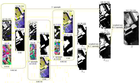
Figure 3. Illustration of the proposed MS-RCAE (All the sizes are subject to the digital markers). A case of the Salinas dataset.

5. Experiments

5.1. Data Sets and Quantitative Metrics

In this section, we introduce four public databases to experimentally confirm the advantages of our proposed MS-RCAE for HSIC. They respectively are:

Indian Pines: This data consists image of size $145\times 145$ with spatial resolution of 20 m per pixel and 200 spectral bands (20 water absorption bands be removed) in the wavelength range from $0.4$ to 2.5 $\mathsf{\mu }$m. The ground truth available contains 16 classes.

University of Pavia: This data includes image of size $610\times 340\times 103$ with geometric resolution of 1.3 m and spectral coverage ranging from $0.43$ to 0.86 $\mathsf{\mu }$m. The ground truth available differentiates 9 classes.

Salinas: This data consists of image of size $512\times 217$ with high spatial resolution of 3.7 m per pixel, and the spectral reflectance bands is 204 after 20 water absorption bands moved. 16 classes is available in the ground truth.

Kennedy Space Center (KSC): This data consists image of size $512\times 614$ with spatial resolution of 18 m per pixel and 176 spectral bands (removed water absorption and low SNR bands) in 10 nm width with center wavelengths from $0.4$ to 2.5 $\mathsf{\mu }$m. 13 classes is available in the ground truth.

Figure 4 shows the pseudocolor image and corresponding ground truth of those datasets, respectively. To evaluate the proposed MS-RCAE method qualitatively, we select support vector machine (SVM) [36] as classifier for all the feature learning-based method, and use linear kernel function with penalty factor uniformly equal to 10. Overall accuracy (OA), average accuracy (AA), and Kappa coefficient are adopted to statistical evaluation of the results. All experiments in this paper are repeated 20 times with randomly selected train samples from the labeled pixels in each dataset, and we report the average accuracy across the 20 folds.

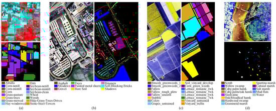
Figure 4. Pseudo-color and ground references for the following datasets. (a) Indian Pines; (b) University of Pavia; (c) Salinas; (d) KSC.

5.2. Parameters Analysis

In our proposed S-RAE and MS-RCAE methods, the parameters to be set empirically mainly include: the number of superpixel clusters and the weight coefficient $\gamma$ for relational regular term in Equation (9), and the weighting parameters in Equation (32) for multiscale fusion. To analyze the influence of parameter setting on classification accuracy, we randomly select 5% labeled samples from Indian Pines dataset for model training, and the rest 95% as test samples. For other three datasets, we randomly select 10 labeled pixels from each class as training samples, and all the others for testing.

We chose the number of superpixel clusters in the range from 10 to 80, weight coefficient $\gamma$ from 0 to 30, and analyze the two parameters simultaneously here. Since the size of Indian Pines data is too small after $4\times$ downsampling, and the over-segmentation is extremely unbalanced when the number of clusters over 30. Therefore, this group of parameter analysis is primarily conducted on the other three datasets. To further illustrate the parameter robustness, we do the dimension reduction of DSaF by S-RAE under different parameters at the pool5 and pool3 layer of VGG-16, respectively. Then, the processed features are upsampled by corresponding scales, and classified by SVM. The experimental results are shown in Figure 5, and features extracted at different layers are annotated as S-RAE-P5 and S-RAE-P3, respectively. As seen from the results, S-RAE achieves relatively stable classification accuracy when the value of $\gamma$ is greater than 15, and there is no significant influence when the number of clusters is set between 10 and 80. Therefore, we set the number of clusters at 60 and the regular parameter $\gamma =15$ in all experiments, except for Indian Pines data with 30 clusters.

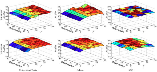
Figure 5. Effect of initial superpixel clusters number and weight coefficient $\gamma$ on classification accuracy.

We further examine how the proposed MS-RCAE behaves when the weighting parameters ${\alpha }_1$ and ${\alpha }_2$ in Equation (32) change from 0.2 to 0.7. As the results shown in Figure 6, images with finer spatial texture will be more beneficial to the shallow local feature descriptor, while those with smooth distribution but complex semantic information can be more inclined to the deep global descriptor, such as the University of Pavia data benefits from a larger weight on features from pool4, Salinas and KSC data prefer to pool5, while Indian Pine depends equally on the three scale layers. Thus, we set ${\alpha }_1={\alpha }_2=0.5$ for Indian Pine, ${\alpha }_1=0.2$, ${\alpha }_2=0.6$ for University of Pavia, ${\alpha }_1={\alpha }_2=0.4$ for Salinas and KSC, respectively.

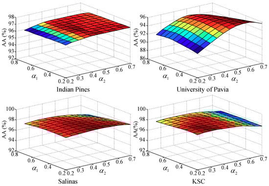
Figure 6. Effect of weighting parameters ${\alpha }_1$ and ${\alpha }_2$ on classification accuracy.

5.3. Stepwise Evaluation of the Proposed Strategies

The main innovation in this paper is S-RAE for more discriminative feature learning. In order to verify its effectiveness, we severally compare the classification accuracy of DSaF processed by S-RAE and SAE, as well as deep spectral–spatial fusion feature by S-RCAE and CAE in [32], respectively. All experiments here are conducted on three experimental datasets except Indian Pines. To enhance the persuasiveness, we present the results of an increasing number of training samples from 3 to 50.

To analyze the effectiveness of our proposed S-RAE, SAE and S-RAE are compared to reduce the dimension of deep spatial features extracted from the last three convolutional modules in VGG-16, all of which are abbreviated as SAE-P5, SAE-P4, SAE-P3, and S-RAE-P5, S-RAE-P4, S-RAE-P3, respectively. Classification results, as shown in Figure 7, show that S-RAE gets great improvement on each scale features and all the datasets compared with the traditional SAE. This experiment strongly indicates that using the potential manifold in the spectral domain as a consistency constraint effectively improves the intra-class aggregation of the deep spatial feature, and thus the high discriminability of each target

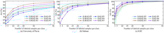
Figure 7. Comparison of classification results from deep spatial feature preprocessed by SAE and S-RAE on datasets of (a) University of Pavia, (b) Salinas, and (c) KSC.

In addition, we further demonstrate the superiority of S-RAE from comparison of the spectral–spatial fusion features extracted by S-RCAE and CAE in [32]. Here, we also do the experiment on three scale layers, which are named as S-RCAE-P5, S-RCAE-P4, S-RCAE-P3, and correspondingly compared with CAE-P5, CAE-P4, CAE-P3, as well as the final method MS-RCAE. From the experimental results as in Figure 8, we can conclude that modification of DSaF by S-RAE could assist the collaborative network more effectively learning commonalities between spatial and spectral features in each scale, and excellently enhancing discriminability and robustness of learned features, such as more precise classification accuracy with a few training samples. Meanwhile, weighting fusion of multiscale features further improves their classification accuracy, particularly outstanding on University of Pavia dataset.

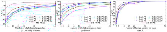
Figure 8. Comparison of classification results from spectral–spatial feature learned by CAE, S-RCAE, and multiscale feature by MS-RCAE on datasets of (a) University of Pavia, (b) Salinas, and (c) KSC.

5.4. Comparison with Other Feature Extraction Algorithm

In this section, we compare our proposed method MS-RCAE with existing unsupervised feature extraction and deep learning-based methods through quantitative analysis and visual comparison, including recursive filtering (RF) [37] and intrinsic image decomposition (IID) [38] based unsupervised feature extraction method, joint-sparse auto-encoder (J-SAE) [5], guided filter-fast sparse auto-encoder (GF-FSAE) [8], 3-D CNN based method (3D-CNN) [4], deep spatial distribution prediction (MS${}^3$FE) algorithm [20], and deep multiscale spectral–spatial feature fusion (DMS${}^3$F${}^2$) [32]. The parameters of all comparison methods in this section are set according to the corresponding references.

Table 1, Table 2, Table 3 and Table 4 respectively counts the classification accuracy of all comparison methods on the four experimental datasets, while Figure 9, Figure 10, Figure 11 and Figure 12 shows the corresponding classification maps of all the pixels. Numerical experiments demonstrate that our proposed method, compared with other methods, achieves the highest accuracy on Indian Pines, University of Pavia, and KSC datasets, though it does not achieve the best results on every category, the accuracy almost above 95%. Although the results on Salinas data are still relatively worse than IID, it is comparable to the best results, and has more promotion compared with DMS${}^3$F${}^2$. This well illustrates the effectiveness of our proposed superpixel-based neighborhood consistency constraint. As can be seen from the classification maps, besides reasonable semantic recognition, our method completes finer and more accurate edge segmentation, such as finer marsh recognition across the sea in KSC, more regular boundaries in Salinas data that with more adjacent boundary marking.

Table 1. Classification accuracies of the Indian Pines dataset obtained by each comparison methods. The best results are highlighted in bold font.

Class	# Samples		Classification Methods
	Train	Test	SVM	IID	RF	J-SAE	GF-FSAE	3D-CNN	MS${}^3$FE	DMS${}^3$F${}^2$	MS-RCAE
1	3	43	34.65	97.98	94.53	97.56	61.74	60.98	95.47	97.44	96.51
2	72	1356	65.38	83.38	92.90	85.68	67.19	78.60	88.84	96.23	96.39
3	42	788	43.87	89.75	93.05	90.50	74.00	87.42	93.78	96.55	96.51
4	12	225	34.64	86.50	90.07	68.22	58.69	88.32	92.87	96.00	96.49
5	25	458	81.08	94.11	92.72	78.98	89.20	80.60	92.31	93.49	94.65
6	38	692	93.16	97.64	99.34	95.11	98.37	92.98	98.89	99.62	99.65
7	2	26	65.19	96.28	98.46	60.00	51.54	68.00	96.54	99.62	99.62
8	25	453	95.20	100	99.67	100	99.28	95.57	99.22	100	100
9	2	18	34.17	99.63	88.89	44.44	47.22	77.78	100	95.00	96.67
10	49	923	61.16	84.07	92.38	83.43	75.14	76.91	92.32	94.54	94.43
11	124	2331	78.29	86.72	96.33	95.24	60.53	85.42	98.72	98.82	98.79
12	31	562	44.77	81.49	91.93	91.17	65.23	82.52	92.78	94.11	94.56
13	11	194	97.40	98.97	99.10	91.30	94.48	96.20	98.69	96.39	98.56
14	65	1200	95.74	99.20	98.28	97.01	99.31	99.30	99.95	99.06	99.28
15	19	367	42.33	89.52	93.96	95.98	90.89	89.94	99.46	98.69	98.96
16	5	88	85.34	90.04	98.30	86.75	81.42	85.54	93.81	92.84	98.41
AA (%)			65.77	92.21	94.99	85.09	75.89	84.13	95.85	96.78	97.47
OA (%)			72.04	89.70	95.22	90.89	76.77	86.43	95.71	97.30	97.53
Kappa			0.6775	0.8828	0.9455	0.8960	0.7442	0.8450	0.9510	0.9693	0.9718

Table 2. Classification accuracies of University of Pavia dataset obtained by each comparison methods. The best results are highlighted in bold font.

Class	# Samples		Classification Methods
	Train	Test	SVM	IID	RF	J-SAE	GF-FSAE	3D-CNN	MS${}^3$FE	DMS${}^3$F${}^2$	MS-RCAE
1	10	6621	62.75	80.40	65.55	58.25	75.60	57.48	87.67	92.80	95.15
2	10	18,639	58.75	88.02	84.34	86.19	76.36	87.80	87.38	91.06	94.17
3	10	2089	46.45	94.25	82.93	58.34	83.83	53.20	97.87	97.95	98.95
4	10	3054	91.41	92.49	77.41	95.78	95.34	89.19	88.06	91.90	94.30
5	10	1335	99.77	99.98	99.19	100	94.84	95.09	99.98	99.62	99.81
6	10	5019	59.20	98.28	93.47	69.99	88.01	75.70	95.36	97.27	98.44
7	10	1320	88.18	99.01	88.24	95.15	85.77	89.08	99.50	98.48	99.37
8	10	3672	73.23	86.14	67.62	57.75	81.68	86.95	93.47	95.59	95.70
9	10	937	99.57	84.23	66.90	96.95	93.78	92.88	98.69	97.39	97.75
AA (%)			75.48	91.42	80.63	79.82	86.14	80.82	94.22	95.78	97.07
OA (%)			65.59	89.14	80.70	75.66	81.05	80.39	90.51	93.52	95.63
Kappa			0.5765	0.8599	0.7513	0.6823	0.7603	0.7454	0.8781	0.9165	0.9435

Table 3. Classification accuracies of the Salinas dataset obtained by each comparison methods. The best results are highlighted in bold font.

Class	# Samples		Classification Methods
	Train	Test	SVM	IID	RF	J-SAE	GF-FSAE	3D-CNN	MS${}^3$FE	DMS${}^3$F${}^2$	MS-RCAE
1	10	1999	96.81	100	100	100	97.51	78.68	97.97	97.09	99.99
2	10	3716	91.91	99.95	97.87	100	99.04	75.50	97.40	100	100
3	10	1966	88.71	100	99.99	94.79	100	97.09	99.63	97.58	98.55
4	10	1384	99.28	99.29	98.94	98.84	99.41	99.85	99.45	98.79	99.65
5	10	2668	95.97	98.88	95.93	96.61	97.90	97.07	97.61	94.39	95.34
6	10	3949	99.74	99.86	99.60	100	99.84	99.85	99.81	99.79	99.95
7	10	3569	99.51	99.86	99.02	95.98	99.80	99.72	99.94	99.10	99.85
8	10	11,261	61.09	94.97	87.62	68.59	84.62	29.83	92.50	85.66	93.30
9	10	6193	97.85	98.89	99.99	98.53	99.81	95.05	98.31	99.63	99.69
10	10	3268	76.73	96.84	98.40	88.80	89.10	92.33	92.21	95.64	96.96
11	10	1058	91.55	99.73	96.61	99.14	95.20	100	97.37	99.15	99.89
12	10	1917	97.52	100	97.13	99.11	99.13	99.42	99.18	97.22	99.42
13	10	906	95.27	98.37	97.13	98.21	92.23	96.99	96.69	98.17	99.77
14	10	1060	91.30	96.88	96.75	99.05	94.08	100	94.52	98.36	99.28
15	10	7258	58.03	93.29	97.00	53.08	91.27	86.81	96.15	90.13	92.12
16	10	1797	91.92	99.75	95.77	98.27	97.02	94.18	99.53	99.64	99.99
AA (%)			89.57	98.53	97.36	93.04	95.98	90.15	97.39	96.90	98.36
OA (%)			82.45	97.53	96.02	85.43	94.15	79.49	96.57	94.61	96.98
Kappa			0.8052	0.9725	0.9558	0.8379	0.9350	0.7746	0.9619	0.9401	0.9663

Table 4. Classification accuracies of the KSC dataset obtained by each comparison methods. The best results are highlighted in bold font.

Class	# Samples		Classification Methods
	Train	Test	SVM	IID	RF	J-SAE	GF-FSAE	3D-CNN	MS${}^3$FE	DMS${}^3$F${}^2$	MS-RCAE
1	10	751	81.91	73.88	83.93	93.66	86.60	91.50	94.10	96.36	99.19
2	10	233	74.59	74.06	67.30	73.99	83.67	100	93.24	98.37	99.10
3	10	246	82.99	95.77	99.51	84.75	72.09	85.59	98.70	98.50	99.88
4	10	242	40.21	74.71	77.87	39.66	60.56	60.34	97.62	94.55	95.87
5	10	151	40.36	82.65	97.15	58.16	52.45	100	86.49	98.08	98.08
6	10	219	51.16	99.82	86.67	77.03	30.82	94.26	99.82	100	100
7	10	95	78.53	100	99.32	100	69.63	100	100	100	100
8	10	421	73.97	95.49	95.12	77.62	89.26	85.89	93.57	94.21	98.26
9	10	510	81.14	83.76	89.73	90.60	86.62	73.80	94.63	98.02	98.35
10	10	394	79.12	95.30	94.43	88.02	95.75	99.48	88.85	100	100
11	10	409	91.49	99.58	99.27	97.99	98.22	93.23	96.32	100	100
12	10	493	86.90	95.43	91.45	92.55	83.09	83.23	96.98	97.63	100
13	10	917	99.91	99.99	100	100	99.44	100	100	100	100
AA (%)			74.02	90.03	90.90	82.62	77.55	89.79	95.41	98.13	99.12
OA (%)			80.58	90.17	91.62	87.54	84.63	89.90	95.71	98.10	99.26
Kappa			0.7840	0.8909	0.9067	0.8609	0.8283	0.8876	0.9523	0.9788	0.9918

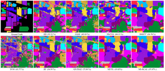
Figure 9. Classification maps of the Indian Pine dataset obtained by different methods (AA).

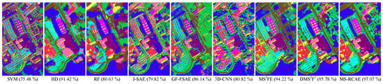
Figure 10. Classification maps of the University of Pavia dataset obtained by different methods (AA).

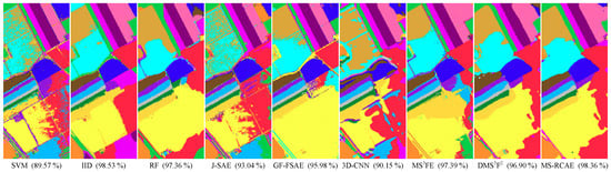
Figure 11. Classification maps of the Salinas dataset obtained by different methods (AA).

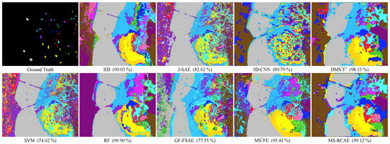
Figure 12. Classification maps of the KSC dataset obtained by different methods (AA).

Our method is mainly based on auto-encoder network, so we further compare the execution time of our proposed MS-RCAE with the SAE-based method, J-SAE [5], GF-FSAE [8], and DMS${}^3$F${}^2$ [32], as well as two CNN-based method, 3D-CNN [4] and MS${}^3$FE [20]. As Table 5 shows, 3D-CNN needs training lots of convolutional parameters, so it consume the most time and is recorded on the order of minutes. MS${}^3$FE extract deep features by the pre-trained FCN that with no training, so spend the least amount of time. To learn more discriminant feature, J-SAE and GF-FSAE all construct four hidden layers, while DMS${}^3$F${}^2$ and our method MS-RCAE only need two hidden layers with less neurons and iteration (though contain three submodules for multiscale fusion), they take almost twice as long time than the latter. From the results, we can conclude that superpixel-based relational constraint only adds a slight computational burden to MS-RCAE compared with DMS${}^3$F${}^2$, but significant improvement in classification accuracy.

Table 5. Execution Time of Different Methods on the Four Data Sets.

Datasets\Methods	MS-RCAE (s)	J-SAE (s)	GF-FSAE (s)	DMS${}^3$F${}^2$ (s)	3D-CNN (m)	MS${}^3$FE (s)
Indian Pines	163.45	310.94	247.69	132.12	41.24	0.56
University of Pavia	146.99	274.30	298.48	127.76	23.71	2.30
Salinas	194.69	305.23	282.85	160.43	50.53	1.79
KSC	291.70	430.78	291.89	225.71	44.51	3.72

To verify the stability advantages of our method, we further exhibit how classification accuracy changes with the increasing number of training samples on the University of Pavia, Salinas, and KSC datasets (see Figure 13, Figure 14 and Figure 15). Here, we randomly select training samples from each class, and let the number gradually increase from 3 to 50. The experimental results show that our proposed MS-RCAE method is superior to other comparison methods, especially in the case of small samples. Accuracy on Salinas data is still slightly worse than method IID. However, compared to other auto-encoder-based methods, such as J-SAE, GF-FSAE, and DMS${}^3$F${}^2$, our method shows significant advantages, particularly gets a big boost under less sample training conditions, which further illustrate that superpixel-based relational auto-encoder has a certain contribution to the discriminant feature extraction. In addition, although IID method achieves the highest classification accuracy on Salinas, it is not outstanding on the other datasets, and lower than our method by at least 5 percent, while our proposed MS-RCAE is only about 0.2 percent below IID on Salinas. This further indicates that our proposed method has certain universality.

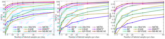
Figure 13. Effect of the number of training samples on classification accuracy for the University of Pavia dataset.

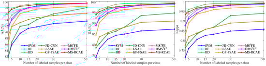
Figure 14. Effect of the number of training samples on classification accuracy for the Salinas dataset.

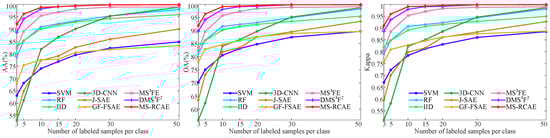
Figure 15. Effect of the number of training samples on classification accuracy for the KSC dataset.

6. Conclusions

In this paper, we propose a superpixel-based relational auto-encoder method to learn deep spatial features with high intra-class consistency. Firstly, we transferred the pre-trained filter banks in VGG-16 to extract deep spatial information of HSI. Then, the proposed S-RAE is utilized to reduce the dimensionality of the extracted deep feature. Based on the spectral feature with high intra-class consistency and deep spatial features with strong inter-class separability, we utilize the manifold relations in the spectral domain, and build a superpixel-based consistency constraint on the deep spatial feature to enhance its intra-class consistency. In addition, the obtained deep feature is further fused with the raw spectral feature by a collaborative auto-encoder, and the multiscale spectral–spatial features learned from the last three convolution modules in VGG-16 are weighting fused to achieve the final feature representation (MS-RCAE). To evaluate the proposed method in this paper qualitatively, we utilize SVM as a unified classifier to classify the extracted features. Extensive experiments on four public datasets demonstrate the superior performance of our proposed method, especially under the condition of small samples.

There is still plenty of room for improvement, such as more reasonable multiscale feature fusion strategies to maximize the advantages of each scale, more concise steps in representative feature learning, and a parallel computing strategy to speed up the calculation efficiency and enhance the demands of real-time performance.

References

- Zhang, L.; Zhang, L.; Du, B. Deep learning for remote sensing data: A technical tutorial on the state of the art. IEEE Geosci. Remote Sens. Mag. 2016, 4, 22–40. [Google Scholar] [CrossRef]
- Jiao, L.; Zhao, J.; Yang, S.; Liu, F. Deep learning, Optimization and Recognition; Tsinghua University Press: Beijing, China, 2017. [Google Scholar]
- Hu, W.; Huang, Y.; Wei, L.; Zhang, F.; Li, H. Deep convolutional neural networks for hyperspectral image classification. J. Sens. 2015, 2015, 1–12. [Google Scholar] [CrossRef]
- Chen, Y.; Jiang, H.; Li, C.; Jia, X.; Ghamisi, P. Deep feature extraction and classification of hyperspectral images based on convolutional neural networks. IEEE Trans. Geosci. Remote Sens. 2016, 54, 6232–6251. [Google Scholar] [CrossRef]
- Chen, Y.; Lin, Z.; Zhao, X.; Wang, G.; Gu, Y. Deep learning-based classification of hyperspectral data. IEEE J. Sel. Top. Appl. Earth Observ. Remote Sens. 2014, 7, 2094–2107. [Google Scholar] [CrossRef]
- Xing, C.; Ma, L.; Yang, X. Stacked denoise autoencoder based feature extraction and classification for hyperspectral images. J. Sens. 2016, 2016, 1–10. [Google Scholar] [CrossRef]
- Zabalza, J.; Ren, J.; Zheng, J.; Zhao, H.; Qing, C.; Yang, Z.; Du, P.; Marshall, S. Novel segmented stacked autoencoder for effective dimensionality reduction and feature extraction in hyperspectral imaging. Neurocomputing 2016, 185, 1–10. [Google Scholar] [CrossRef]
- Wang, L.; Zhang, J.; Liu, P.; Choo, K.K.R.; Huang, F. Spectral–spatial multi-feature-based deep learning for hyperspectral remote sensing image classification. Soft Comput. 2017, 21, 213–221. [Google Scholar] [CrossRef]
- Jiao, L.; Liu, F. Wishart deep stacking network for fast POLSAR image classification. IEEE Trans. Image Process. 2016, 25, 3273–3286. [Google Scholar] [CrossRef]
- Guo, Y.; Jiao, L.; Wang, S.; Wang, S.; Liu, F. Fuzzy Sparse Autoencoder Framework for Single Image Per Person Face Recognition. IEEE Trans. Cybern. 2018, 48, 2402–2415. [Google Scholar] [CrossRef]
- Chen, Y.; Zhao, X.; Jia, X. Spectral–spatial classification of hyperspectral data based on deep belief network. IEEE J. Sel. Top. Appl. Earth Observ. Remote Sens. 2015, 8, 2381–2392. [Google Scholar] [CrossRef]
- Zhong, P.; Gong, Z.; Li, S.; Schönlieb, C.B. Learning to diversify deep belief networks for hyperspectral image classification. IEEE Trans. Geosci. Remote Sens. 2017, 55, 3516–3530. [Google Scholar] [CrossRef]
- Liu, F.; Jiao, L.; Hou, B.; Yang, S. POL-SAR Image Classification Based on Wishart DBN and Local Spatial Information. IEEE Trans. Geosci. Remote Sens. 2016, 54, 3292–3308. [Google Scholar] [CrossRef]
- Zhao, Z.; Jiao, L.; Zhao, J.; Gu, J.; Zhao, J. Discriminant deep belief network for high-resolution SAR image classification. Pattern Recognit. 2017, 61, 686–701. [Google Scholar] [CrossRef]
- Zhou, Y.; Wei, Y. Learning Hierarchical Spectral-Spatial Features for Hyperspectral Image Classification. IEEE Trans. Cybern. 2017, 46, 1667–1678. [Google Scholar] [CrossRef]
- Zhu, L.; Chen, Y.; Ghamisi, P.; Benediktsson, J.A. Generative Adversarial Networks for Hyperspectral Image Classification. IEEE Trans. Geosci. Remote Sens. 2018, 56, 5046–5063. [Google Scholar] [CrossRef]
- Pan, B.; Shi, Z.; Xu, X. MugNet: Deep learning for hyperspectral image classification using limited samples. ISPRS J. Photogramm. Remote Sens. 2017, 145, 108–119. [Google Scholar] [CrossRef]
- Santara, A.; Mani, K.; Hatwar, P.; Singh, A.; Garg, A.; Padia, K.; Mitra, P. BASS Net: Band-adaptive spectral–spatial feature learning neural network for hyperspectral image classification. IEEE Trans. Geosci. Remote Sens. 2017, 55, 5293–5301. [Google Scholar] [CrossRef]
- Song, W.; Li, S.; Fang, L.; Lu, T. Hyperspectral image classification with deep feature fusion network. IEEE Trans. Geosci. Remote Sens. 2018, 56, 3173–3184. [Google Scholar] [CrossRef]
- Jiao, L.; Liang, M.; Chen, H.; Yang, S.; Liu, H.; Cao, X. Deep fully convolutional network-based spatial distribution prediction for hyperspectral image classification. IEEE Trans. Geosci. Remote Sens. 2017, 55, 5585–5599. [Google Scholar] [CrossRef]
- Mei, S.; Ji, J.; Hou, J.; Li, X.; Du, Q. Learning sensor-specific spatial–spectral features of hyperspectral images via convolutional neural networks. IEEE Trans. Geosci. Remote Sens. 2017, 55, 4520–4533. [Google Scholar] [CrossRef]
- Lin, Z.; Chen, Y.; Zhao, X.; Wang, G. Spectral–spatial classification of hyperspectral image using autoencoders. In Proceedings of the International Conference on Information, Communications & Signal Processing (ICICS), Tainan, Taiwan, 10–13 December 2013; pp. 1–5. [Google Scholar]
- Zhang, X.; Liang, Y.; Li, C.; Huyan, N.; Jiao, L.; Zhou, H. Recursive Autoencoders-Based Unsupervised Feature Learning for Hyperspectral Image Classification. IEEE Geosci. Remote Sens. Lett. 2017, 14, 1928–1932. [Google Scholar] [CrossRef]
- Cao, X.; Zhou, F.; Xu, L.; Meng, D.; Xu, Z.; Paisley, J. Hyperspectral image classification with Markov random fields and a convolutional neural network. IEEE Trans. Image Process. 2018, 27, 2354–2367. [Google Scholar] [CrossRef] [PubMed]
- Yang, J.; Zhao, Y.Q.; Chan, J.C.W. Learning and Transferring Deep Joint Spectral–Spatial Features for Hyperspectral Classification. IEEE Trans. Geosci. Remote Sens. 2017, 55, 4729–4742. [Google Scholar] [CrossRef]
- Hu, F.; Xia, G.S.; Hu, J.; Zhang, L. Transferring deep convolutional neural networks for the scene classification of high-resolution remote sensing imagery. Remote Sens. 2015, 7, 14680–14707. [Google Scholar] [CrossRef]
- Hastad, J.; Goldmann, M. On the power of small-depth threshold circuits. Comput. Complex. 1991, 1, 113–129. [Google Scholar] [CrossRef]
- Li, L.; Zhang, T.; Shan, C.; Liu, Z. Deep Learning: Mastering Convolutional Neural Networks from Beginner; China Machine Press: Beijing, China, 2018. [Google Scholar]
- Makantasis, K.; Karantzalos, K.; Doulamis, A.; Doulamis, N. Deep supervised learning for hyperspectral data classification through convolutional neural networks. In Proceedings of the IEEE International Geoscience and Remote Sensing Symposium (IGARSS), Milan, Italy, 26–31 July 2015; pp. 4959–4962. [Google Scholar]
- Yue, J.; Zhao, W.; Mao, S.; Liu, H. Spectral—Spatial classification of hyperspectral images using deep convolutional neural networks. Remote Sens. Lett. 2015, 6, 468–477. [Google Scholar] [CrossRef]
- Lee, H.; Kwon, H. Contextual deep CNN based hyperspectral classification. In Proceedings of the IEEE International Geoscience and Remote Sensing Symposium (IGARSS), Beijing, China, 10–15 July 2016; pp. 3322–3325. [Google Scholar]
- Liang, M.; Jiao, L.; Yang, S.; Liu, F.; Hou, B.; Chen, H. Deep Multiscale Spectral-Spatial Feature Fusion for Hyperspectral Images Classification. IEEE J. Sel. Top. Appl. Earth Observ. Remote Sens. 2018, 11, 2911–2924. [Google Scholar] [CrossRef]
- Maaten, L.V.D.; Hinton, G. Visualizing data using t-SNE. J. Mach. Learn. Research 2008, 9, 2579–2605. [Google Scholar]
- Liao, Y.; Wang, Y.; Liu, Y. Graph regularized auto-encoders for image representation. IEEE Trans. Image Process. 2017, 26, 2839–2852. [Google Scholar] [CrossRef]
- Liu, M.Y.; Tuzel, O.; Ramalingam, S.; Chellappa, R. Entropy rate superpixel segmentation. In Proceedings of the IEEE Conference on Computer Vision and Pattern Recognition (CVPR), Providence, RI, USA, 20–25 June 2011; pp. 2097–2104. [Google Scholar]
- Melgani, F.; Bruzzone, L. Classification of hyperspectral remote sensing images with support vector machines. IEEE Trans. Geosci. Remote Sens. 2004, 42, 1778–1790. [Google Scholar] [CrossRef]
- Kang, X.; Li, S.; Benediktsson, J.A. Feature extraction of hyperspectral images with image fusion and recursive filtering. IEEE Trans. Geosci. Remote Sens. 2014, 52, 3742–3752. [Google Scholar] [CrossRef]
- Kang, X.; Li, S.; Fang, L.; Benediktsson, J.A. Intrinsic image decomposition for feature extraction of hyperspectral images. IEEE Trans. Geosci. Remote Sens. 2015, 53, 2241–2253. [Google Scholar] [CrossRef]
© 2019 by the authors. Licensee MDPI, Basel, Switzerland. This article is an open access article distributed under the terms and conditions of the Creative Commons Attribution (CC BY) license (http://creativecommons.org/licenses/by/4.0/).