Article

Greenspace Pattern and the Surface Urban Heat Island: A Biophysically-Based Approach to Investigating the Effects of Urban Landscape Configuration

by
Elizabeth Jane Wesley
* and
Nathaniel A. Brunsell
Department of Geography & Atmospheric Science, University of Kansas, Lawrence, KS 66045, USA
*
Author to whom correspondence should be addressed.
Remote Sens. 2019, 11(19), 2322; https://doi.org/10.3390/rs11192322
Submission received: 23 August 2019 / Revised: 25 September 2019 / Accepted: 1 October 2019 / Published: 5 October 2019
(This article belongs to the Section Urban Remote Sensing)

Abstract

:
Surface urban heat islands (SUHIs) are influenced by the spatial distribution of green space, which in turn can be influenced by urban planning. When studying the relationship between structure and function it is critical that the scale of observation reflects the scale of the phenomenon being measured. To investigate the relationship between green space pattern and the SUHI in the Kansas City metropolitan area, we conducted a multi-resolution wavelet analysis of land surface temperature (LST) to determine the dominant length scales of LST production. We used these scales as extents for calculating landscape metrics on a high-resolution land cover map. We built regression models to investigate whether–controlling for the percent vegetated area–patch size, fragmentation, shape, complexity, and/or proximity can mitigate SUHIs. We found that while some of the relationships between landscape metrics and LST are significant, their explanatory power would be of little use in planning for green infrastructure. We also found that the relationships often reported between landscape metrics and LST are artifacts of the relationship between the percent of vegetation and LST. By using the dominant length scales of LST we provide a methodology for robust biophysically-based analysis of urban landscape pattern and demonstrate that the contributions of green space configuration to the SUHI are negligible. The simple result that increasing green space can lower LST regardless of configuration allows the prioritization of resources towards benefiting neighborhoods most vulnerable to the negative impacts of urban heat.

1. Introduction

Although urban areas occupy only a small fraction of the earth’s surface, they are home to more than half of the world’s population, a figure that is expected to increase to more than two-thirds by 2050 [1]. The process of urbanization is accompanied by a suite of surface modifications that alter energy flows, including the replacement of soil and vegetation with impervious surfaces like concrete and asphalt, producing novel ecosystems whose dynamics are controlled by coupled human-natural systems [2,3,4]. A widely recognized characteristic of urban areas is an increase in temperature relative to surrounding rural areas known as the urban heat island (UHI) effect, a consequence of anthropogenic heat, decreased albedo, increased thermal capacity, and decreased evapotranspiration [5,6]. The lack of vegetated surfaces contributes heavily to UHIs through the increased partitioning of incoming solar radiation into sensible rather than latent heat flux [7,8]. Additionally, the increased runoff associated with impervious surfaces decreases the amount of moisture available for evapotranspiration [9]. The surface UHI (SUHI) is defined for the urban land surface, and is measured by remote sensing instruments as upwelling thermal radiance [3]. The spatial distribution of SUHIs is a manifestation of the surface energy balance and is consequently strongly dependent on the presence or absence of vegetation [6,8,10], with vegetated areas being potentially 2–8 °C cooler than surrounding areas [9].
Urban areas magnify the warming effects of climate change, with studies showing urban temperatures to be increasing at approximately double the rate of average global warming [11]. Global mean temperature is projected to warm by at least 1.5 °C by the end of the 21st century and both the frequency and intensity of heatwaves are expected to increase, amplifying risk for people, economies, and the environment in urban areas without sufficient infrastructure, including green space networks [1,12]. Extreme heat events are the leading cause of weather-related mortality in the U.S. [13] and during the European heatwave of 2003, somewhere between 22,000 and 45,000 people died of heat-related illness [14]. Models show that anthropogenic forcing was a significant factor in this occurrence and it is projected that the likelihood of such extreme heat events will increase by 100% by 2050 [15]. With a greater proportion of the global population living in urban areas, more people will be exposed to the risks associated with heat stress, causing not only increased mortality but also widespread economic and environmental disruption and increased energy demand [2,12].
The pattern of urban green space influences the distribution and magnitude of land surface temperature (LST) through its effects on energy flows in urban areas [16,17] and can be controlled through urban planning [11,18]. Pattern comprises composition—the variety and abundance of land cover types—and configuration, their arrangement and distribution [19]. Urban landscapes are composed of many different land cover types, and vegetated cover and impervious surface are the two most important factors in SUHI formation [20]. Urban green space has a consistently positive effect on SUHI mitigation [7,17,21,22,23,24], however, the effects of green space configuration, especially when controlling for the effects of landscape composition, are more complicated and less well understood [16].
Landscape ecology provides a powerful paradigm for the integration of environmental science and sustainability through the design of the built environment [25], as well as the tools necessary to characterize the urban environment and quantitatively relate it to biophysical processes [6]. Landscape metrics are indices that were created by landscape ecologists to quantify the pattern of land cover within a landscape based on the fundamental idea that environmental pattern influences ecological process [19]. Landscape metrics are especially well suited to describing urban areas because the basic land cover classes are well defined and the landscape structure is fairly static; they can also facilitate information exchange between scientists and planners by providing a language common across these disciplines [26].
While there has been recent interest in relating the configuration of urban green space to SUHIs using landscape metrics [16,17,22,24,27,28,29], these studies produce inconsistent and sometimes contradictory results. Li et al. [22] found that, given a set quantity of green space, dispersed, rather than clustered, configurations more effectively mitigate SUHIs. Likewise, Stone and Rodgers Stone and Rodgers [30] found that dispersed rather than clustered distributions of neighborhood street trees can more significantly influence LSTs than the total number of trees. Zhou et al. [16] reported negative relationships between LST and edge density and shape complexity and no significant relationship between mean patch size and LST. More recently, Li et al. [28] found that configuration had a stronger correlation with LST than composition. Li et al. [27] and Chen and Yu [24] found that larger vegetated patches more effectively lowered LST. In contrast to Li et al. [22] and Stone and Rodgers [30], Chen and Yu [24] and Estoque et al. [29] found that clustered rather than dispersed green space more effectively lowered LST.
Urban areas are complex systems characterized by heterogeneity and nonlinear relationships between structure and function across both spatial and temporal scales, increasing the difficulty of modeling urban environments [4,6,10,31,32,33]. The characteristic scale of a phenomenon is the spatial and temporal scale at which it predominantly operates, and if it is not matched by the scale of observation, the phenomenon may not be properly observed [33]. The relationships between pattern and process are often scale-dependent, and as the scale of observation changes, a phenomenon may manifest in different ways [33,34]. Additionally, the quantification of the pattern is scale-dependent; what is dispersed in a small area may be clustered when considered within a larger extent [33]. Thus, when using landscape metrics the scale at which they are calculated must represent the scale of the biophysical phenomenon under consideration or the results of modeling the relationship between pattern and process have little meaning [19].
Understanding how the pattern of urban green space affects the surface-energy balance and the variability of LST requires that the analytical extent represent the characteristic spatial scale of LST-green space interaction. However, in several studies the spatial scale at which landscape metrics were calculated were census tracts [27,28] whose borders have little to do with microclimatic interactions and are variable from tract to tract, with Li et al. [28] using only a sample of census tracts that were primarily single-family residential. Zhou et al. [16], Chen and Yu [24], and Grafius et al. [31] calculated metrics for variably-sized patches based on urban land heterogeneity, the standard deviation of LST, and urban land-cover classes respectively. However, because changing the spatial scale of landscape pattern analysis can have strong effects on landscape metric values, comparison of landscape pattern should either be based on the same extent or explicitly deal with the scale dependence of pattern to be meaningful [35]. While Li et al. [22] calculated metrics within 2 km extents, Maimaitiyiming et al. [17] within a 500 m moving extent, and Estoque et al. [29] within 3 km extents, none of these studies give biophysical justification for their choice of extent. Although Zhou et al. [36] and Guo et al. [37] quantified landscape pattern at a variety of scales, there is no indication that the calculation extents reflect the characteristic scales of LST-green space interaction. While all of these studies investigate the relationship between green space pattern and LST, none do so for biophysically-derived extents.
Urbanization is a multi-scale process and therefore requires multi-scale information to observe relevant patterns [33,35,38]. Wavelet analysis is an inherently multi-scale method for identifying the characteristic scales of landscape structure [35]. Wavelet transforms provide the ability to examine the spatial pattern of LST across scales and to determine the scale at which features make the greatest contributions to the overall LST signal, known as the dominant length scale [39,40]. The dominant length scale for LST represents the spatial scale that contributes the most variance to the total LST signal at a given location and is, therefore, the scale at which pattern should be quantified in order to examine the impacts of green space pattern on LST production.
The purpose of this study is to provide a robust methodology for analyzing urban landscape patterns at biophysically-relevant extents and to investigate the relationship between green space configuration and LST. We quantified landscape patterns using high-resolution land cover data at the dominant length scales of LST production. The ultimate goal of this analysis is to provide parsimonious statistical results that can help to guide urban land-use decisions to ensure heat resilience in the context of climate change.

2. Methods

All data manipulation, analysis, and plotting was conducted using the R software environment for statistical computing [41].

2.1. Study Area

The Kansas City metropolitan area is located at 39.0398°N latitude and 94.5949°W longitude and spans two states and six counties: Johnson and Wyandotte Counties in Kansas, and Platte, Clay, Cass, and Jackson Counties in Missouri. The Kansas City, MO-KS urbanized area as delineated by the United States Census Bureau had a population of 1,519,417 in 2010, an estimated 8% increase from 2000 (U.S. Census Bureau, 2010). The Köppen climate classification is humid subtropical (Cfa), with an annual average rainfall of 964 mm [42]. The greater Kansas City area is located in the Great Plains Level I Ecoregion, the Temperate Prairies Level II Ecoregion, and straddles the Central Irregular Plains and the Western Corn Belt Plains Level III Ecoregions (https://www.epa.gov/eco-research/ecoregions). The Kansas City metropolitan area exhibits characteristic patterns of urban sprawl, which is generally defined as “geographic expansion over large areas, low-density land use, low land-use mix, low connectivity, and heavy reliance on automobiles relative to other modes of travel” (Figure 1) [43]; indeed, Ji [44] found that for the larger Kansas City Metropolitan Statistical Area there was a 55% increase in built area between 1972 and 2001. These patterns of development and the subsequent fragmentation of green space are likely to have significant effects on spatial patterns of temperature [21,43,45].

2.2. Data and Preprocessing

LST is the result of surface-atmosphere interactions and energy fluxes that vary with land cover, and is an important parameter for examining SUHIs [46]. Landsat is the most frequently used medium-resolution imagery for calculating LST in SUHI studies [47] and is free and readily available. Although the land cover data used in the analysis is from 2012, due to the scan line corrector failure of Landsat 7 and Kansas City’s location along the edge of the Landsat scenes that cover the metropolitan area, scenes from 2012 suffered from considerable data loss. Instead, we used the Level 1 precision terrain corrected scenes from Landsat 5 in 2011 and Landsat 8 in 2013, operating under the assumption that there was minimal change in land cover classes between these years. While the Landsat 5 TIR band has a resolution of 120 m and the Landsat 8 TIR band a resolution of 100 m, data from both sensors had been resampled to a 30 m resolution. Only primarily cloud-free images were used, resulting in five suitable images (Table 1). The summer of 2011 had a June–July–August average maximum temperature of 34.38 °C which was significantly higher than the 2013 average of 30.55 °C (www.ncdc.noaa.gov/cdo-web/datasets). Each scene was clipped to the study extent.
We used a high-spatial-resolution (2.5 m) land cover map for the calculation of landscape metrics. The Mid-America Regional Council (MARC) created the Natural Resources Inventory (NRI) map of Greater Kansas City with an object-based classification, using SPOT data from May, June, and August of 2012 as well as ancillary data (LiDAR, hydrography, parcels/zoning class, transportation centerlines, streamlines, and floodplains). The resulting land cover map has an estimated accuracy of 83–91% for the Level I classifications of impervious, barren, vegetated, and water. Impervious comprises buildings and other impervious surfaces, barren comprises land with 0–10% vegetated fraction, vegetated comprises land with 10–100% vegetated fraction, and water comprises water features. The spatial resolution of the NRI land cover map is 2.5 m and the extent is the 4423 square miles that comprise the nine county Kansas City metropolitan area [48]. We further classified the land cover to produce a binary raster consisting of vegetated and non-vegetated (impervious, barren, water) pixels (Figure 1).

2.3. Land Surface Temperature Retrieval

We calculated the fractional vegetation (Fr) from the normalized difference vegetative index (NDVI) which is related to the density of green leaves in a pixel and is defined as:
N D V I = ρ N I R ρ r e d ρ N I R + ρ r e d ,
where ρ N I R and ρ r e d are the surface reflectance values in the near-infrared and red bands, respectively. Fr is the vegetated proportion of a pixel and is defined as:
F r = N D V I N D V I s o i l N D V I v e g N D V I s o i l 2 ,
where N D V I s o i l and N D V I v e g are the NDVI values corresponding to bare soil and fully vegetated pixels, respectively [49,50,51]. These values were chosen based on the NDVI histogram for each date. All NDVI values less than N D V I s o i l in a given image were set to NA (indicating data not available) and all Fr values greater than one were set to one. A mask was created to identify all water pixels using the modified normalized difference water index proposed by Xu [52] and given as:
M N D W I = ρ g r e e n ρ S W I R ρ g r e e n + ρ S W I R ,
where ρ g r e e n and ρ S W I R are the surface reflectance values in the green and shortwave infrared bands, respectively. The MNDWI of the Landsat 5 image from 7 June 2011 provided the most accurate water mask with the least noise and was used for all the Landsat scenes with the assumption that there was little change in water bodies between 2011 and 2013. The Fr of all water pixels was set to zero.
The top of the atmosphere brightness temperature was calculated from the top of the atmosphere radiance using the digital numbers from the thermal infrared (TIR) band according to the methods provided in the Landsat 8 (L8) Users Handbook [53]. Per pixel emissivity values were calculated according to Brunsell and Gillies [51] with
ε = F r ε v e g + ( 1 F r ) ε u r b ,
where ε v e g is the emissivity of a fully vegetated pixel and ε u r b is the emissivity of a pixel covered by impervious surface. These values were defined as 0.96 and 0.88 respectively based on Zhou et al. [54]. We then calculated the total radiant heat energy assuming an emissivity of one according to the Stefan–Boltzmann equation, L = σ T 4 , where σ is the Stefan–Boltzmann constant and T is temperature in Kelvin. We did not incorporate the spectral response functions for the sensor and did not conduct an atmospheric correction under the assumption that this would not alter the calculation of dominant length scales and that the errors induced by this simplification are consistent across the data. LST was then calculated by scaling the calculated radiant heat energy by the calculated emissivity
L S T = L ε σ 4 ,
where L is the radiant heat energy, ε is the emissivity, and σ is the Stefan–Boltzmann constant, and then adjusting to degrees Celsius. Lacking high-spatial resolution atmospheric profiles, we assumed that the atmospheric moisture profile is impacting the entire image in the same manner. The QA band of the Landsat data was used to mask any cloud interference using both the cloud and cloud shadow rasters. All pixels designated as clouds were assigned to NA values.

2.4. Multi-Resolution Wavelet Analysis

Identifying the scales at which pattern and process interact is critical for understanding their relationship and analysis should be conducted at these characteristic scales. Wavelet analysis is a tool for identifying the scale at which image pattern is most strongly characterized. By passing a wavelet function over an image, the dominant scales of LST variation can be identified [39]. The wavelet function is passed over the image, pixel by pixel, and the variability of the image at a given scale is quantified as a wavelet coefficient. A scaling parameter discretely dilates the function so that each image of the decomposition corresponds to the variability of LST at increasing scales (decreasing resolutions) [39]. To borrow an analogy from Kumar and Foufoula-Georgiou [39], it is like examining a process through a microscope—low magnifications show coarse details and high magnifications show fine details. By comparing the wavelet coefficients for a pixel across the different scales, the scale that contributes most to the LST signal at that pixel can be identified as the dominant length scale [39,40]. While it is difficult to quantify the uncertainty of wavelet decomposition in terms of calculating absolute error, the technique nonetheless supplies a robust method for determining the primary scales of pattern variation. Although the dominant length scales may vary seasonally in relation to the scale of the surface energy balance, it is expected that the scale of the LST process is primarily determined by surface morphology. Because the SUHI is primarily a public health concern in the summer, we have focused our analysis on this season.
We conducted a multi-resolution wavelet analysis of LST using the waveslim package for R by performing a ten-level additive decomposition using the pyramid algorithm, a Daubechies wavelet filter, and the discrete wavelet transform. Each level of decomposition is a detailed image at that resolution (60–30, 720 m), characterizing the fine to coarse-scaled variation in LST. Prior to conducting the wavelet analysis, pixels with an LST value of NA were set to the mean LST of the study area on that date. The first-level decomposition was not included in the statistical analysis as it corresponds to a resolution of 60 m which is higher than the 120 m native resolution of the Landsat TIR band. We calculated the wavelet spectra by summing the horizontal, vertical, and diagonal decompositions of the image at each scale. Thus, each pixel has 10 wavelet coefficients, each of which represents the contribution of that scale to the overall variability of LST for that pixel [55] (Figure 2). We defined the dominant length scale of each LST pixel to be the scale with the maximum contribution to the variability of the LST signal at that pixel on that date. This dominant length scale represents the image resolution at which the spatial variability of the LST of the pixel is best characterized. If there was more than one dominant scale, we chose the scale corresponding to the smaller extent under the assumption that LST-green space interaction would be more tightly coupled in smaller areas. The dominant length scales of LST provide information about the scales at which the biophysical interactions that produce LST occur.

2.5. Landscape Metrics Calculations

We used a high-spatial resolution (2.5 m) land cover map for the calculation of landscape metrics. MARC created the NRI map of Greater Kansas City with an object-based classification, using SPOT data from May, June, and August of 2012 as well as ancillary data (LiDAR, hydrography, parcels/zoning class, transportation centerlines, streamlines, and floodplains). The resulting land cover map has an estimated accuracy of 83–91% for the level I classifications of impervious, barren, vegetated, and water. Impervious comprises buildings and other impervious surfaces, barren comprises land with 0–10% vegetated fraction, vegetated comprises land with 10–100% vegetated fraction, and water comprises water features. The spatial resolution of the NRI land cover map is 2.5 m and the extent is the 4423 square miles that comprise the nine county Kansas City metropolitan area [48]. We further classified the land cover to produce a binary raster consisting of vegetated and non-vegetated (impervious, barren, water) pixels (Figure 1).
The dominant length scale of each LST pixel represents the spatial scale at which the LST at that pixel was produced. This is the extent within which we calculated landscape metrics to investigate the relationship between LST and landscape configuration at the operational scale of vegetation-LST interaction. For each of the six images, we sampled 100 pixels from each of the nine scales, excluding the pixels which were converted from NA values to the mean temperature in the wavelet analysis, for a total of 5400 pixels. For each of these pixels, we calculated the selected landscape metrics within an extent defined by the dominant length scale of that pixel. Each sampled pixel was transformed to its centroid and the LST extracted to it, and a square buffer whose extent corresponds to the resolution of the dominant length scale of the pixel was then centered on the point. Landscape metrics were calculated to this extent on the binary vegetation raster, using the spatialEco package in R [56]. As the calculation extents increase, the time required for the calculation of landscape metrics increases exponentially, thus necessitating sampling the pixels.
Landscape metrics were chosen to reduce redundancy while providing a full description of landscape configuration, with an emphasis on metrics that have practical urban planning applications. Following the work of Zhou et al. [16] and Leitao and Ahern [26], the metrics in Table 2 were selected. All of these metrics are relatively simple to implement in an urban design context and easy to comprehend. Composition refers to the abundance of a land cover type within an area and was measured by the proportion of the landscape comprised of vegetated surfaces, while configuration refers to the pattern of a land cover type within an area and was measured with a combination of patch size, fragmentation, shape, connectivity, and proximity metrics calculated for vegetated surfaces. These metrics are considered class-level metrics because they describe the overall pattern of a land cover class within an extent rather than describing each individual patch within an extent [19].

2.6. Statistical Analysis

This analysis seeks to identify the relationship between LST and urban green space pattern. Rather than use the unstandardized LST values, LST anomalies were calculated by subtracting the median temperature by date from each LST observation, allowing us to include all six dates within the same sample. From now on when referring to LST we are referring to the LST anomaly unless otherwise noted.
The calculated landscape metrics represent landscape patterns within an extent defined by the characteristic scale of LST-vegetation interactions, however, a comparison of landscape patterns should be based on the same extent to be meaningful [35]. In order to allow a comparison of metric values calculated at different dominant length scale extents, linear regressions were fit between each metric and the log of the spatial resolutions. In some models, the metric values were also converted to their natural log, with the best fit models being chosen by their R 2 values. These models represent the variation in metric values accounted for by the change in scale alone. In order to remove the scaling effects, we used the residuals from these models in the subsequent analysis. The residuals represent the portion of the metric values unexplained by the scaling effects, i.e., pattern de-trended for the effects of increasing the calculation extent. From now on when referring to metric values we are referring to the metric values with the scaling effects removed unless otherwise specified. These values are quantifications of landscape patterns uncorrelated with the calculation extent. By using the residuals from the regression models, we remove the effects of the variable resolution of the extents while still preserving the relationship between LST and the metric value because the metrics were calculated within areas determined by the dominant length scale of LST production. The proportion of landscape was not transformed because the correlation with scale was minimal ( r = 0 . 15 ) and to maintain the interpretability of the percent of vegetation as the control variable.
All landscape metrics were significantly correlated with the percent of vegetation. Following the work of Hu and Brunsell [57], the observations were classified into ten equal-interval classes of the percent vegetated surface to isolate the effects of landscape composition on the SUHI. In order to more fully understand the relationship between green space configuration and LST while controlling for the percent of vegetation, we constructed a Pearson correlation matrix from the relationships between LST and the landscape metrics for each percent vegetated class. Linear models were developed for LST regressed on each metric, and the R 2 value, significance, and slope calculated for the model for each percent vegetated class.

3. Results

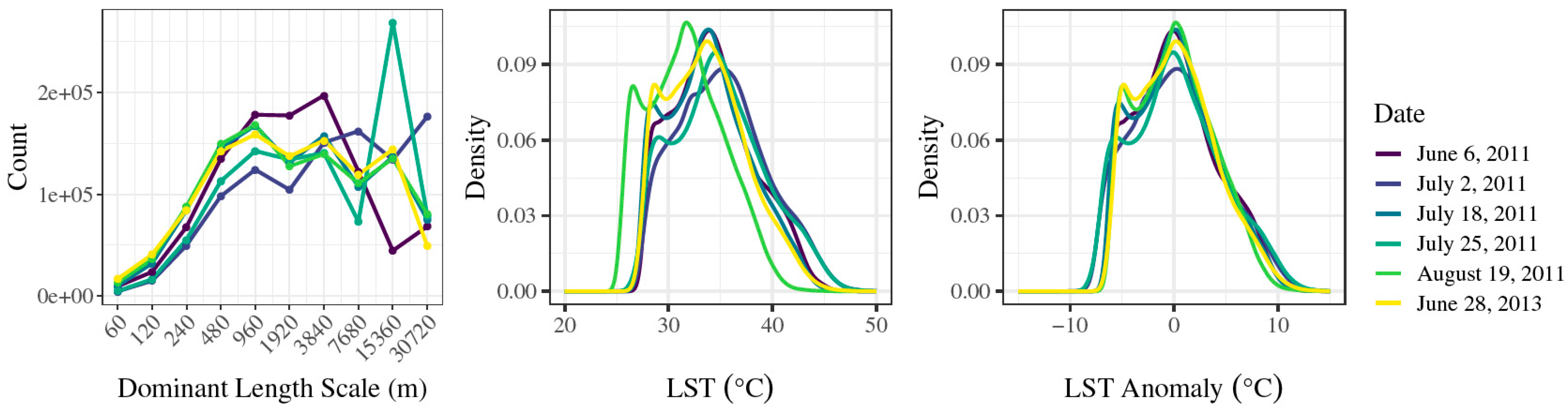
3.1. Variation of Dominant Length Scales and LST

We completed the multi-resolution wavelet analysis and subsequent metric calculations for a sample of 100 pixels of each dominant length scale for each of the six dates, for a total sample of 5400 pixels. The dominant length scales gave us the extent within which the metrics were calculated and represent the characteristic scales of the biophysical interactions that produce LST (Figure 3).
The dominant length scales followed approximately the same distribution for each date up to the 960 m scale. 28 June, 18 July, and 19 August, which were the coolest days on average, all peaked at this scale. June 6 peaks at the 3840 m scale followed by a sharp decrease, 2 July increased to a peak at 30,720 m, and 25 July had a strong peak at 15,360 m. 2 July and 25 July were also the warmest days on average (Figure 4).
LST anomalies followed approximately the same distribution for each date with 2 July and 25 July having more negative temperature anomalies (Figure 4).
LST anomalies varied only slightly by dominant length scale, with the mean anomaly increasing slightly at the 30,720 m scale and all other scales showing a mean LST anomaly of approximately zero (results not shown). This indicates that the strength of the LST anomaly does not depend on the extent of the area at which temperature is produced for a given pixel. All scales were positively skewed with more positive LST anomalies than negative, a finding consistent with the definition of the UHI effect and expected for a study area comprised primarily of urban land cover.
LST varies predictably with the percent of vegetation, with areas with a higher percentage of green space showing lower temperatures at any given scale (Figure 5).
It is worth noting that as scale increases, there were no observations in both the lowest and highest percent vegetated classes. The larger the area, the more likely it is that there will be some amount of green space and the less likely it is that the area will be entirely green space. This is also a consequence of the wavelet analysis—eventually the coarsest scale of an image decomposition will approach a constant value which is the mean of the unstandardized LST values. This indicates that the areas in the highest and lowest percent vegetated classes do not make significant contributions to mean LST.

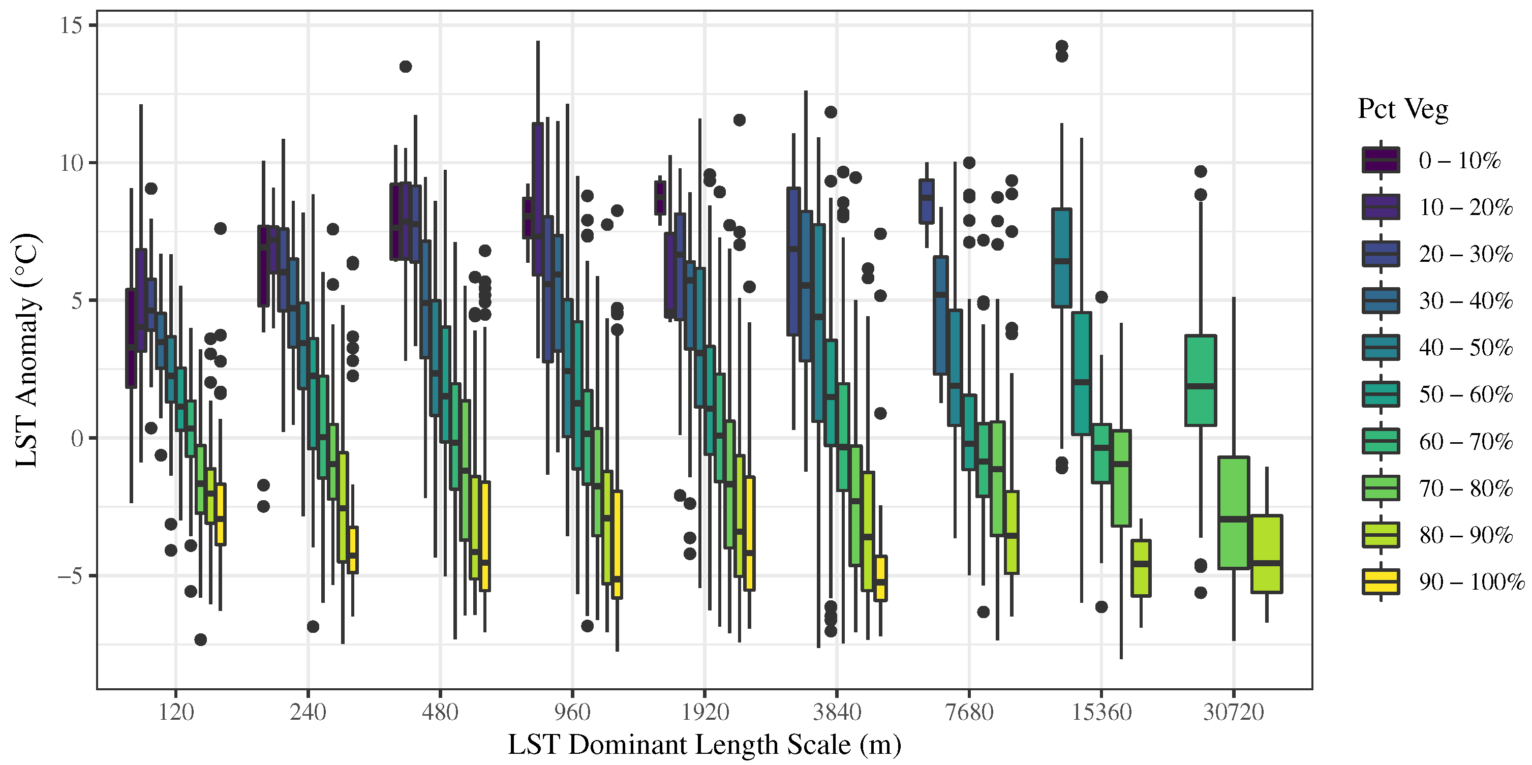
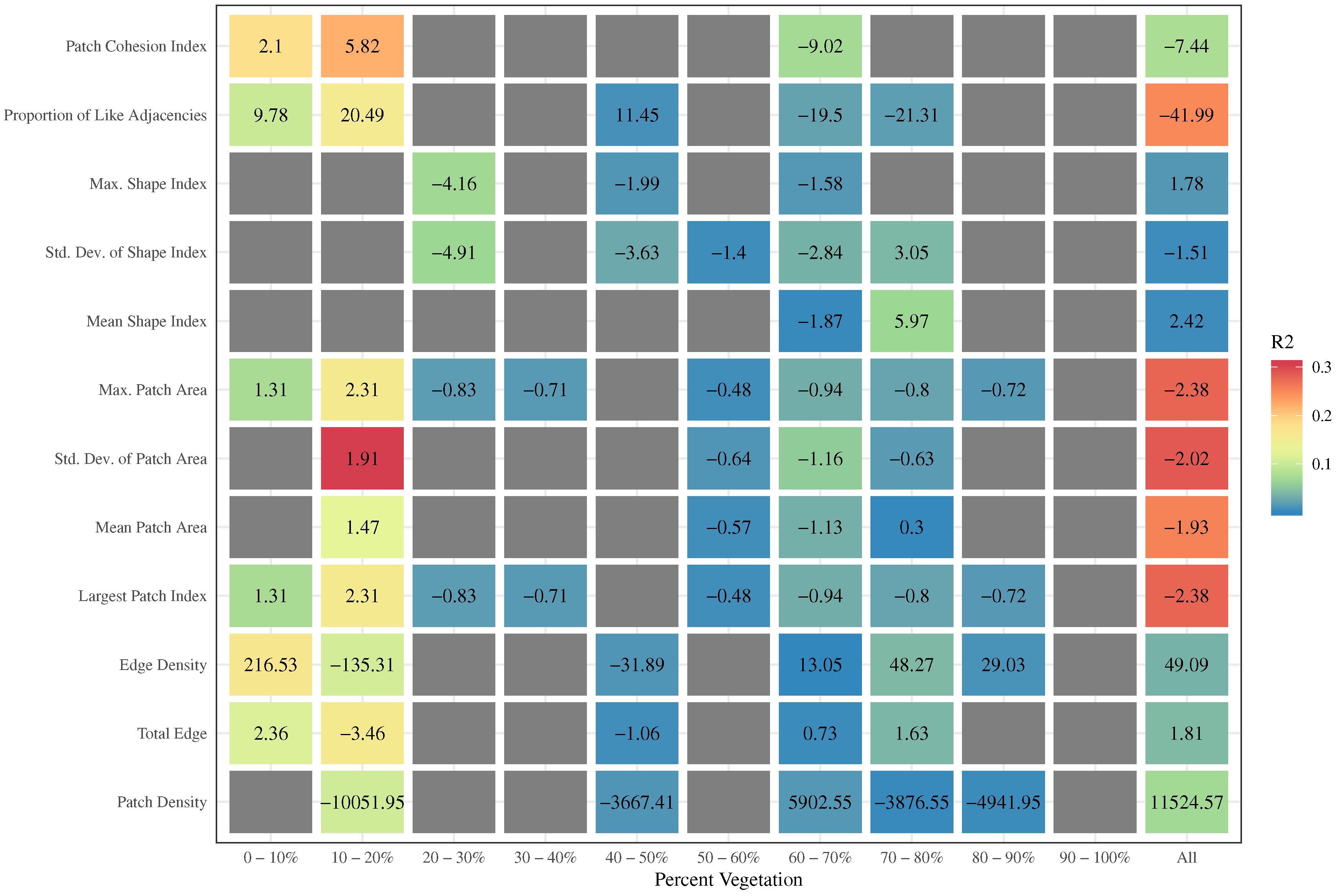
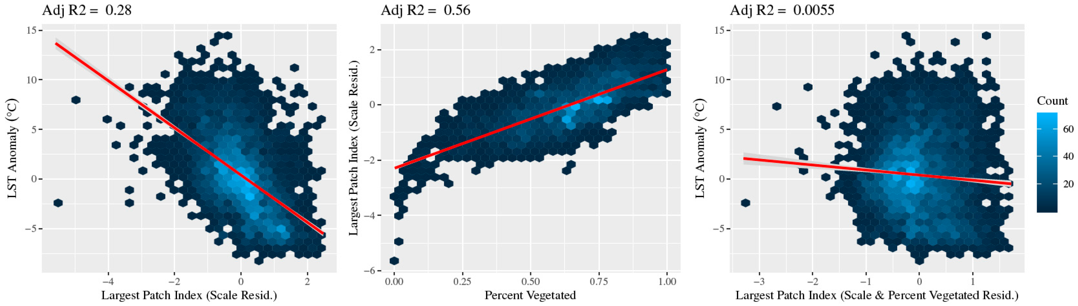
3.2. Relationship between Landscape Metrics and LST

All the metrics were significantly correlated with scale (Table 3).
This is part and parcel of the modifiable areal unit problem (MAUP) that plagues most geographic analysis and is the consequence of the dyadic increase in area of the calculation extent that accompanies an increase in dominant length scale. In order to compare metrics calculated at different dominant length scales and to remove these scaling effects, the residuals from the best fit linear regression models between LST and the landscape metrics were used in the analysis (Table 4).
Having removed the effects of increasing scale on the metric values we then examined the relationship between LST and the landscape metrics. The Pearson correlation coefficients show that all metrics are significantly correlated with LST.
However, all metrics are also significantly correlated with the percent of vegetation (Table 5). Following the work of Hu and Brunsell [57], the observations were broken into ten equal-interval classes according to the percent of vegetation to isolate the effects of landscape configuration on the SUHI. By regressing LST on the metric values within each percent vegetated class, we controlled for the effects of the correlation between the metrics and the percent of vegetation. After controlling for the percent of vegetation the relationships between the metrics and LST changed greatly.
Figure 6 compares the correlation coefficients for LST and the landscape metrics for each percent vegetated class to the correlation between LST and the metrics without controlling for the percent of vegetation. Many of the metrics show moderately strong correlations with LST for levels of percent vegetated cover less than 20%, however, the sign of these relationships are opposite to the sign of the remainder of the percent vegetated classes for nearly all of the metrics. Additionally, these metrics describe conflicting elements of landscape pattern, suggesting that for percent vegetated cover of less than 10%, both fragmentation and connectivity increase LST. None of the metrics show significant and consistent relationships with LST, with many changing direction multiple times between percent vegetated classes, indicating that green space configuration is not a reliable or robust moderator of the effect of increasing the amount of green space on LST.
Additionally, we regressed LST on each metric for each percent vegetated class.
Figure 7 shows how the slopes of the regression lines and the proportion of the variance of LST ( R 2 ) that is explained by the metrics vary across the percent vegetated classes. Only the colored cells have significant slope coefficients. While the slopes cannot be compared between the different landscape metrics, it is clear that the relationships between the metrics and LST change sign across the percent vegetated classes. The rightmost column shows the relationship between the metrics and LST without controlling for the percent of vegetation. While the proportion of like adjacencies, maximum patch area, the standard deviation of patch area, mean patch area, and largest patch index all approach an R 2 value of 0.3 without controlling for the percent of vegetation, when we examine these relationships within the percent vegetated classes, the R 2 values are much lower. In areas with less than 20% vegetation, the R 2 values range from 0.08 to 0.18 with the exception of the standard deviation of patch area which for the 10 to 20% vegetated class has an R 2 value of 0.31. However, the slope of this relationship is positive while other percent vegetated classes show negative relationships. For all classes between 20% and 100% vegetated, all metrics exhibit very low R 2 values, ranging from 0.002 to 0.072. This indicates that at most, the configuration of green space accounts for 7.2% of the variation in LST.
To provide a check on these results we regressed the metric values on the percent of vegetation and examined the residuals from these models plotted against LST. These residuals represent metric values that are uncorrelated with both calculation extent and the percent of vegetation. It is clear that there remains no relationship between landscape metrics and LST. For example, the relationship between the largest patch index and LST has an R 2 value of 0.28 but after controlling for the percent of vegetation this relationship diminishes to an R 2 of 0.0055 (Figure 8).

4. Discussion

4.1. Methodological Implications for Urban Landscape Pattern Analysis

It is our contention that pattern analysis should take place at the characteristic scale of vegetation–LST interaction and that comparing a pattern in variably sized extents, which are not biophysically relevant, fails to capture the complexity of urban energy interactions [6,33]. If the spatial distribution of LST is moderated and enhanced by the spatial distribution of green space then studies seeking to understand the nature of this relationship should quantify green space pattern within extents defined by the process scale of LST production. Landscape metrics are sensitive to the size and shape of the extent within which they are calculated and doing so within extents that are arbitrarily defined may produce spurious results [19]. Using irregularly-shaped extents like census blocks may produce metric values that are biased by the shape of the analytical extent itself. In this study, we calculated the dominant length scales of LST in Kansas City metropolitan area to analyze green space configuration within the scale at which biophysical interactions on the Earth’s surface produce LST. Wavelet analysis provides a robust means of determining relevant extents to analyze the relationship between LST and green space pattern. Our methodology also removes the need to aerially aggregate LST, a strategy which obscures some of the variability that studies of this nature seek to explain.
It is also important that a comparison of landscape pattern be either based on the same extent or done in a manner that explicitly addresses scale [35]. If landscape pattern is dependent on the spatial scale at which it is examined, it logically follows that landscape metrics calculated for different spatial scales may not be analogous unless the scaling effects are removed. In order to compare metrics calculated at different dominant length scales, we analyzed the residuals from the metric values regressed on calculation extent. Using the residuals rather than the unstandardized metric values provides a quantification of the green space pattern uncorrelated with the scaling effects. Thus, we maintain the information about the biophysical interactions that produce LST given by the identification of the dominant length scales while allowing comparison between them.
Additionally, it is clear from this and other studies [16,36] that controlling for the percent of vegetation is essential to the interpretation of metric values. Landscape metric values are strongly dependent on the abundance of the land cover type they are measuring. For example, as the percent of green space increases within an area, the size of the largest green space patch is likely to increase as well. If the correlations between the green space configuration metrics and the percent of vegetation are not accounted for explicitly, the apparent relationships between green space configurations and LST may be spurious. Without controlling for the percent of vegetation there appear to be moderately strong relationships between the patch size, fragmentation, connectivity, and proximity metrics but these relationships become very weak after removing the effects of the percent of vegetation. For areas with less than 20% vegetation, many of these relationships even change sign. For example, the correlations of both the largest patch index and the maximum patch area with LST are negative for above 20% vegetated, but this relationship is positive for the sparsely vegetated areas. By examining relationships between LST and landscape metrics across ten equal-interval percent vegetated classes we were able to isolate the effects of configuration on LST. While this is not a novel contribution of our study, it is important to highlight that while the percent of vegetation has a consistently negative effect on urban LST, green space pattern has at best weak, and often contradictory effects. For urban planners and municipalities seeking to mitigate SUHIs, increasing the amount of green space by planting vegetation wherever possible may be a simpler task than attempting to alter the existing built environment in order to influence green space pattern.

4.2. Percent of Vegetation Has a Consistent Negative Effect on LST, However the Contribution of the Spatial Configuration of Green Space Is Negligible

The percent of vegetation has a significant negative effect on LST regardless of the extent of analysis, with higher R 2 values for the 120 and 240 m extents (Table 6). This finding is corroborated by numerous other studies [16,17,27,36].
Green space lowers LST by transforming incoming solar radiation to latent heat through evapotranspiration and by providing shading, thereby reducing the release of sensible heat. Increasing the percent of green space can effectively lower LST in the Kansas City metropolitan area.
The landscape metrics used in this study describe five elements of configuration: patch size, fragmentation, shape, connectivity, and proximity. After controlling for both the resolution of the calculation extent and the percent of vegetation, the effects of green space configuration on LST were negligible and inconsistent. Examining the relationship between metrics and LST across ten equal-interval percent vegetated classes showed that, while the proportion of like adjacencies, maximum patch area, the standard deviation, mean, and maximum patch area, and the largest patch index account for almost 30% of the variability in LST, this explanatory power is primarily due to the correlation between these metrics and the percent of vegetation (Figure 7). Edge density, largest patch index, maximum patch area, mean patch area, patch cohesion index, the proportion of like adjacencies, standard deviation of the patch area and total edge all have significant and positive relationships with LST in areas less than 20% vegetated, indicating that as these metric values increase, so does temperature in sparsely vegetated areas. However, these metrics describe the conflicting attributes of patch size, fragmentation, connectivity, and proximity. While an interpretation of these results might suggest that for low vegetation areas an evenly distributed configuration of green space may lower LST, the more insightful interpretation is that simply increasing the amount of green space regardless of configuration will lower LST. Likewise, in Figure 6 it is tempting to see trends in the 20 to 90% vegetated levels, however, it is important to remember that these relationships explain a maximum of 7% of the variability in LST. Again, a more insightful interpretation is that altering specific configurations, i.e., increasing the maximum patch area or decreasing edge density would do very little to increase the cooling power of green space beyond the effects of increasing the percent of vegetation. Although Li et al. [28] found that the configuration of green space was more important than the percent of vegetation in lowering LST, their analytical extents were census tracts whose boundaries have little to do with the biophysical interactions that produce temperature.
Urban planning is a complex process requiring the cooperation of multiple agencies and stakeholder groups and the allocation of limited resources. Greenspace management options require the implementation of policy tools which must be approved by local governments and are constrained by federal and state regulations [58]. Additionally, urban ecosystems are comprised of not only biological and physical systems but also social ones. These human and natural processes interact to produce uneven landscapes of vulnerability [59] and research seeking to inform planners in land-use decisions regarding urban heat must consider the difficulty with which change is affected. The simple answer that increasing green space can lower LST regardless of configuration allows the prioritization of resources towards benefiting neighborhoods most vulnerable to the impacts of UHIs.

4.3. Limitations

While this study does provide a methodology for robust biophysically-based analysis of urban landscape pattern and demonstrates that the contributions of green space configuration to the SUHI are negligible in Kansas City metropolitan area, there are limitations to the interpretation of our results. Firstly, our research considered only one city; it would be a valuable contribution to extend these methods to multiple urban areas in order to explore the generalizability of our conclusions. Secondly, although log transformation placed many of the relationships between metrics and scale in the linear domain, modeling these relationships as nonlinear may explain some of the remaining variations in the metric values and warrants further investigation. While thermal remote sensing is a valuable approach to modeling SUHIs, it results in the spatial averaging of LST in a way that may obscure the small-scale variation of urban temperature and the importance of the urban canopy. Future work by the authors will extend this research to incorporate high-resolution urban climate simulations that model air temperature in addition to LST. Finally, results from the analysis of remotely sensed images are inherently dependent on image resolution. Although higher-resolution LST data would allow the detection of finer dominant length scales, we expect that this scale of variability would not be the dominant scale of the surface energy balance and LST in a significant number of areas [60]. This would, of course, depend upon the morphology of the city under consideration.

5. Conclusions

Urban green space is a significant mitigating factor in the formation of surface urban heat islands. It is well understood that increasing the amount of green space has a cooling effect on urban temperatures but studies on the effects of the pattern of green space have produced inconsistent and sometimes contradictory results [16,17,22,24,27,28,29]. Furthermore, these studies have analyzed pattern within extents that are not defined by the biophysical interactions that produce LST [17,22,24,27,28,29,31]. To investigate the relationship between green space configuration and LST in the Kansas City metropolitan area, we conducted a wavelet analysis to determine the dominant length scales of LST production in order to ensure that our quantification of landscape pattern was not arbitrarily constrained but instead formed by the energetic flows of the landscape itself. Additionally, we controlled for both the size of the calculation extents and the percent of vegetation. Our findings indicate that green space configuration has comparatively little effect on the SUHI and that the cooling effects of vegetation are due primarily to the percent of green space in an urban area rather than its pattern. Future research should focus on extending these methods temporally, as well as to other urban areas characterized by different climates.
UHI abatement is a powerful strategy to both reduce heat stress and adapt to climate change and urban planning has the potential to increase the resilience of urban areas through improvements to the built environment and green infrastructure. Our results have powerful implications for urban planners: more green space is better green space, regardless of the configuration. Green infrastructure planning need not be constrained by considerations of configuration and complex quantifications and statistical analyses are unnecessary for scenario planning. Instead, resources can be focused on social and environmental justice and public health outcomes regarding green infrastructure.

Author Contributions

Conceptualization, E.J.W.; Formal analysis, E.J.W.; Funding acquisition, N.A.B.; Methodology, E.J.W. and N.A.B.; Project administration, N.A.B.; Writing—original draft, E.J.W.; Writing—review and editing, E.J.W. and N.A.B.

Funding

This work was funded through the National Science Foundation (NSF0069549).

Conflicts of Interest

The authors declare no conflict of interest.

References

  1. United Nations. World Urbanization Prospects: The 2014 Revision; Technical Report; United Nations, Department of Economic and Social Affairs, Population Division: New York, NY, USA, 2014. [Google Scholar]
  2. Akbari, H.; Pomerantz, M.; Taha, H. Cool surfaces and shade trees to reduce energy use and improve air quality in urban areas. Sol. Energy 2001, 70, 295–310. [Google Scholar] [CrossRef]
  3. Voogt, J.A.; Oke, T.R. Thermal remote sensing of urban climates. Remote Sens. Environ. 2003, 86, 370–384. [Google Scholar] [CrossRef]
  4. Alberti, M. Maintaining ecological integrity and sustaining ecosystem function in urban areas. Curr. Opin. Environ. Sustain. 2010, 2, 178–184. [Google Scholar] [CrossRef]
  5. Oke, T.R. The Heat Island of the Urban Boundary Layer: Characteristics, Causes and Effects. In Wind Climate in Cities of NATO ASI Series; Cermak, J.E., Davenport, A.G., Plate, E.J., Viegas, D.X., Eds.; Springer: Dordrecht, The Netherlands, 1995; Volume 277, pp. 81–107. [Google Scholar] [CrossRef]
  6. Weng, Q.H.; Liu, H.; Liang, B.Q.; Lu, D.S. The spatial variations of urban land surface temperatures: Pertinent factors, zoning effect, and seasonal variability. IEEE J. Sel. Top. Appl. Earth Obs. Remote Sens. 2008, 1, 154–166. [Google Scholar] [CrossRef]
  7. Weng, Q.; Lu, D.; Schubring, J. Estimation of land surface temperature-vegetation abundance relationship for urban heat island studies. Remote Sens. Environ. 2004, 89, 467–483. [Google Scholar] [CrossRef]
  8. Imhoff, M.L.; Zhang, P.; Wolfe, R.E.; Bounoua, L. Remote sensing of the urban heat island effect across biomes in the continental USA. Remote Sens. Environ. 2010, 114, 504–513. [Google Scholar] [CrossRef] [Green Version]
  9. Grimmond, C.S.B.; Oke, T.R. An evapotranspiration-interception model for urban areas. Water Resour. Res. 1991, 27, 1739–1755. [Google Scholar] [CrossRef]
  10. Hu, L.; Brunsell, N.A. The impact of temporal aggregation of land surface temperature data for surface urban heat island (SUHI) monitoring. Remote Sens. Environ. 2013, 134, 162–174. [Google Scholar] [CrossRef]
  11. Stone, B.; Vargo, J.; Habeeb, D. Managing climate change in cities: Will climate action plans work? Landsc. Urban Plan. 2012, 107, 263–271. [Google Scholar] [CrossRef]
  12. Meehl, G.A.; Tebaldi, C. More intense, more frequent, and longer lasting heat waves in the 21st century. Science 2004, 305, 994–997. [Google Scholar] [CrossRef]
  13. Luber, G.; McGeehin, M. Climate change and extreme heat events. Am. J. Prev. Med. 2008, 35, 429–435. [Google Scholar] [CrossRef] [PubMed]
  14. Patz, J.A.; Campbell-Lendrum, D.; Holloway, T.; Foley, J.A. Impact of regional climate change on human health. Nature 2005, 438, 310–317. [Google Scholar] [CrossRef] [PubMed]
  15. Stott, P.A.; Stone, D.A.; Allen, M.R. Human contribution to the European heatwave of 2003. Nature 2004, 432, 610–614. [Google Scholar] [CrossRef] [PubMed]
  16. Zhou, W.; Huang, G.; Cadenasso, M.L. Does spatial configuration matter? Understanding the effects of land cover pattern on land surface temperature in urban landscapes. Landsc. Urban Plan. 2011, 102, 54–63. [Google Scholar] [CrossRef]
  17. Maimaitiyiming, M.; Ghulam, A.; Tiyip, T.; Pla, F.; Latorre-Carmona, P.; Halik, Ü.; Sawut, M.; Caetano, M. Effects of green space spatial pattern on land surface temperature: Implications for sustainable urban planning and climate change adaptation. ISPRS J. Photogramm. Remote Sens. 2014, 89, 59–66. [Google Scholar] [CrossRef] [Green Version]
  18. Weng, Q.; Liu, H.; Lu, D. Assessing the effects of land use and land cover patterns on thermal conditions using landscape metrics in city of Indianapolis, United States. Urban Ecosyst. 2007, 10, 203–219. [Google Scholar] [CrossRef]
  19. McGarigal, K. FRAGSTATS Help. 2015. Available online: https://www.umass.edu/landeco/research/fragstats/documents/fragstats.help.4.2.pdf (accessed on 10 August 2019).
  20. Huang, G.; Zhou, W.; Cadenasso, M.L. Is everyone hot in the city? Spatial pattern of land surface temperatures, land cover and neighborhood socioeconomic characteristics in Baltimore, MD. J. Environ. Manag. 2011, 92, 1753–1759. [Google Scholar] [CrossRef]
  21. Buyantuyev, A.; Wu, J. Urban heat islands and landscape heterogeneity: Linking spatiotemporal variations in surface temperatures to land-cover and socioeconomic patterns. Landsc. Ecol. 2010, 25, 17–33. [Google Scholar] [CrossRef]
  22. Li, J.; Song, C.; Cao, L.; Zhu, F.; Meng, X.; Wu, J. Impacts of landscape structure on surface urban heat islands: A case study of Shanghai, China. Remote Sens. Environ. 2011, 115, 3249–3263. [Google Scholar] [CrossRef]
  23. Yuan, F.; Bauer, M.E. Comparison of impervious surface area and normalized difference vegetation index as indicators of surface urban heat island effects in Landsat imagery. Remote Sens. Environ. 2007, 106, 375–386. [Google Scholar] [CrossRef]
  24. Chen, Y.; Yu, S. Impacts of urban landscape patterns on urban thermal variations in Guangzhou, China. Int. J. Appl. Earth Obs. Geoinf. 2017, 54, 65–71. [Google Scholar] [CrossRef]
  25. Wu, J. Urban sustainability: An inevitable goal of landscape research. Landsc. Ecol. 2010, 25, 1–4. [Google Scholar] [CrossRef]
  26. Leitao, A.B.; Ahern, J. Applying landscape ecological concepts and metrics in sustainable landscape planning. Landsc. Urban Plan. 2002, 59, 65–93. [Google Scholar] [CrossRef]
  27. Li, X.; Zhou, W.; Ouyang, Z.; Xu, W.; Zheng, H. Spatial pattern of greenspace affects land surface temperature: Evidence from the heavily urbanized Beijing metropolitan area, China. Landsc. Ecol. 2012, 27, 887–898. [Google Scholar] [CrossRef]
  28. Li, X.; Li, W.; Middel, A.; Harlan, S.L.; Brazel, A.J.; Turner, B.L., II. Remote sensing of the surface urban heat island and land architecture in Phoenix, Arizona: Combined effects of land composition and configuration and cadastral-demographic-economic factors. Remote Sens. Environ. 2016, 174, 233–243. [Google Scholar] [CrossRef]
  29. Estoque, R.C.; Murayama, Y.; Myint, S.W. Effects of landscape composition and pattern on land surface temperature: An urban heat island study in the megacities of Southeast Asia. Sci. Total Environ. 2017, 577, 349–359. [Google Scholar] [CrossRef] [PubMed]
  30. Stone, B.; Rodgers, M.O. Urban form and thermal efficiency: How the design of cities influences the urban heat island effect. J. Am. Plan. Assoc. 2001, 67, 186–198. [Google Scholar] [CrossRef]
  31. Grafius, D.R.; Corstanje, R.; Harris, J.A. Linking ecosystem services, urban form and green space configuration using multivariate landscape metric analysis. Landsc. Ecol. 2018, 33, 1–17. [Google Scholar] [CrossRef]
  32. Liu, J.; Dietz, T.; Carpenter, S.R.; Alberti, M.; Folke, C.; Moran, E.; Pell, A.N.; Deadman, P.; Kratz, T.; Lubchenco, J.; et al. Complexity of Coupled Human and Natural Systems. Science 2007, 317, 1513–1516. [Google Scholar] [CrossRef] [Green Version]
  33. Wu, J. Scale and Scaling: A Cross-Disciplinary Perspective. In Key Topics in Landscape Ecology; Cambridge University Press: Cambridge, UK, 2007; pp. 115–142. [Google Scholar]
  34. Wu, J. Key concepts and research topics in landscape ecology revisited: 30 years after the Allerton Park workshop. Landsc. Ecol. 2013, 28, 1–11. [Google Scholar] [CrossRef]
  35. Wu, J. Effects of changing scale on landscape pattern analysis: Scaling relations. Landsc. Ecol. 2004, 19, 125–138. [Google Scholar] [CrossRef]
  36. Zhou, W.; Wang, J.; Cadenasso, M.L. Effects of the spatial configuration of trees on urban heat mitigation: A comparative study. Remote Sens. Environ. 2017, 195, 1–12. [Google Scholar] [CrossRef]
  37. Guo, G.; Wu, Z.; Chen, Y. Complex mechanisms linking land surface temperature to greenspace spatial patterns: Evidence from four southeastern Chinese cities. Sci. Total Environ. 2019, 674, 77–87. [Google Scholar] [CrossRef] [PubMed]
  38. Buyantuyev, A.; Wu, J.; Gries, C. Multiscale analysis of the urbanization pattern of the Phoenix metropolitan landscape of USA: Time, space and thematic resolution. Landsc. Urban Plan. 2010, 94, 206–217. [Google Scholar] [CrossRef]
  39. Kumar, P.; Foufoula-Georgiou, E. Wavelet analysis for geophysical applications. Rev. Geophys. 1997, 35, 385–412. [Google Scholar] [CrossRef] [Green Version]
  40. Brunsell, N.A.; Gillies, R.R. Length scale analysis of surface energy fluxes derived from remote sensing. J. Hydrometeorol. 2003, 4, 1212–1219. [Google Scholar] [CrossRef]
  41. R Core Team. R: A Language and Environment for Statistical Computing; R Foundation for Statistical Computing: Vienna, Austria, 2018. [Google Scholar]
  42. Kottek, M.; Grieser, J.; Beck, C.; Rudolf, B.; Rubel, F. World map of the Köppen-Geiger climate classification updated. Meteorol. Z. 2006, 15, 259–263. [Google Scholar] [CrossRef]
  43. Stone, B.; Hess, J.J.; Frumkin, H. Urban form and extreme heat events: Are sprawling cities more vulnerable to climate change than compact cities? Environ. Health Perspect. 2010, 118, 1425–1428. [Google Scholar] [CrossRef]
  44. Ji, W. Landscape effects of urban sprawl: Spatial and temporal analyses using remote sensing images and landscape metrics. Int. Arch. Photogramm. Remote Sens. Spat. Inf. Sci. 2008, 37, 1691–1694. [Google Scholar]
  45. Stone, B.; Norman, J.M. Land use planning and surface heat island formation: A parcel-based radiation flux approach. Atmos. Environ. 2006, 40, 3561–3573. [Google Scholar] [CrossRef]
  46. Liu, H.; Weng, Q. Scaling effect on the relationship between landscape pattern and land surface temperature: A case study of Indianapolis, United States. Photogramm. Eng. Remote Sens. 2009, 75, 291–304. [Google Scholar] [CrossRef]
  47. Li, X.; Zhou, W.; Ouyang, Z. Relationship between land surface temperature and spatial pattern of greenspace: What are the effects of spatial resolution? Landsc. Urban Plan. 2013, 114, 1–8. [Google Scholar] [CrossRef]
  48. Mid-America Regional Council; Applied Ecological Services. Kansas City Natural Resource Inventory II: Beyond the Map Summary Report; Technical Report; Mid-America Regional Council: Kansas City, MO, USA, 2013. [Google Scholar]
  49. Gillies, R.R.; Carlson, T.N. Thermal remote sensing of surface soil water content with partial vegetation cover for incorporation into climate models. J. Appl. Meteorol. 1995, 34, 745–756. [Google Scholar] [CrossRef]
  50. Carlson, T.N.; Ripley, D.A. On the relation between NDVI, fractional vegetation cover, and leaf area index. Remote Sens. Environ. 1997, 62, 241–252. [Google Scholar] [CrossRef]
  51. Brunsell, N.A.; Gillies, R.R. Incorporating surface emissivity into a thermal atmospheric correction. Photogramm. Eng. Remote Sens. 2002, 68, 1263–1269. [Google Scholar]
  52. Xu, H. Modification of normalised difference water index (NDWI) to enhance open water features in remotely sensed imagery. Int. J. Remote Sens. 2006, 27, 3025–3033. [Google Scholar] [CrossRef]
  53. U.S. Geological Survey. Landsat 8 (L8) Data Users Handbook, Version 3.0. Available online: https://www.usgs.gov/media/files/landsat-8-data-users-handbook (accessed on 7 June 2019).
  54. Zhou, Y.; Smith, S.J.; Elvidge, C.D.; Zhao, K.; Thomson, A.; Imhoff, M. A cluster-based method to map urban area from DMSP/OLS nightlights. Remote Sens. Environ. 2014, 147, 173–185. [Google Scholar] [CrossRef]
  55. Whitcher, B. Waveslim: Basic Wavelet Routines for One-, Two- and Three-Dimensional Signal Processing. 2015. Available online: https://cran.r-project.org/package=waveslim (accessed on 7 June 2019).
  56. Evans, J.S.; spatialEco. R Package Version 0.1.1-1. Available online: https://github.com/jeffreyevans/spatialEco (accessed on 7 June 2019).
  57. Hu, L.; Brunsell, N.A. A new perspective to assess the urban heat island through remotely sensed atmospheric profiles. Remote Sens. Environ. 2015, 158, 393–406. [Google Scholar] [CrossRef]
  58. Hoverter, S.P. Adapting to Urban Heat: A Tool Kit for Local Governments; Technical Report; Georgetown Climate Center: Washington, DC, USA, 2012. [Google Scholar]
  59. Cadenasso, M.L.; Pickett, S.T.A. Urban principles for ecological landscape design and management: Scientific fundamentals. Urban Ecol. 2008, 1, 1–16. [Google Scholar]
  60. Schmid, H.; Cleugh, H.; Grimmond, C.; Oke, T. Spatial variability of energy fluxes in suburban terrain. Bound. Lay. Meteorol. 1991, 54, 249–276. [Google Scholar] [CrossRef] [Green Version]
Figure 1. The Kansas City metropolitan area (left)—shown as a false color composite Landsat image from 6 June 2011—exhibits characteristic patterns of urban sprawl. The spatial distribution of green space (right) with green pixels representing green space and grey pixels representing all non-vegetated surfaces. The location of Kansas City within the U.S. is also shown.
Remotesensing 11 02322 g001
Figure 2. Ten-level wavelet decomposition (right) of the land surface temperature (LST) image from 25 July 2011 (left). The levels of decomposition show the contribution of each pixel to LST variability at each scale. The level one 60 m decomposition was discarded from the subsequent analysis.
Remotesensing 11 02322 g002
Figure 3. The dominant length scales (right) calculated from LST (left) for 25 July 2011. The dominant length scales represent the characteristic scales of the biophysical interactions that produce LST.
Remotesensing 11 02322 g003
Figure 4. Distribution of dominant length scales (left), LST (middle), and LST anomalies (right) by date.
Remotesensing 11 02322 g004
Figure 5. Boxplots showing the interquartile range of LST by the percent of vegetation and the dominant length scales. The bar in each box shows the median and the dots indicate outliers. LST varies only slightly by dominant length scale and decreases as the percent of vegetation increases, regardless of the dominant length scale.
Remotesensing 11 02322 g005
Figure 6. Correlations between metrics and LST by percent vegetated class. The dotted line indicates where the correlation changes sign and the colored line shows the correlation between metrics and LST without controlling for the percent of vegetation. Large significance symbols indicate r 0 . 2 .
Remotesensing 11 02322 g006
Figure 7. LST regressed on the metrics for each percent vegetated class. The numbers are the slope coefficient for models significant at p 0 . 05 and the color indicates the R 2 value of the regression models. The rightmost column is LST regressed on the metrics without controlling for the percent of vegetation.
Remotesensing 11 02322 g007
Figure 8. LST plotted against the largest patch index without controlling for the percent of vegetation (left) and after controlling for the percent of vegetation (right). The middle plot shows the relationship between the largest patch index and the percent of vegetation that accounts for most of the influence of the largest patch index on LST.
Remotesensing 11 02322 g008
Table 1. Satellite acquisition dates and sensors.
DateSensor
7 June 2011Landsat 5
2 July 2011Landsat 5
18 July 2011Landsat 5
25 July 2011Landsat 5
19 August 2011Landsat 5
28 June 2013Landsat 7
Table 2. Landscape metrics calculated to quantify landscape pattern. Composition is quantified by the proportion of landscape while configuration is quantified by the patch size, fragmentation, shape, connectivity, and proximity metrics. For a more in-depth explanation of landscape metrics see McGarigal [19].
Pattern MeasureLandscape MetricDescriptionEquation
CompositionProportion of landscape (PLAND)Percent of landscape composed of vegetated surfaces. j = 1 n i a i j A ( 100 )
Patch sizePatch size distribution (AREA)The statistical distribution of vegetated patch sizes, including the mean, minimum, maximum, and standard deviation. A R E A = a i j
FragmentationLargest patch index (LPI)Percentage of each dominant length scale extent comprised of the largest vegetated patch. m a x j = 1 n ( a i j ) A ( 100 )
Patch density (PD)Number of vegetated patches divided by the area of the extent. n i A
Total edge (TE)Total perimeter length of all vegetated patches within an extent. k = 1 m e i k
Edge density (ED)Total perimeter length of all vegetated patches within an extent divided by the area of that extent. k = 1 m e i k A
ShapeShape index distribution (SHAPE)Statistical distribution of the shape index which provides a standardized measure of shape complexity calculated from the perimeters of the vegetated patches within each extent. A measure of disaggregation. P i j m i n P i j
ConnectivityPatch cohesion index (COHESION)Measure of the physical connectedness of the vegetated patches within each dominant length scale extent which increases as patches become more aggregated. 1 j = 1 n P i j j = 1 n P i j a i j 1 1 A 1 ( 100 )
ProximityProportion of like adjacencies (PLADJ)Degree of aggregation of vegetated patches. g i j k = 1 m g i k ( 100 )
n i is the number of vegetated patches, a i j is the area ( m 2 ) of patch a i j , A is the total area ( m 2 ) of the extent, m a x j = 1 n ( a i j ) is the max. patch size within the extent, n i is the number of vegetated patches within the extent, e i k is the total perimeter length of the vegetated patches, P i j is the perimeter of patch i j , m i n P i j is the min. vegetated patch perimeter, g i j is the number of like adjacencies to vegetated pixel i j , and g i k is the total number of adjacencies of vegetated pixels within the extent.
Table 3. Pearson’s correlation coefficients for metrics by the log of the dominant length scales. Some metric values have been log transformed according to the best fit models.
Metric Scale
Prop. of Landscape0.15
Patch Density−0.44
Total Edge0.99
Edge Density−0.36
Largest Patch Index−0.80
Mean Patch Area0.31
Std. Dev. of Patch Area0.73
Max. Patch Area0.94
Mean Shape Index0.33
Std. Dev. of Shape Index0.66
Max. Shape Index0.94
Prop. of Like Adjacencies0.37
Patch Cohesion Index0.71
All values are significant at p < 0 . 001 .
Table 4. Best fit models for metric (y) by dominant length scale (x).
MetricModel R 2
Patch Densityy log(x)0.19
Total Edgelog(y) log(x)0.98
Edge Densityy log(x)0.13
Largest Patch Indexlog(y) log(x)0.64
Mean Patch Arealog(y) log(x)0.10
Std. Dev. of Patch Arealog(y) log(x)0.53
Max. Patch Arealog(y) log(x)0.88
Mean Shape Indexlog(y) log(x)0.11
Std. Dev. of Shape Indexy log(x)0.43
Max. Shape Indexlog(y) log(x)0.88
Proportion of Like Adjacenciesy log(x)0.13
Patch Cohesion Indexy log(x)0.51
Table 5. Pearson’s correlation coefficients for LST regressed on metric values and for metrics regressed on the percent of vegetation. All metrics were significantly correlated with LST but also with the percent of vegetation.
LST MetricMetric Pct Veg
Patch Density0.26−0.44
Total Edge0.21−0.24
Edge Density0.19−0.22
Largest Patch Index−0.530.75
Mean Patch Area−0.500.80
Std. Dev. of Patch Area−0.540.77
Max. Patch Area−0.530.75
Mean Shape Index0.08−0.08
Std. Dev. of Shape Index−0.080.08
Max. Shape Index0.12−0.26
Proportion of Like Adjacencies−0.500.80
Patch Cohesion Index−0.280.49
All values are significant at p < 0 . 001 .
Table 6. The percent of vegetation has a significant negative relationship with LST at all analytical extents. The results are the correlation coefficients between LST and the percent of vegetation for each dominant length scale (calculation extent).
ScaleLST Pct. Veg
120−0.76
240−0.75
480−0.70
960−0.66
1920−0.61
3840−0.66
7680−0.57
15360−0.65
30720−0.67
All values are significant at p < 0 . 001 .

