Abstract
Reference of Earth-observing satellite sensor data to a common, consistent radiometric scale is an increasingly critical issue as more of these sensors are launched; such consistency can be achieved through radiometric cross-calibration of the sensors. A common cross-calibration approach uses a small set of regions of interest (ROIs) in established Pseudo-Invariant Calibration Sites (PICS) mainly located throughout North Africa. The number of available cloud-free coincident scene pairs available for these regions limits the usefulness of this approach; furthermore, the temporal stability of most regions throughout North Africa is not known, and limited hyperspectral information exists for these regions. As a result, it takes more time to construct an appropriate cross-calibration dataset. In a previous work, Shrestha et al. presented an analysis identifying 19 distinct “clusters” of spectrally similar surface cover that are widely distributed across North Africa, with the potential to provide near-daily cloud-free imaging for most sensors. This paper proposes a technique to generate a representative hyperspectral profile for these clusters. The technique was used to generate the profile for the cluster containing the largest number of aggregated pixels. The resulting profile was found to have temporal uncertainties within 5% across all the spectral regions. Overall, this technique shows great potential for generation of representative hyperspectral profiles for any North African cluster, which could allow the use of the entire North Africa Saharan region as an extended PICS (EPICS) dataset for sensor cross-calibration. This should result in the increased temporal resolution of cross-calibration datasets and should help to achieve a cross-calibration quality similar to that of individual PICS in a significantly shorter time interval. It also facilitates the development of an EPICS based absolute calibration model, which can improve the accuracy and consistency in simulating any sensor’s top of atmosphere (TOA) reflectance.
1. Introduction
Satellite image data have been successfully used to characterize and monitor natural and man-made changes to the Earth’s surface over time. As the use of these sensors increases, a primary concern for researchers is ensuring the data are referenced to a common and consistent radiometric scale [1]. This can be achieved through accurate radiometric calibration of each sensor prior to its launch and at regular intervals after launch throughout its operating lifetime.
Many sensor designs include an onboard calibration data source such as lamps or a solar diffuser panel. For sensors without an onboard source, it may be possible to image the moon and generate a calibration dataset from these images. Alternatively, various calibration target regions on the Earth’s surface have “ground truth” radiance and/or reflectance measurements available during periods around a sensor overpass, allowing a more direct vicarious calibration approach. An indirect vicarious calibration approach involves cross-calibration between multiple sensors based on analysis of cloud-free coincident or near-coincident image pairs.
Cross-calibration is a post-launch calibration technique that uses a well-calibrated sensor as a transfer radiometer to achieve the radiometric calibration of an uncalibrated sensor using coincident and near coincident scenes of the Earth’s surface acquired by both sensors [1] and along with that it is also used to validate the in-orbit calibrated radiance. A transfer radiometer is radiometer that acts as an intermediate sensor to transfer the calibration of the well calibrated sensor to the uncalibrated sensor. Accurate cross-calibration places data from multiple sensors on a common, consistent radiometric scale [1,2] tied to a specific on-orbit calibration reference. It provides an alternative, cost-effective calibration method when (i) a sensor does not possess an onboard calibration system; and/or (ii) opportunities for vicarious calibration using surface radiance or reflectance measurements are limited or non-existent. Cross-calibration includes direct cross-calibration and indirect cross-calibration. The direct cross-calibration is the direction inter-calibration between two instruments, including the Simultaneous Nadir Overpass (SNO) and ray-matching methods. While in-direct cross-calibration needs a calibrated reference source (e.g., stable target) to inter-calibrate the two sensors. This paper is focused on the method for the in-direct cross-calibration using the deserts as the transfer.
1.1. Limitation of Region of Interest (ROI) Based Cross-Calibration Approach
Sensor cross-calibration is typically performed at a few Pseudo-Invariant Calibration Sites (PICS), located throughout the Sahara Desert in North Africa, where there is sufficient information available about the regional surface stability and a representative hyperspectral profile has been obtained. Depending on cloud cover at the site during each overpass and the revisit period of the sensor (e.g., 16 days for the Landsat sensors), several years are needed to construct a useful dataset for performing cross-calibration of optical satellite sensors and developing absolute calibration model. An absolute calibration model is a simple data-driven model which can simulate the TOA reflectance of virtually any optical sensor and is used for absolute calibration [3].
1.2. Proposed Solution to the ROI Based Cross-Calibration Approach
A representative hyperspectral profile of the site is crucial for developing spectral band adjustment factors (SBAFs) to account for differences in relative spectral response between sensors [1,4]. In a previous work, Shrestha et al. [5] identified an “extended” PICS (EPICS), widely spread across North Africa, that could be imaged on a near daily basis by any sensor as shown in Figure 1. These EPICS or clusters are the contiguous homogeneous regions which are spectrally similarly each other. Despite of its large spatial extent across North Africa, it behaves as a point site. Shrestha’s work indicated sufficient temporal and spatial stability to be considered as a candidate cross-calibration data source. However, it did not address determination of a representative hyperspectral profile from which the appropriate sensor SBAFs could be derived, thus limiting its suitability for cross-calibration work.
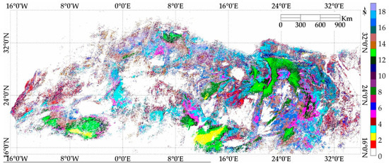
Figure 1.
K-Means Classification of North Africa to 5% Spatial Uncertainty.
This paper proposes an approach for generating a representative hyperspectral profile applicable to the set of surface characteristic “clusters” previously identified by Shrestha, mainly focusing on transmission regions of electromagnetic spectrum. The Earth Observer 1 (EO-1) Hyperion provides the image data used to generate the profiles; a brief overview of this sensor is provided in the Section 1.4. In principle, once a cluster’s representative hyperspectral profile has been generated, any region within the cluster can be used to cross-calibrate a sensor pair. Similarly, with the availability of a representative hyperspectral profile of an EPICS, they can also be used for the development of an absolute calibration model which will be briefly mentioned in Section 1.3. In a future paper, a cluster-based cross-calibration method is proposed that will significantly increase the temporal resolution of calibration time series datasets, which will help to achieve similar cross-calibration quality in a much shorter period of time compared to an individual PICS. Similarly, EPICS based absolute calibration model will also be developed which can provide a daily calibration point for any sensor.
1.3. EPICS Based Absolute Calibration Model
Helder et al. [3] developed a simple empirical absolute calibration model using Libya 4 observations by Terra MODIS and EO-1 Hyperion. In this model, Terra MODIS was used as the calibrated radiometer, whereas EO-1 Hyperion provided the target hyperspectral profile. Hyperspectral profile of the target is scaled to “match” the calibration of the sensor. When this scaled hyperspectral profile is integrated over the sensor relative spectral response (RSR), it will produce the comparable TOA reflectance of the specific sensor. The model was validated using corresponding Landsat 7 Enhanced Thematic Mapper (ETM+) observations and finding agreement of approximately 6% root mean square error (RMSE) between the sensor measured and modeled TOA reflectances, with approximately 2% random uncertainty. This TOA reflectance is compared to the observed TOA reflectance, resulting in sensor calibration. Mishra et al. [6] further improved the model by including BRDF effects due to view zenith angle and also incorporating an atmospheric model. They showed that the PICS-based empirical absolute calibration model has accuracy on the order of 3% with an uncertainty of approximately 2% for the sensors they studied. As this work derives representative hyperspectral profiles for all North Africa clusters, development of absolute calibration models for these EPICS becomes possible. These models help to (i) significantly increase the temporal resolution of calibration time series to a daily or nearly a daily basis, and (ii) as the model is data-driven in nature, and the cluster approach provides a significantly larger number of observations, the resulting calibration should be more accurate.
1.4. Hyperion Sensor Description and Previous Radiometric Calibration Performance
The EO-1 satellite, launched on November 21, 2000, carried Hyperion among its payload of three sensors. Hyperion is a hyperspectral pushbroom sensor imaging the Earth’s surface in the 400 nm–2500 nm portion of the solar spectrum, in 242 overlapping bands with a spectral resolution of approximately 10 nm; 196 of these bands are well calibrated [7,8]. It images a 7 km by 100 km swath at a spatial resolution of 30 m. Between 2001 and 2007, Hyperion flew one minute behind the Landsat 7 ETM+, in the same orbital path; after 2007, its orbit was lowered by approximately 5 km. Beginning in 2011, its orbit steadily degraded as it used up its maneuvering fuel supply [9], resulting in its ultimate decommissioning from active service in March 2017.
Biggar and other researchers have investigated the stability of Hyperion’s prelaunch calibration coefficients by performing vicarious calibrations at the Railroad Valley, Ivanpah Playa, Barreal Blanco and White Sands Missile Range calibration sites [10]. Using the prelaunch coefficients, they observed a radiometric performance (defined as the ratio of the observed Hyperion image radiance and predicted vicarious radiance) of approximately 9% in the VNIR bands and 20% in the SWIR bands, due to calibration gain changes of approximately 8% and 18%, respectively. Using an updated set of calibration coefficients derived from a series of vicarious, solar, and lunar calibrations, the radiometric performance improved to 5% or better [10,11,12,13]. McCorkel et al. [14] reported the results of reflectance-based vicarious calibrations performed at Railroad Valley in 2001-2005 establishing a variability of approximately 2% and accuracy of approximately 3% to 5% in the non-absorption bands. Campbell et al. [15] analyzed over 12 years of time series data from the Frenchman Flat, Ivanpah Playa and Railroad Valley Playa PICS and could not detect statistically significant trends in the data; she concluded that Hyperion exhibited radiometric stability to within approximately 2% to 2.5% in most bands. Czapla-Myers et al. [16] evaluated Hyperion’s radiometric calibration using automated Radiometric Calibration Test Site data from Railroad Valley [RadCaTS/Railroad Valley (RRV)] and found that Hyperion agrees with the RadCaTs prediction to within approximately 5% in the VNIR region and approximately 10% in the SWIR region. This suggests that the relative stability between different channels of Hyperion is at least 5% for the VNIR region and 10% for the SWIR region. Recently, Jing et al. [17] derived a set of calibration gain and bias coefficients from reflectance-based vicarious calibration at the South Dakota State University vegetative site and available in-situ Radiometric Calibration Network (RadCalNet) data from the Railroad Valley site.
This paper is organized as follows. Section 1 provides a brief overview of the topic. Section 2 discusses the methodology used in the analysis. Section 3 presents the results of the hyperspectral profile estimation and its validation for three of the clusters i.e., Cluster 13,1, and 4. Section 4 discusses the results and considers potential directions for future research into this topic. Finally, Section 5 presents the conclusion of this work.
2. Methodology
2.1. Hyperion Acquisitions Over North Africa
Shrestha et al. [5] identified 19 distinct clusters using an unsupervised K-means based classification algorithm over temporally stable pixels of North Africa. All of these clusters are widely spread across North Africa and can be used for EPICS based cross-calibration at varying levels of uncertainty. These clusters cannot be used for cross-calibration of optical satellite sensors until they are sufficiently characterized in the hyperspectral domain. A representative hyperspectral profile is used to compensate the energy difference between two satellite sensors having a different relative spectral response. Figure 2 shows the locations over North Africa imaged by Hyperion throughout its mission lifetime. Altogether, 3715 images of North Africa are available in the Hyperion archive which will be used to derive a representative hyperspectral profile for each cluster.
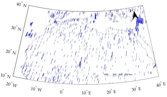
Figure 2.
Hyperion coverage over North Africa.
To reduce the uncertainties associated with the estimated hyperspectral data due to variability in look angle and cloud cover, Hyperion images with view zenith angles less than 5° and total cloud cover less than 10% were selected for the analysis [18]. The view zenith angle threshold was used to minimize BRDF effects. The cloud cover threshold was used to maximize the likelihood of including only cloud-free pixels. Figure 3 shows the number of filtered hyperspectral images for corresponding clusters. Cluster 5 has the largest number of hyperspectral spectra (294), whereas Cluster 4 has the smallest number (74). Nearly all of the clusters have enough image data to derive a representative hyperspectral profile. Among all the clusters, Cluster 13 stands out as an early viable candidate for EPICS based calibration, as it offers lower spatial uncertainty across all the bands and has more contiguous sub regions widely distributed across North Africa. In this paper, the estimation and validation of a representative hyperspectral profile of Cluster 13 are described in detail and Cluster 1 and 4 are briefly presented; the same methodology was used to estimate representative hyperspectral profiles for the remaining clusters.
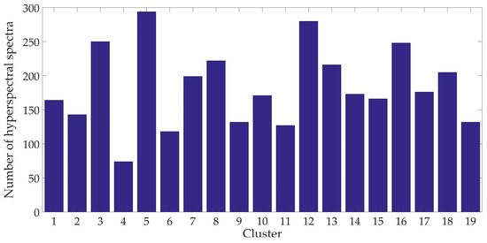
Figure 3.
Number of hyperspectral spectra over different North African clusters.
2.2. Collection of Hyperspectral Data for Cluster 13
Figure 4 shows Cluster 13 spatial extent across North Africa and within this region, Hyperion has imaged 21 different locations. Figure 5 shows the number of hyperspectral spectra corresponding to each World Reference System (WRS)-2 path and row. Among all locations, WRS2 path/rows 177/45, 179/41, and 181/40 were extensively imaged by Hyperion, as they correspond to the well-known Sudan 1, Egypt 1 and Libya 4 PICS, respectively, that have been extensively used for radiometric calibration and stability monitoring of optical satellite sensors. The majority of Cluster 13 locations over North Africa have relatively few images, as Hyperion imaged specified locations upon request. 188 hyperspectral spectra from 16 WRS-2 paths and rows, including all these heavily imaged locations over North Africa and other locations, are used to estimate a representative hyperspectral profile of Cluster 13. 28 spectra from six different locations in North Africa, WRS-2 paths/rows 182/42,198/47, 192/38, 178/43, 185/48, and 200/47, were used to validate the estimated hyperspectral profile of Cluster 13. Validation spectra were chosen from different paths and rows in such a way that they represent the spatial extent of Cluster 13 as shown in solid black rectangle in Figure 4.
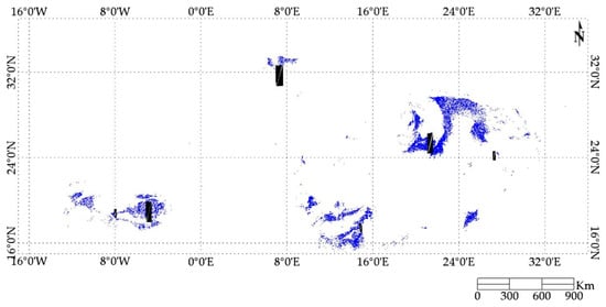
Figure 4.
Extent of cluster 13 over North Africa. Blue color represents cluster 13 pixels. Black rectangle boxed represent the regions used for validation.
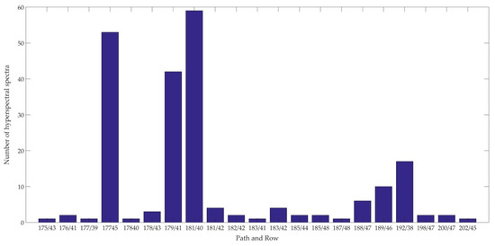
Figure 5.
Number of hyperspectral spectra corresponding to each WRS-2 Paths and Row of Cluster 13.
2.3. Hyperspectral Data for Cluster 13
Two issues were found to have a significant effect on the analysis. The first issue relates to the number of available Hyperion scenes imaging Cluster 13 pixels. 188 Cluster 13 hyperspectral profiles help to derive its reliable representative hyperspectral profile. The second issue relates to the total number of Cluster 13 pixels imaged in a given Hyperion scene; a more representative hyperspectral profile can be generated from a large number of imaged cluster pixels from any WRS-2 path/row. To address the second issue, binary masks identifying cluster 13 pixels within the Hyperion images were generated [19]. Figure 6 shows the Hyperion binary masks for WRS-2 path/rows 181/40, 179/41, 182/42 and 198/47. WRS-2 path/rows 181/40 and 179/41 are among the 15 locations used to derive the hyperspectral profile of Cluster 13 whereas 182/42 and 198/47 are among six locations used for validation of its derived hyperspectral profile. Fortunately, a significant number of Cluster 13 pixels were found in most Hyperion images. Fewer Cluster 13 pixels were found in the image data from WRS-2 path/row 182/42; however, the pixel counts (approximately 15.85% of the total number of image pixels) allowed generation of reliable hyperspectral profiles from those paths and rows, as shown in Figure 6.
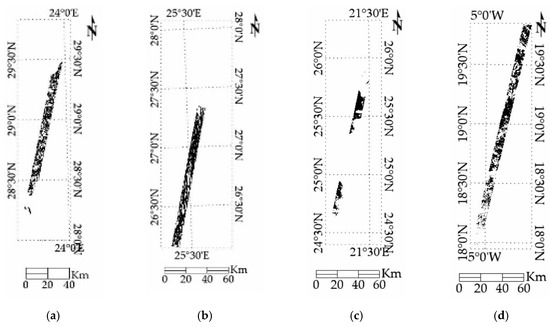
Figure 6.
Cluster 13 Binary Masks: (a) Path/ Row 181/40 (Libya 4), (b) Path/ Row 179/41 (Egypt 1) (c) Path/ Row 182/42 (d) Path/Row 198/47. Black pixels represent Cluster 13 pixels from the Hyperion images.
2.3.1. Data Filtering
Of the 731 hyperspectral images from all the locations of Cluster 13, only 216 images met the required view zenith angle and cloud cover constraints. The Hyperion data were also affected by orbital precession. Beginning in 2011, inclination burns to maintain EO-1’s initial orbital position were stopped due to lack of onboard fuel [9]. As a result, orbital precession effects led to successively earlier local overpass times and increased solar zenith (decreased solar elevation) angles. The larger solar zenith angles resulted in a decreased signal-to-noise ratio due to a longer atmospheric path between the sensor and ground. These effects ultimately led to both absolute and relative changes in the hyperspectral profiles extracted from the image data. Among these two changes, the relative changes are of greater concern, as the SBAF is more affected by any relative change. To determine the absolute and relative changes on the extracted hyperspectral data of Cluster 13, all corrections such as drift correction, application of calibration gains and biases, and BRDF correction were performed first in order to reduce the uncertainty of estimated representative hyperspectral profile of each cluster.
2.3.2. Corrections to Hyperspectral Data
The individual normalized hyperspectral profiles meeting the stability criterion described in the previous section were then corrected to account for potential drift in the sensor response, calibration gain and bias changes, and seasonal variability due to BRDF effects. Each set of corrections is described in further detail below.
Drift correction and Calibration Gain/Bias Application
Generally, satellite sensors exhibit some degree of change in their radiometric response due to mechanical stresses during launch, operation in a harsh space environment, and aging of the sensor itself. Angal et al. [20] and Chander et al. [21] assessed Landsat-7 ETM+ and Terra MODIS radiometric stability using PICS image data. Angal’s analysis found a statistically significant drift in the ETM+ and MODIS Blue band responses. Chander’s analysis confirmed the drifts in the Blue band responses, and also found a statistically significant drift in the ETM+ Red band response.
For this work, it was assumed there is potential drift in the radiometric responses that affect all Hyperion bands. The percentage change in drift was modeled as a linear function of days in a calendar year:
where %/year (reflectance per year) is the percent degradation per year in a band λ, and (reflectance per day) and (reflectance) are the slope and intercept coefficients obtained from a least-squares linear regression of TOA reflectances in band λ. The correction in potential drift for a given band’s hyperspectral profile was then determined as follows:
where is the TOA reflectance of different bands (λ) of Hyperion, Yr is the decimal year representing the acquisition date and overpass time, is the Hyperion TOA profile after yearly drift correction, and is the percent yearly drift of band λ estimated from (1).
For gain and bias correction, the latest set of calibration coefficients reported by Jing et al. [17] should be applied after performing the drift correction:
where and are the calibration gain and bias coefficients for band λ, and is the drift-corrected TOA reflectance.
Four Angle Bidirectional Reflectance Distribution Function (BRDF) Correction
The Bidirectional Reflectance Distribution function defines the interaction of light with a given point on the Earth’s surface by relating incoming and outgoing radiance at that point. BRDF is an inevitable phenomenon for all optical satellite sensors irrespective of their fields of view [22]. Although nominally operated as a nadir-viewing instrument, Hyperion can be pointed to image from different viewing angles. Consequently, BRDF can affect the resulting estimated TOA reflectance, requiring correction [1,2] in order to reduce the uncertainty in the final cross-calibration. Most BRDF models used in cross-calibration research are based on empirical or semi-empirical considerations, as these models tend to be simpler to derive and apply than models based on physical considerations. Angal et al. [20], Liu et al. [23] and Lacherade et al. [2] used Roujean’s BRDF model [24] to remove the angular effect of solar and viewing geometry while performing the cross-calibration of MODIS and MVIRS. Lacherade et al. [2] also used Snyder’s BRDF model to perform cross calibration between different sensor pairs. Wu et al. [25] used the Ross-Li BRDF model to remove the angular effect while determining the calibration stability of MODIS using Libya Desert and Antarctic surface.
Shrestha showed that the BRDF of sand (Algodones dunes) can be modeled as the quadratic function of solar zenith angle [26]. Helder et al. [3] and Mishra et al. [6] derived empirical BRDF models based on linear and quadratic functions of solar zenith angle as part of deriving the absolute calibration model for the Libya 4 PICS, as the solar zenith angle is considered to be the major contributor to BRDF effects. However, the level of correction could be increased if the solar azimuth, view zenith, and view azimuth angles are also considered in the BRDF model. For this work, development of a full four angle model begins with the conversion of the view and solar angles from a spherical coordinate basis to a linear Cartesian basis, in order to obtain the TOA reflectance as a continuous function of independent variables [27]:
where SZA and SAA are the solar zenith and azimuth angles in radians, respectively, and VZA and VAA are the sensor viewing zenith and azimuth angles, respectively (also in radians). Multiple linear least-squares regression is used to derive the following linear model [27]:
Once the model coefficients have been generated, the mean of the solar and sensor view zenith and azimuth angles is chosen as a reference in order to scale the TOA reflectance to a common level. The resulting reference angles are converted to a Cartesian basis, as in Equations (4)–(7), and then used to generate a reference TOA reflectance:
The reference TOA reflectance is then scaled by the ratio of the observed and model predicted TOA reflectances to obtain the final BRDF-corrected TOA reflectance:
Estimation of a Representative Cluster 13 Hyperspectral Profile
After significant yearly drift, calibration gain and bias, and BRDF correction, these hyperspectral data are further analyzed to identify relative changes in the Cluster 13 hyperspectral profiles. 188 individual profiles were optimally normalized with respect to the overall Cluster 13 mean hyperspectral profile.
The optimal normalization constant was found by minimizing the sum of squared residual errors between the mean cluster 13 profile and the individual profiles over a reduced set of wavelengths: A reduced wavelength set consists of the 81 wavelengths from transmission windows in the electromagnetic spectrum which have high transmissivity and have been very widely used for remote sensing purposes, are used to derive optimal constants for all hyperspectral profile.
where is the mean filtered hyperspectral profile of Cluster 13 and is a filtered individual hyperspectral profile.
Once the individual profiles were optimally normalized, absolute differences between the normalized profiles and the mean cluster 13 profile were calculated. Any normalized profile that significantly deviated from the mean profile in any wavelength range was excluded from further analysis because such deviation represents the relative change on the hyperspectral profile which adversely effects the SBAF calculation. With this additional screening step, filtered individual profiles were determined to be suitable for use in generating the representative profile for the cluster.
3. Results
3.1. Pre-processing of Hyperspectral Profiles of Cluster 13
Cluster 13 regions are spread throughout North Africa; as a result, Hyperion had images of Cluster 13 at 21 different location of North Africa. Among these locations, hyperspectral data from 15 locations were used to estimate the hyperspectral profile. These locations were selected for hyperspectral profile estimation for two reasons that increased the reliability of the estimation: (i) the Hyperion images contain a significant number of Cluster 13 pixels, and (ii) Hyperion frequently imaged some of these paths and rows. The hyperspectral data from these 15 locations are subjected to drift correction, application of calibration gain and bias and BRDF correction before using them to estimate the Cluster 13 representative hyperspectral profile.
Drift correction using equations (1) and (2) was applied to 14 Hyperion channels exhibiting statistically significant drift in their response [17]. The resulting hyperspectral profiles are shown in Figure 7, with the red profile representing the original spectrum and the green profile representing the drift-corrected spectrum. The observed drifts were generally small in magnitude (as low as 0.1% per year); the drift-corrected spectrum is virtually indistinguishable from the original spectrum. After application of the drift correction, calibration gains and biases were applied to those channels with significant gain and bias. 25 Hyperion channels have a significant gain (different from unity) and 44 channels have a significant bias (different from 0). Higher wavelength channels have significant gain and bias, so the effect of gain and bias is clearly visible as represented by the blue spectrum in Figure 7. After calibration gain and bias application, the four angle BRDF correction was performed to these spectra. BRDF correction had a greater effect at the wavelength extremes. A minimal correction was observed in effect the 500–600 nm region, as this spectral region transitions between predominant atmospheric scattering and more direct transmission to the surface. BRDF correction was more pronounced at longer wavelengths due to the greater correction of seasonality effects, represented by the cyan spectrum in Figure 7.
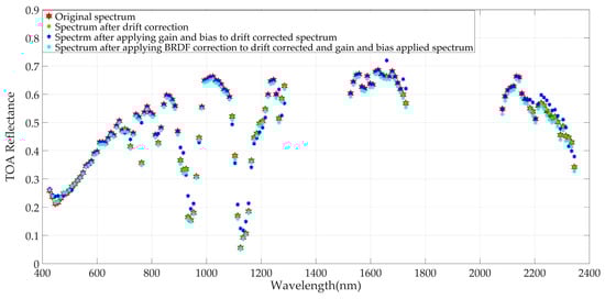
Figure 7.
Corrections applied to the hyperspectral profile. Red symbols represent the original spectrum and cyan symbols represent the corrected hyperspectral data. Highly absorption wavelength ranges are not displayed in the figure.
3.2. Collection of Hyperspectral Profiles of Cluster 13
Figure 8 shows the corrected hyperspectral profiles extracted from different locations of Hyperion image data that are used to estimate a representative Cluster 13 hyperspectral profile. The Hyperion image data are divided into three temporal ranges: (i) from EO-1’s launch to 2007; (ii) 2008 through 2015, and (iii) 2016 to its decommissioning in March 2017. During the first time period, EO-1 flew in the same orbit as Landsat-7 but 1 minute later (green spectra). During the second time period, EO-1 flew in an orbital path approximately 5km below Landsat-7’s path (blue spectra) and began a steady drop in altitude in 2011 that worsened through 2016 to decommissioning (red spectra). The spectrum of the surface is similar from EO-1’s launch to 2015, so the green spectra are overlayed by the blue spectra and aren’t clearly visible in Figure 8.
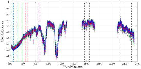
Figure 8.
Hyperspectral data of cluster 13. Green represents the spectra from EO-1’s launch to 2007. Blue represents the spectra from 2008 through 2015 and red represent the spectral from 2016 to its decommissioning in March 2017. Highly absorption wavelength ranges are not displayed in the figure and vertical dashed lines represent typical wavelength ranges of Coastal, Blue, Green, Red, NIR, SWIR 1, and SWIR 2 bands used for remote sensing purposes.
As seen in Figure 8, the post-2016 hyperspectral data are at decreased reflectance levels compared to the pre-2016 data. The decreasing altitude of EO-1’s orbit increased its orbital precession, shifting the local acquisition time progressively earlier and resulting in larger solar zenith angles at the acquisition time; since shadow increases with solar zenith angle, the measured surface reflectance decreases. Assuming the shape of the hyperspectral profile did not significantly change from launch to decommissioning, the decrease in hyperspectral intensity over time will not significantly affect SBAF calculation, since the SBAF is defined as a ratio of reflectances derived from the same profile, in effect, the decrease is “cancelled out” in the SBAF calculation. The primary concern, then, relates to whether the hyperspectral profile shape is exhibiting any significant degree of change over time.
3.3. Investigation of Relative Change of HyperSpectral Profiles of Cluster 13
Figure 9 shows the absolute difference between the individual normalized hyperspectral data and the mean hyperspectral data of cluster 13. Clearly, the absolute difference between the normalized hyperspectral data before 2016 and the mean Cluster 13 data is generally constant within 0.035 reflectance units across all wavelengths, indicating no significant relative change in any hyperspectral profile. The variation in an absolute difference between the normalized individual hyperspectral profiles and mean Cluster 13 hyperspectral profile is due to the spatial variability within Cluster 13, resulting from the threshold used for the initial classification analysis. The absolute differences between three of the pre-2007 and post-2016 hyperspectral data and the mean Cluster 13 data are not constant as represented by green and red dots below 600 nm; having higher absolute difference than −0.04 and green dots which rises rapidly after 2200 nm as shown in Figure 9. These non-constant differences indicate significant relative changes at both shorter and longer wavelengths. These three relatively unstable hyperspectral profiles of Cluster 13 were excluded from further analysis as such relative instability affects the SBAF calculation. Only 185 hyperspectral profiles meet the filter criteria of look angle, cloud cover, and stability in the relative signature. These 185 hyperspectral profiles are thus suitable for estimating the hyperspectral profile of Cluster 13.
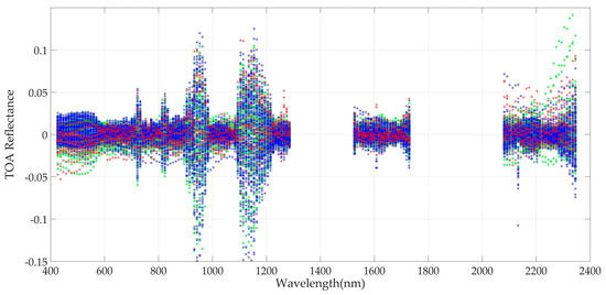
Figure 9.
Absolute difference between the individual normalized hyperspectral data with the mean Cluster 13 hyperspectral data.
3.4. Estimation of a Representative Hyperspectral Profile of Cluster 13
After finding relatively stable hyperspectral measurements of cluster 13, the estimated hyperspectral profile of Cluster 13 is calculated by averaging the 185 hyperspectral data which is shown by the blue curve in Figure 10. The resultant uncertainty is calculated by taking the ratio of the standard deviation to the mean as shown by the red curve in Figure 10. The uncertainty of the VNIR region of Cluster 13 is approximately 5% whereas the SWIR region has less than 4% temporal uncertainty. These observed uncertainties are due to the combination of both temporal and spatial uncertainty of Cluster 13.
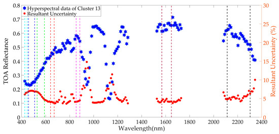
Figure 10.
Estimated representative hyperspectral profile of Cluster 13 and its resultant uncertainty.
3.5. Impact of Atmospheric Parameters on the Hyperspectral Measurements of Cluster 13
Previous studies have shown that the atmosphere contributes to a random uncertainty of about 1% [3,28]. This section discusses the relationship between atmospheric parameters, such as water vapor and aerosol concentration, on the 185 hyperspectral measurements of Cluster 13. These hyperspectral measurements are collected from different locations of North Africa, so it is very challenging to quantify the relationship between the atmospheric parameters and TOA reflectance because the coincident meteorological measurements are rarely available [28,29]. For this analysis, an empirical method is used to study the effect of atmospheric parameters on the TOA reflectance of the Hyperion images.
3.5.1. Water Vapor
Atmospheric water vapor is one of the major contributors to the loss of signal along the atmospheric path. As shown in Figure 8, there are very high absorption features at 950 and 1150 nm due to water vapor. The impact of absorption at these wavelengths is observed by plotting the TOA reflectance of all the spectra of Cluster 13 as shown in Figure 11. TOA reflectance at both of these wavelength ranges from approximately 0.19 to 0.35. A threshold reflectance value is chosen to select the spectra having extreme water vapor quantity. A spectrum having TOA reflectance less than 0.2 is considered to have a high water vapor content, whereas a spectrum having TOA reflectance higher than 0.31 is considered to have a low water vapor content. Based on these thresholds at 950 nm, there are 6 and 15 spectra having high and low water vapor contents, respectively. Similarly, at 1150 nm, there are 3 and 15 spectra having high and low water vapor contents, respectively.
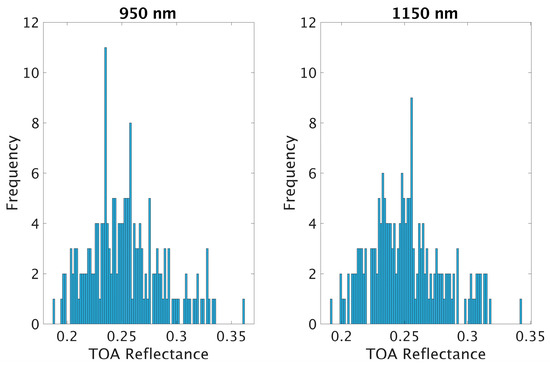
Figure 11.
Range of TOA reflectance at absorptions wavelength, 950 nm (left) and 1150 nm (right).
The mean and standard deviation of these spectra having different water vapor contents are compared with the representative hyperspectral profile of Cluster 13 as shown in Figure 12. The green curve represents the normalized representative hyperspectral profile of Cluster 13. Red and black curves (2 sigma) represent the hyperspectral spectra corresponding to high and low water vapor contents, respectively. There is some expected difference between the hyperspectral spectrum having different water vapor content at the absorption wavelengths. However, in the majority of the spectral regions, error bars of hyperspectral measurement at extreme conditions of water vapor content fall inside the uncertainty range of the representative hyperspectral profile of Cluster 13. This implies that the representative hyperspectral profile can be used for different magnitudes of water vapor quantity.
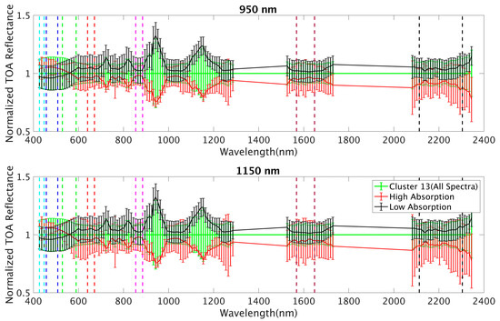
Figure 12.
Comparison of a representative hyperspectral profile of Cluster 13 and hyperspectral measurements having different water vapor content. The green curve represents the normalized hyperspectral profile of Cluster 13. The red curve represents the hyperspectral measurement corresponds to higher water vapor content whereas the black curve represents the hyperspectral measurement corresponding to lower water vapor content. (Error bars = 2 sigma).
3.5.2. Aerosol
In addition to absorption loss, atmospheric aerosol also interferes with the signal received by the optical sensor. Atmospheric aerosol alters the direction and distribution of spectral energy in the beam of light [30]. The impact of atmospheric aerosol is also analyzed using the TOA reflectance at 437 nm as shown in Figure 13. The histogram of TOA reflectance at 437 nm is bimodal, which corresponds to the lower and higher concentration of aerosol. The bimodal histogram has a transition at around 0.23 reflectance, which is used as a threshold for separating the spectra having lower and higher aerosol concentrations. The hyperspectral spectrum with a reflectance value of less than 0.23 at 437 nm is considered to have low aerosol content, whereas the spectrum with reflectance higher than 0.23 is considered to have high aerosol content. Based on the threshold, there are 53 spectra with lower aerosol concentration and 132 spectra with higher aerosol concentration.
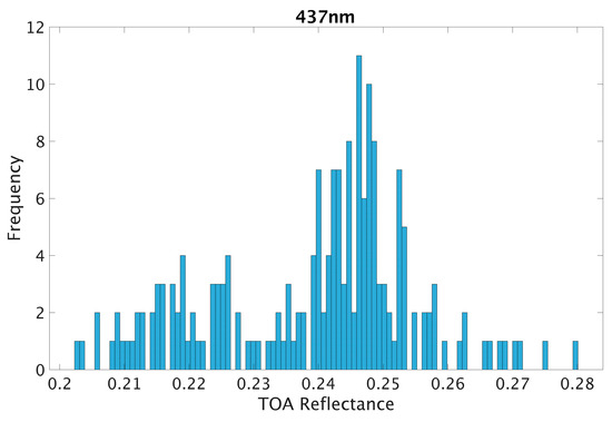
Figure 13.
Histogram of TOA reflectance of the Cluster 13 Hyperion images at 437 nm.
Hyperspectral spectra having a different aerosol concentration is compared with the representative hyperspectral profile of Cluster 13 as shown in Figure 14. The green curve represents the normalized hyperspectral profile of Cluster 13. Red and black curves (2 sigma) represent the mean hyperspectral profile corresponding to lower and higher aerosol concentrations, respectively. From Figure 14, it can be observed that there is more variation in the representative profile of Cluster 13 at a shorter wavelength (<600 nm) than the rest of the spectral regions. This is because the signal at shorter wavelengths is more scattered by the atmospheric aerosol. This results in a reflectance difference of 0.03 between the spectra having the lower and the higher aerosol concentrations. If a reliable aerosol measurement had existed, the effects of aerosol on TOA reflectance could have been quantified. This would help in estimating the separate representative hyperspectral profiles of Cluster 13 with lower uncertainty—one for lower aerosol content and the other for high aerosol content. Since the aerosol measurements are less likely to be available across a continental-scale EPICS, a generic profile with more uncertainty is estimated rather than a separate one for different aerosol concentrations. Furthermore, hyperspectral measurements with different aerosol quantities fall within the uncertainty range of the representative profile of Cluster 13 across all wavelengths. This implies that the representative hyperspectral profile of Cluster 13 can be used for different magnitudes of aerosol quantity.
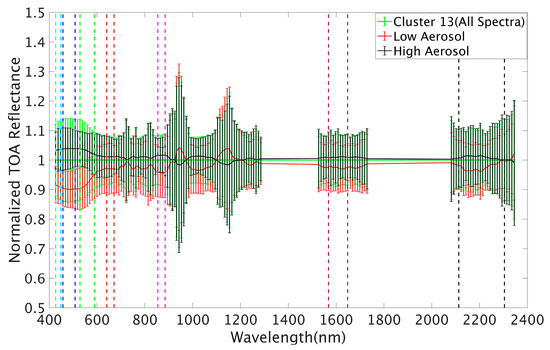
Figure 14.
Comparison of the representative hyperspectral profile of Cluster 13 with the hyperspectral measurements corresponding to low and high aerosol concentration. The green curve represents the normalized hyperspectral profile of Cluster 13. The red curve represents the hyperspectral spectral corresponds to low aerosol concentration higher water vapor content whereas and the black curve represents the hyperspectral spectrum corresponds to higher aerosol concentration (error bars = 2 sigma).
3.6. Estimation of a Representative Hyperspectral Profile for Different Reflectance Clusters
A similar methodology was used to estimate a representative hyperspectral profile of clusters exhibiting different reflectance levels. Among the clusters, Cluster 4 is the darkest cluster and is shown in Figure 15. Overall, Cluster 4 has 43 locations providing 65 spectra suitable for estimation of a representative hyperspectral profile, and another 3 locations providing 6 spectra suitable for validation. The temporal uncertainty over much of the spectral range is approximately 10%, with an additional 1–2% uncertainty at the wavelength extremes.
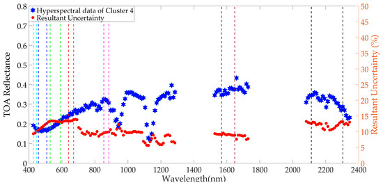
Figure 15.
Estimated representative hyperspectral profile of Cluster 4 and its resultant uncertainty.
The intensity level of Cluster 1 is between those of Cluster 13 and Cluster 4. Cluster 1 has 161 spectra from 56 locations of North Africa which are suitable for estimation and validation of its representative hyperspectral profile. 150 hyperspectral profiles from 53 locations were used to estimate a representative hyperspectral profile of Cluster 1 as shown in Figure 16, and 3 locations provide 6 spectra suitable for validation. The temporal uncertainty for the hyperspectral profile of Cluster 1 is approximately 6 percent for most of the spectral region whereas it exhibits approximately 1% less uncertainty in the shorter wavelengths and 2–3% additional uncertainty at longer wavelengths.
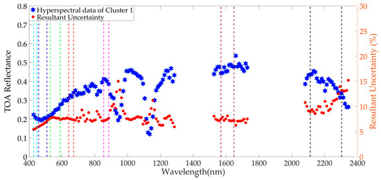
Figure 16.
Estimated representative hyperspectral profile of Cluster 1 and its resultant uncertainty.
Hyperspectral data for the rest of the clusters are estimated with the same procedure and are included in Appendix A.
3.7. Validation of the Estimated Hyperspectral Profile for Cluster 13
3.7.1. Hyperspectral Domain
For validating the hyperspectral spectrum of Cluster 13, spectra from Path/Row 182/42 (mean of 2 spectra), 198/47 (mean of 2 spectra), 192/38 (mean of 17 spectra), 178/43 (mean of 2 spectra), 185/48 (mean of 2 spectra) and 200/47 (mean of 2 spectra) were used. Figure 17 shows the normalized TOA reflectance of the estimated hyperspectral signature of Cluster 13 with its 2-sigma standard deviation and the normalized spectrum from the validation path/rows. The estimated hyperspectral profile of Cluster 13 is used as a reference spectrum for normalizing the hyperspectral profile. As the Cluster 13 hyperspectral profile was used as a reference spectrum for normalization, deviations from unity illustrate the difference between the Cluster 13 spectra and the validation spectra broken down by path/row. These spectra fall inside the uncertainty range of the Cluster 13 spectrum, ensuring that the hyperspectral signatures from those selected paths are the same as the estimated hyperspectral data of Cluster 13. This suggests that the estimated Cluster 13 spectrum can be used to represent the spectrum for any sub region of Cluster 13.
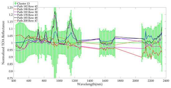
Figure 17.
Validation of hyperspectral spectrum of Cluster 13.
To validate the representative hyperspectral profile of Cluster 4, two spectra each were derived from images of WRS-2 Path/Row 176/40, 202/42 and 198/38. The mean from these three paths/rows were used and all the spectra were normalized to the representative hyperspectral profile of Cluster 4. Figure 18 shows the normalized Cluster 4 profile with a 2-sigma standard deviation (green color), and the normalized spectra from the validation path/rows represented by the blue, red, and black profiles. These spectra lie within the Cluster 4 uncertainty range, suggesting that the estimated hyperspectral profile can be used to represent the spectrum for any of its sub-regions.
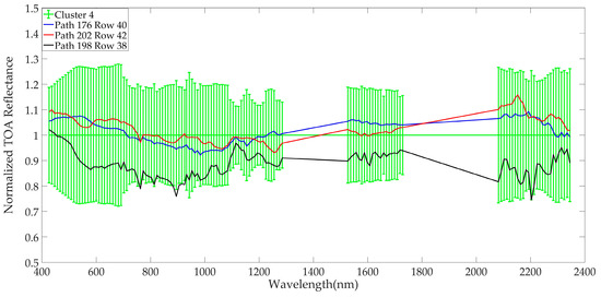
Figure 18.
Validation of hyperspectral spectrum of Cluster 4.
Similarly, hyperspectral validation of the representative hyperspectral profile of Cluster 1 was performed by using two spectra from each of three different WRS-2 Path/Rows: 175/41, 205/44 and 190/47. Figure 19 gives the normalized hyperspectral profile of Cluster 1 (green) and the normalized spectra from the validation path/rows represented by blue, red and black. These spectra lie inside the uncertainty range of a representative hyperspectral profile of Cluster 1 implying that this estimated hyperspectral profile can be used to represent the spectrum for any of its subregions.
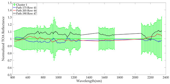
Figure 19.
Validation of hyperspectral spectrum of Cluster 1.
3.7.2. Multispectral Domain
Multispectral validation was performed by comparing the SBAF derived from the hyperspectral data of Cluster 13 and the ratio of multispectral TOA reflectance from two well-calibrated sensors: Landsat 7 ETM+ and Sentinel 2A MSI. The absolute radiometric calibration uncertainty of Landsat 7 ETM+ and Sentinel 2A MSI is 5% and 3%, respectively [31,32,33]. It was assumed that for two well-calibrated sensors, the SBAF is equal to their TOA reflectance ratio. For a multispectral validation, the representative hyperspectral data of Cluster 13 was used and 50 near-coincident (3 days apart) Sentinel 2A MSI/Landsat 7 ETM+ scene pairs were selected from Libya 4 and Egypt 1 since both of these sites were used to estimate the hyperspectral profile of Cluster 13. Among 50 near-coincident scene pairs, 32 were from Libya 4 and the remaining 18 were from Egypt 1. Each sensor’s TOA reflectance was calculated from a region common to Cluster 13 and the corresponding Hyperion images (Figure 6), Sentinel 2A MSI, and Landsat 7 ETM+ images of Libya 4 (Figure 20a,c) and Egypt 1 (Figure 20b,d). The patterns in Figure 16 are due to the dark rock surface in the trough of dunes which are either temporally unstable or classified as a different cluster by unsupervised K-means algorithm.
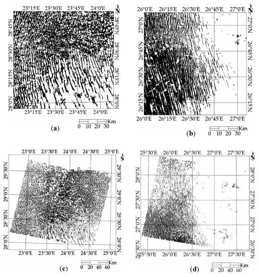
Figure 20.
Cluster 13 binary masks (a) Sentinel 2A MSI Libya 4 (b) Sentinel 2A MSI Egypt 1 (c) Landsat 7 Libya 4 (d) Landsat 7 Egypt 1. Black color pixel represents the Cluster 13 pixels.
The multispectral SBAFs for Libya 4 and Egypt 1 were calculated as the ratio of the Sentinel 2A BRDF-corrected TOA reflectance to the corresponding Landsat 7 TOA reflectances. The BRDF corrections were performed according to the model given in Equations (4)–(10) assuming the Landsat 7 solar and sensor view geometry as the reference.
The hyperspectral SBAF for Cluster 13 was calculated as the ratio of the simulated Sentinel 2A TOA reflectances and the Landsat 7 ETM+ TOA reflectance, as follows:
where: and , respectively, are the simulated TOA reflectance for Sentinel 2A and Landsat 7, is the hyperspectral profile of Cluster 13, and is the relative spectral response of the corresponding sensor.
Figure 21 shows the resulting simulated multispectral SBAFs between Sentinel 2A MSI/Landsat 7 ETM+ and the multispectral TOA reflectance ratios for each band, along with the corresponding 1σ standard deviations. The error bar of the simulated multispectral SBAF is standard deviation of the SBAF calculated using 185 hyperspectral profile of Cluster 13 used to estimate the representative hyperspectral profile of Cluster 13. The error bar of the multispectral SBAF is the standard deviation of the ratio of TOA reflectance of Sentinel 2A and Landsat 7 along with their absolute radiometric uncertainty.
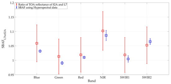
Figure 21.
Plot of simulated multispectral SBAF/Multispectral TOA Reflectance Ratio Comparison (1 sigma).
Overall, the simulated multispectral SBAFs have lower uncertainties due to a large number of hyperspectral data of Cluster 13. The largest difference between the two can be clearly seen in Blue and Green band which is approximately 2.5% and 2.25% whereas the Red band has the smallest different of 0.87% between the simulated multispectral SBAF, derived from hyperspectral profiles of Cluster 13, and the multispectral SBAF. Similarly, the difference between the two sets of SBAF’s is approximately 1.5% for the rest of the bands. As the error bar of multispectral SBAF includes the simulated multispectral SBAF, these two sets of SBAF are statistically indistinguishable for all the bands.
4. Discussion
This work focuses on estimating a representative hyperspectral profile for all clusters. With the assigned hyperspectral profile for clusters, they can be used for both EPICS based cross-calibration of optical satellite sensors [34] and development of EPICS based absolute calibration models. A representative hyperspectral profile for all the clusters was estimated by using the hyperspectral data from the intersection region of Hyperion images and corresponding clusters. The cluster images were filtered for look angles up to ±5° and cloud cover of 10% or less, in order to reduce the uncertainty in the estimated representative hyperspectral profile. In addition to these filters, relative spectral stability of the hyperspectral profiles is also important; any change to the overall shape of the profile yields a different SBAF value, whereas any shift in the intensity level of the spectrum has no effect in SBAF calculation.
It was found that each cluster has a different number of spectra that can be used to estimate the representative hyperspectral profile of each cluster. The majority of the clusters have more than 120 filtered hyperspectral profiles as shown in Figure 3, which provides confidence for the estimated hyperspectral profile of each cluster. In addition, it was found that the largest number of pixels doesn’t guarantee the largest number of hyperspectral profiles; Cluster 3 contains the largest number of pixels (4.3 million pixels) yet has only 250 useable hyperspectral profiles. Among all the clusters, Cluster 5 has the highest number of hyperspectral profiles (294), and Cluster 4 has the lowest number (71) which is still useful for estimating its hyperspectral profile.
The methodology of estimating the hyperspectral profile of North African clusters was demonstrated by using Cluster 13 as it stands out as an early viable candidate for EPICS-based calibration [5]. The resultant uncertainty of the estimated hyperspectral profile of Cluster 13 is approximately 4–5% in the majority of the spectral regions. The resultant uncertainty associated with the representative hyperspectral profile is the combination of both spatial and temporal uncertainties as the representative hyperspectral profile for each cluster is estimated by using hyperspectral spectra collected from different regions of clusters over the EO-1 Hyperion lifetime. It has approximately 5% resultant uncertainty for most of the spectral regions as shown in Figure 10. It has resultant uncertainty of 6% for the wavelengths less than 600 nm which is expected as the spatial uncertainty of Cluster 13 for Coastal/Aerosol and Blue bands are approximately 5%.
Figure 22 presents the comparison of one of the brightest clusters (Cluster 13), the darkest cluster (Cluster 4) and a cluster with an intermediate intensity level. At longer wavelengths, the hyperspectral profiles exhibit more pronounced differences in intensity, providing a wider dynamic range for calibration. Among these three clusters, Cluster 13 has the lowest uncertainty (approximately 5% across all the spectral regions) and Cluster 4 has the highest uncertainty (10% across all the spectral region). The uncertainty is due to the combination of both temporal and spatial uncertainty, more driven by the spatial uncertainty of the clusters. In relative scale, the resultant uncertainty of the Cluster 4 is double to that of the Cluster 13 but in an absolute scale, both of the clusters have similar changes of 0.03 reflectance units across most of the spectral regions as shown in Figure 23.
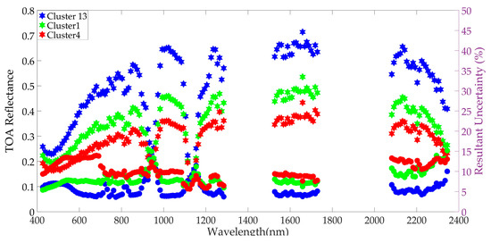
Figure 22.
Comparison of the hyperspectral profile of different clusters with its temporal uncertainty (1-sigma). The solid hexagrams represent a representative hyperspectral profile of a cluster and its corresponding temporal uncertainty is represented by the solid circle of the same color.
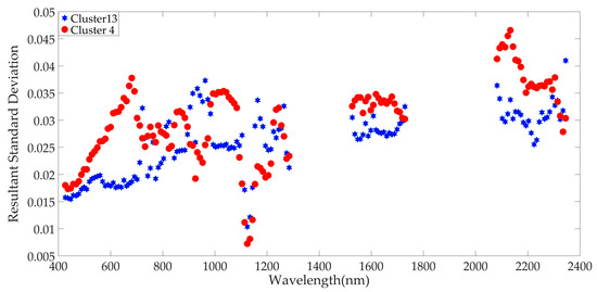
Figure 23.
Comparison of resultant standard deviation (1 sigma) of clusters 13 and 4. The blue and red symbols represent the resultant standard deviation of clusters 13 and 4.
Clusters 13 and 4 have approximately 5% and 12% spatial uncertainty, respectively, across the spectral regions which are expected as the initial analysis of these clusters shows a similar uncertainty level [5]. As the hyperspectral data are only filtered for relative spectral stability, hyperspectral profiles of clusters weren’t filtered for temporal stability which significantly contributed to the resultant uncertainty of the estimated hyperspectral profile. Residual BRDF effects introduce some level of uncertainty into the hyperspectral profile, as the look-angle filtering and the full four-angle correction model do not provide perfect correction. In addition, BRDF correction cannot be performed properly if the cluster doesn’t have a large number of hyperspectral profiles such as Cluster 4. It has the smallest number of hyperspectral profiles (74) due to lower coverage over North Africa, suggesting that it has lower angular sampling than other clusters, which increases the uncertainty of retrieved BRDF parameters [35]. Along with all the above uncertainty, the calibration uncertainty of the EO-1 Hyperion sensor also contributes to the uncertainty of the estimated hyperspectral profiles.
During this analysis, it was observed that most of the hyperspectral profiles of all the clusters are relatively stable over time. Overall, the spectral stability of the representative hyperspectral spectrum of each cluster is similar from 600 nm to 2200 nm as shown in Figure 22 and Appendix A. The representative hyperspectral profile of Clusters 13, 5, 8, 12, 15, and 17 have more resultant uncertainty at spectral range of approximately less than 600 nm than the majority region of the spectrum, i.e., 600–2200 nm. The remaining cluster’s representative hyperspectral profiles have similar resultant uncertainty across the entire wavelength range from 400 nm to 2100 nm. For all the clusters, the resultant uncertainty of the wavelengths higher than 2200 nm has very high resultant uncertainty, almost increasing exponentially as a function of wavelength.
Validation of the representative spectrum data of Cluster 13 was done in both the hyperspectral and multispectral domains. For hyperspectral validation of Cluster 13, six different regions were chosen and hyperspectral spectra from these selected regions were compared with the representative hyperspectral profile of Cluster 13. These hyperspectral profiles from the six regions spectral all lie within the uncertainty of the representative hyperspectral profile of Cluster 13. There is more deviation between the representative and validating spectra of Cluster 13 at the wavelengths less than 600 nm and more than 2000 nm than in the rest of the spectral regions as shown in Figure 17. In contrast, the deviation between the validation and representative spectra of Clusters 1 and 4 is similar across the entire spectral range as shown in Figure 18 and Figure 19.
Similarly, for multispectral validation, 50 near-coincident scene pairs between Sentinel 2A MSI and Landsat 7 ETM+ and the representative hyperspectral profile of Cluster 13 were used. The simulated multispectral SBAF calculated using the representative hyperspectral of Cluster 13 was compared to the multispectral SBAFs (ratio of multispectral TOA reflectance of Sentinel 2A MSI and Landsat 7 ETM+). Blue and Green bands had the largest difference of approximately 2.5% and 2.25% respectively, and the Red band has the smallest difference of approximately 0.87%. These differences are driven by various factors such as spatial uncertainty of Cluster 13, atmospheric uncertainty, BRDF effects and the calibration of the sensors. As the error bar of multispectral SBAF includes the simulated multispectral SBAF, these two sets of SBAF are statistically indistinguishable for all the bands.
Figure 20 shows a common region between Cluster 13 and corresponding Sentinel 2A MSI and Landsat 7 ETM+ images of Libya 4. In the figure, there is a pattern of the dunes which is due to the dark rock in the trough of the dunes formed by the aeolian process; where wind shapes the Earth surface. In large portions of the Libyan desert the wind has scoured the sand to the point it’s reached the hard rock below the surface. So, the deep valleys represent rock not sand and with the sun at solar noon, not shadow. On the windward side of the dunes, heavier particles remain, while on the leeward side the finer particles of sand have been lifted and carried. So for this desert, it’s less about BRDF and shadowing, and much more about how the wind has shaped the dunes, with the dark rock in the valley floors, coarser particles on the windward side which appear to be “medium brightness” and finer particles on the leeward side that appear much brighter. Unsupervised K-means algorithm sees these differences and groups them appropriately. So, these patterns are due to the rock surface which are either unstable over time or classified as a different cluster.
Figure 24 presents the mean resultant uncertainty of the representative hyperspectral profile for each North African cluster. The mean resultant uncertainty was calculated by taking the average resultant uncertainty across all the transmission bands. Since the absorption bands are loosely filtered out, it includes the uncertainty of some of the transition bands across different spectral regions; consequently, the temporal uncertainty is exaggerated and overestimated by approximately 2–3%. For example, Cluster 13 has approximately 5% resultant uncertainty across the majority of its spectral regions, but the mean resultant uncertainty is estimated as approximately 8% in Figure 24.
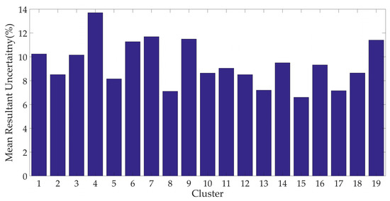
Figure 24.
Comparison of temporal uncertainty of all 19 clusters of North Africa.
Figure 24 shows that a representative hyperspectral profile of Clusters 15 and 4 has the lowest and highest resultant uncertainty, respectively. Cluster 15 is one of the brightest clusters and it spreads wide across North Africa resulting in 166 spectra which helps to estimate a more stable spectrum. Similarly, other clusters such as Clusters 13, 2, 5, and 8 also have comparable uncertainties of approximately 7–8%. The majority of the clusters exhibiting higher uncertainty has lower intensity levels, such as Clusters 1 and 4. As uncertainty is a relative measurement, for the same amount of change in absolute scale, the relative measurement (uncertainty) is higher for the clusters having low intensity than for the clusters having high intensity.
The representative hyperspectral profile for each cluster is estimated using filters such as view zenith angle less than 5° and cloud cover less than 10%. In addition, BRDF correction was further applied to these filtered spectra. So, these representative hyperspectral profiles of different clusters work best for nadir viewing medium and high-resolution optical satellite sensors. As these clusters are estimated using the Hyperion image of all the seasons across the whole of North Africa, a large number of calibration opportunities from all seasons would give a result with lower uncertainty. Whereas, using a fewer number of calibration events would give rise to extra uncertainty, which in turn escalates the overall calibration uncertainty. As the estimated hyperspectral profile is mainly focused on the transmission regions of the electromagnetic spectrum, the profile is not recommended for absorption regions or at spectral regions where there is a sharp gradient in reflectance.
Identification of widespread clusters within North Africa provides a great opportunity to improve PICS-based calibration, as the cluster regions tend to cover much greater areas than the ROIs used in traditional PICS calibration. Overall, the uncertainties of most clusters are within 5% and some are around 10%; but still all are usable for moving from ROI-based PICS calibration to Cluster- based PICS calibration.
Potential extensions to the present work include the following:
- Perform EPICS based cross-calibration and compare it to the cross-calibration gain and bias obtained from an ROI-based cross-calibration approach.
- Generate a cluster-based absolute calibration model and compare its performance to the current absolute calibration model derived for an individual PICS. In contrast to the current approach, the cluster-based approach could potentially offer calibration of any optical satellite sensor on a daily or near-daily basis.
5. Conclusions
A large number of satellite sensors has been launched to monitor changes on the Earth surface. To take advantage of their data, they should be calibrated to a common radiometric scale. Cross-calibration of optical satellite sensors helps to put data from multiple sensors to a common radiometric scale by transferring the calibration from a well-calibrated sensor to an uncalibrated sensor using coincident or near-coincident observations of various targets on the Earth’s surface selected for their temporal stability. Accurate hyperspectral characterization of a target is mandatory for performing cross-calibration as it is used for generating the SBAF required to compensate for differences in relative spectral response (RSR) between sensors.
This work presented a methodology to estimate representative hyperspectral profiles for previously derived clusters of North Africa. Cluster 13 was initially chosen to demonstrate the methodology as it possessed the largest contiguous regions that were widely distributed across North Africa. It also exhibited the lowest overall spatial uncertainty across the VNIR and SWIR spectral range, as well as partial inclusion of the well-known Libya 4 and Egypt 1 PICS within its sub-regions.
The “representative” hyperspectral profile for Cluster 13 in North Africa was estimated for potential use as an extended PICS (EPICS), using 185 hyperspectral profiles derived from 15 WRS-2 Path/Row Hyperion images acquired over its lifetime. The profile exhibited an uncertainty of approximately 5% across all the spectral regions.
Data from WRS-2 Path/Row 182/42, 198/47, 192/38, 178/43, 185/48 and 200/47 were then used to validate the estimated profiles. As the spectra from the selected paths and rows fell within the uncertainty range of the Cluster 13 spectrum, these were used as the “representative” Cluster 13 spectrum. For validation from a multispectral banded perspective, simulated multispectral SBAFs derived from the hyperspectral data were compared to BRDF-corrected multispectral SBAFs (specified as the ratio of TOA reflectance from two well-calibrated sensors). As the error bar of the multispectral SBAFs for MSI and ETM+ includes the simulated multispectral SBAF, these two sets of SBAF are statistically indistinguishable.
Most of the rest of the clusters of North Africa exhibit a resultant uncertainty from 5–12%. Among them, Cluster 15 has the lowest resultant uncertainty of 5% whereas Cluster 4 has the highest uncertainty of around 12%. The major source of uncertainty of the estimated hyperspectral profile is the spatial uncertainty of the cluster itself determined by the threshold used for the initial analysis of the classification of North Africa. In addition, temporal uncertainty of EPICS, residual BRDF effects, and Hyperion calibration uncertainty also contributed some of the resultant uncertainty.
With an accurate hyperspectral signature, any sub-region within Cluster 13 can be used for cross-calibration of optical satellite sensors and also for building an absolute calibration model. Furthermore, hyperspectral profiles for all the clusters found by Shrestha et al., are estimated using a similar methodology, and vast regions of North Africa can be used as EPICS for performing sensor cross-calibration. Using EPICS, the number of coincident and near-coincident scene pairs between sensors to be calibrated is significantly larger than the number obtained using the traditional PICS approach. There is potential that EPICS-based sensor cross-calibration can deliver results of similar or higher quality within a much shorter timeframe than the traditional cross-calibration approach. Furthermore, EPICS-based absolute calibration models will have a significantly larger number of observations which will help to improve the accuracy and consistency of the resulting calibration.
Author Contributions
M.S. conceived the research, developed the algorithm with the help of L.L. and D.H., M.S., L.L., and D.H. analyzed the data, N.H. generated binary mask to filter in the desired pixel of a cluster, M.S. wrote the paper; and L.L. and D.H. edited the paper.
Funding
This research was funded by NASA (grant number NNX15AP36A) and USGS EROS (grant number G14AC00370).
Acknowledgments
The authors would like to thank Tim Ruggles for editing the manuscript and reviewers for their comments that improved the quality of this paper.
Conflicts of Interest
The authors declare no conflict of interest.
Appendix A
In this appendix, we include the estimated representative hyperspectral profile of remaining clusters of North Africa.

Figure A1.
Estimated representative hyperspectral profile of Cluster 2 and its resultant uncertainty.
Figure A1.
Estimated representative hyperspectral profile of Cluster 2 and its resultant uncertainty.


Figure A2.
Estimated representative hyperspectral profile of Cluster 3 and its resultant uncertainty.
Figure A2.
Estimated representative hyperspectral profile of Cluster 3 and its resultant uncertainty.


Figure A3.
Estimated representative hyperspectral profile of Cluster 5 and its resultant uncertainty.
Figure A3.
Estimated representative hyperspectral profile of Cluster 5 and its resultant uncertainty.


Figure A4.
Estimated representative hyperspectral profile of Cluster 6 and its resultant uncertainty.
Figure A4.
Estimated representative hyperspectral profile of Cluster 6 and its resultant uncertainty.


Figure A5.
Estimated representative hyperspectral profile of Cluster 7 and its resultant uncertainty.
Figure A5.
Estimated representative hyperspectral profile of Cluster 7 and its resultant uncertainty.


Figure A6.
Estimated representative hyperspectral profile of Cluster 8 and its resultant uncertainty.
Figure A6.
Estimated representative hyperspectral profile of Cluster 8 and its resultant uncertainty.


Figure A7.
Estimated representative hyperspectral profile of Cluster 9 and its resultant uncertainty.
Figure A7.
Estimated representative hyperspectral profile of Cluster 9 and its resultant uncertainty.


Figure A8.
Estimated representative hyperspectral profile of Cluster 10 and its resultant uncertainty.
Figure A8.
Estimated representative hyperspectral profile of Cluster 10 and its resultant uncertainty.


Figure A9.
Estimated representative hyperspectral profile of Cluster 11 and its resultant uncertainty.
Figure A9.
Estimated representative hyperspectral profile of Cluster 11 and its resultant uncertainty.


Figure A10.
Estimated representative hyperspectral profile of Cluster 12 and its resultant uncertainty.
Figure A10.
Estimated representative hyperspectral profile of Cluster 12 and its resultant uncertainty.


Figure A11.
Estimated representative hyperspectral profile of Cluster 14 and its resultant uncertainty.
Figure A11.
Estimated representative hyperspectral profile of Cluster 14 and its resultant uncertainty.


Figure A12.
Estimated representative hyperspectral profile of Cluster 15 and its resultant uncertainty.
Figure A12.
Estimated representative hyperspectral profile of Cluster 15 and its resultant uncertainty.


Figure A13.
Estimated representative hyperspectral profile of Cluster 16 and its resultant uncertainty.
Figure A13.
Estimated representative hyperspectral profile of Cluster 16 and its resultant uncertainty.


Figure A14.
Estimated representative hyperspectral profile of Cluster 17 and its resultant uncertainty.
Figure A14.
Estimated representative hyperspectral profile of Cluster 17 and its resultant uncertainty.


Figure A15.
Estimated representative hyperspectral profile of Cluster 18 and its resultant uncertainty.
Figure A15.
Estimated representative hyperspectral profile of Cluster 18 and its resultant uncertainty.


Figure A16.
Estimated representative hyperspectral profile of Cluster 19 and its resultant uncertainty.
Figure A16.
Estimated representative hyperspectral profile of Cluster 19 and its resultant uncertainty.

References
- Chander, G.; Mishra, N.; Helder, D.L.; Aaron, D.B.; Angal, A.; Choi, T.; Xiong, X.; Doelling, D.R. Applications of spectral band adjustment factors (SBAF) for cross-calibration. IEEE Trans. Geosci. Remote Sens. 2013, 51, 1267–1281. [Google Scholar] [CrossRef]
- Lacherade, S.; Fougnie, B.; Henry, P.; Gamet, P. Cross calibration over desert sites: Description, methodology, and operational implementation. IEEE Trans. Geosci. Remote Sens. 2013, 51, 1098–1113. [Google Scholar] [CrossRef]
- Helder, D.; Thome, K.J.; Mishra, N.; Chander, G.; Xiong, X.; Angal, A.; Choi, T. Absolute radiometric calibration of Landsat using a pseudo invariant calibration site. IEEE Trans. Geosci. Remote Sens. 2013, 51, 1360–1369. [Google Scholar] [CrossRef]
- Pinto, C.T.; Shrestha, M.; Hasan, N.; Leigh, L.; Helder, D. SBAF for cross-calibration of Landsat-8 OLI and Sentinel-2 MSI over North African PICS. In Proceedings of the Earth Observing Systems XXIII, San Diego, CA, USA, 7 September 2018; p. 107640. [Google Scholar]
- Shrestha, M.; Leigh, L.; Helder, D. Classification of the North Africa Region for Use as an Extended Pseudo Invariant Calibration Sites (EPICS) for Radiometric Calibration and Stability Monitoring of Optical Satellite Sensors. Remote Sens. 2019, 11, 875. [Google Scholar] [CrossRef]
- Mishra, N.; Helder, D.; Angal, A.; Choi, J.; Xiong, X. Absolute calibration of optical satellite sensors using Libya 4 pseudo invariant calibration site. Remote Sens. 2014, 6, 1327–1346. [Google Scholar] [CrossRef]
- Folkman, M.A.; Pearlman, J.; Liao, L.B.; Jarecke, P.J. EO-1/Hyperion hyperspectral imager design, development, characterization, and calibration. In Proceedings of the Hyperspectral Remote Sensing of the Land and Atmosphere, Sendai, Japan, 8 February 2001; pp. 40–52. [Google Scholar]
- Pearlman, J.; Segal, C.; Liao, L.B.; Carman, S.L.; Folkman, M.A.; Browne, W.; Ong, L.; Ungar, S.G. Development and operations of the EO-1 Hyperion imaging spectrometer. In Proceedings of the Earth Observing Systems V, San Diego, CA, USA, 15 November 2000; pp. 243–254. [Google Scholar]
- Franks, S.; Neigh, C.S.; Campbell, P.K.; Sun, G.; Yao, T.; Zhang, Q.; Huemmrich, K.F.; Middleton, E.M.; Ungar, S.G.; Frye, S.W. EO-1 Data Quality and Sensor Stability with Changing Orbital Precession at the End of a 16 Year Mission. Remote Sens. 2017, 9, 412. [Google Scholar] [CrossRef]
- Biggar, S.F.; Thome, K.J.; Wisniewski, W. Vicarious radiometric calibration of EO-1 sensors by reference to high-reflectance ground targets. IEEE Trans. Geosci. Remote Sens. 2003, 41, 1174–1179. [Google Scholar] [CrossRef]
- Green, R.O.; Pavri, B.E.; Chrien, T.G. On-orbit radiometric and spectral calibration characteristics of EO-1 Hyperion derived with an underflight of AVIRIS and in situ measurements at Salar de Arizaro, Argentina. IEEE Trans. Geosci. Remote Sens. 2003, 41, 1194–1203. [Google Scholar] [CrossRef]
- Ungar, S.G.; Pearlman, J.S.; Mendenhall, J.A.; Reuter, D. Overview of the earth observing one (EO-1) mission. IEEE Trans. Geosci. Remote Sens. 2003, 41, 1149–1159. [Google Scholar] [CrossRef]
- Pearlman, J.S.; Barry, P.S.; Segal, C.C.; Shepanski, J.; Beiso, D.; Carman, S.L. Hyperion, a space-based imaging spectrometer. IEEE Trans. Geosci. Remote Sens. 2003, 41, 1160–1173. [Google Scholar] [CrossRef]
- McCorkel, J.; Thome, K.; Ong, L. Vicarious calibration of EO-1 Hyperion. IEEE J. Sel. Top. Appl. Earth Obs. Remote Sens. 2013, 6, 400–407. [Google Scholar] [CrossRef]
- Campbell, P.K.E.; Middleton, E.M.; Thome, K.J.; Kokaly, R.F.; Huemmrich, K.F.; Lagomasino, D.; Novick, K.A.; Brunsell, N.A. EO-1 hyperion reflectance time series at calibration and validation sites: Stability and sensitivity to seasonal dynamics. IEEE J. Sel. Top. Appl. Earth Obs. Remote Sens. 2013, 6, 276–290. [Google Scholar] [CrossRef]
- Czapla-Myers, J.; Ong, L.; Thome, K.; McCorkel, J. Validation of EO-1 Hyperion and Advanced Land Imager Using the Radiometric Calibration Test Site at Railroad Valley, Nevada. IEEE J. Sel. Top. Appl. Earth Obs. Remote Sens. 2016, 9, 816–826. [Google Scholar] [CrossRef]
- Jing, X.; Leigh, L.; Helder, D.; Pinto, C.T.; Aaron, D. Lifetime Absolute Calibration of the EO-1 Hyperion Sensor and Its Validation. IEEE Trans. Geosci. Remote Sens. 2019, 1–10. [Google Scholar] [CrossRef]
- EROS, U. USGS EROS Archive - Earth Observing One (EO-1). Available online: https://www.usgs.gov/centers/eros/science/usgs-eros-archive-earth-observing-one-eo-1?qt-science_center_objects=0#qt-science_center_objects (accessed on 4 September 2017).
- Hasan, M.N.; Shrestha, M.; Leigh, L.; Helder, D. Evaluation of an Extended PICS (EPICS) for Calibration and Stability Monitoring of Optical Satellite Sensors. Remote Sens. 2019, 11, 1755. [Google Scholar] [CrossRef]
- Angal, A.; Choi, T.; Chander, G.; Xiong, X. Monitoring on-orbit stability of Terra MODIS and Landsat 7 ETM+ reflective solar bands using Railroad Valley Playa, Nevada (RVPN) test site. In Proceedings of the Geoscience and Remote Sensing Symposium, Boston, MA, USA, 7–11 July 2008; pp. IV-1364–IV-1367. [Google Scholar]
- Chander, G.; Xiong, X.J.; Choi, T.J.; Angal, A. Monitoring on-orbit calibration stability of the Terra MODIS and Landsat 7 ETM+ sensors using pseudo-invariant test sites. Remote Sens. Environ. 2010, 114, 925–939. [Google Scholar] [CrossRef]
- Roy, D.P.; Zhang, H.; Ju, J.; Gomez-Dans, J.L.; Lewis, P.E.; Schaaf, C.; Sun, Q.; Li, J.; Huang, H.; Kovalskyy, V. A general method to normalize Landsat reflectance data to nadir BRDF adjusted reflectance. Remote Sens. Environ. 2016, 176, 255–271. [Google Scholar] [CrossRef]
- Liu, J.-J.; Li, Z.; Qiao, Y.-L.; Liu, Y.-J.; Zhang, Y.-X. A new method for cross-calibration of two satellite sensors. Int. J. Remote Sens. 2004, 25, 5267–5281. [Google Scholar] [CrossRef]
- Roujean, J.L.; Leroy, M.; Deschamps, P.Y. A bidirectional reflectance model of the Earth’s surface for the correction of remote sensing data. J. Geophys. Res. Atmos. 1992, 97, 20455–20468. [Google Scholar] [CrossRef]
- Wu, A.; Xiong, X.; Cao, C.; Angal, A. Monitoring MODIS calibration stability of visible and near-IR bands from observed top-of-atmosphere BRDF-normalized reflectances over Libyan Desert and Antarctic surfaces. In Proceedings of the Earth Observing Systems XIII, San Diego, CA, USA, 21 August 2008; p. 708113. [Google Scholar]
- Shrestha, M. Bidirectional Reflectance Distribution Function of Algodones Dunes. Master’s Thesis, South Dakota State University, Brookings, SD, USA, 2016. [Google Scholar]
- Farhad, M.M. Cross Calibration and Validation of Landsat 8 OLI and Sentinel 2A MSI. Master’s Thesis, South Dakota State University, Brookings, SD, USA, 2018. [Google Scholar]
- Chaulagain, Y. An Analysis on the Correlation Between Atmospheric Parameters and TOA Reflectance of Pseudo Invariant Calibration Sites (PICS). Master’s Thesis, South Dakota State University, Brookings, SD, USA, 2019. [Google Scholar]
- Schowengerdt, R.A. Remote Sensing: Models and Methods for Image Processing; Elsevier: Amsterdam, The Netherlands, 2006. [Google Scholar]
- Schott, J.R. Remote sensing: The Image Chain Approach; Oxford University Press on Demand: Oxford, UK, 2007. [Google Scholar]
- Markham, B.L.; Thome, K.J.; Barsi, J.A.; Kaita, E.; Helder, D.L.; Barker, J.L.; Scaramuzza, P.L. Landsat-7 ETM+ on-orbit reflective-band radiometric stability and absolute calibration. Trans. Geosci. Remote Sens. 2004, 42, 2810–2820. [Google Scholar] [CrossRef]
- Markham, B.L.; Haque, M.O.; Barsi, J.A.; Micijevic, E.; Helder, D.L.; Thome, K.J.; Aaron, D.; Czapla-Myers, J.S. Landsat-7 ETM+: 12 years on-orbit reflective-band radiometric performance. IEEE Trans. Geosci. Remote Sens. 2012, 50, 2056–2062. [Google Scholar] [CrossRef]
- Gascon, F.; Bouzinac, C.; Thépaut, O.; Jung, M.; Francesconi, B.; Louis, J.; Lonjou, V.; Lafrance, B.; Massera, S.; Gaudel-Vacaresse, A. Copernicus Sentinel-2A calibration and products validation status. Remote Sens. 2017, 9, 584. [Google Scholar] [CrossRef]
- Shrestha, M.; Hasan, M.; Leigh, L.; Helder, D. Extended Pseudo Invariant Calibration Sites (EPICS) for the Cross-Calibration of Optical Satellite Sensors. Remote Sens. 2019, 11, 1676. [Google Scholar] [CrossRef]
- Franch, B.; Vermote, E.; Skakun, S.; Roger, J.-C.; Masek, J.; Ju, J.; Villaescusa-Nadal, J.L.; Santamaria-Artigas, A. A Method for Landsat and Sentinel 2 (HLS) BRDF Normalization. Remote Sens. 2019, 11, 632. [Google Scholar] [CrossRef]


© 2019 by the authors. Licensee MDPI, Basel, Switzerland. This article is an open access article distributed under the terms and conditions of the Creative Commons Attribution (CC BY) license (http://creativecommons.org/licenses/by/4.0/).