Potential of Smartphone SfM Photogrammetry to Measure Coastal Morphodynamics

Abstract

With recent advances in photogrammetric processing methods and sensor technologies, smartphones represent a new opportunity of mainstream, low-cost sensor, with a great potential for Structure-from-Motion (SfM) photogrammetry, and in particular for participatory science programs or citizen observatories. Keeping in mind the application in citizen observatories, three smartphone models (Galaxy S7®, Lumia 930® and iPhone 8®) and a bridge camera were compared (separately and in combination) for coastal applications: A coastal cliff and a sandy beach. Various acquisition protocols, at different distances from a cliff face and using “linear” or “fan-shaped” capture mode, were also assessed in their efficiency. A simultaneous Terrestrial Laser Scanner (TLS) survey provided a reference dataset to assess the quality of the SfM reconstructions. Satisfactory reconstructions (mean error < 5 cm) of the cliff face were obtained using all smartphone models tested. To measure the cliff face, fan-shaped capturing mode allowed a quicker image acquisition on site and better results (mean error of 1.3 cm with a standard deviation of 0.1 cm at 20 m from the cliff face) than linear capturing mode (mean error of 2.5 cm with a standard deviation of 21.8 cm), provided that the distance to the cliff face is sufficient to ensure a good image overlap. To obtain satisfactory results over beaches, we show that it is preferable to have high-angle shots of the study area, which may limit the applicability of the method for certain sites.

1. Introduction

Situated at the interface between marine and terrestrial environments, coastal zones are exposed to a combination of several morphological processes, as well as anthropogenic pressure. A better understanding of the mechanisms driving shoreline change is essential for improved coastal risks management. This involves suitable monitoring strategies, implying recurrent surveys, adapted to the environmental constraints (meteorological conditions, limited survey duration, etc.), and to the different types of coastal environments, and covering a range of spatial (from decimetre to kilometre) and temporal scales (from event to seasonal). Depending on the study area, a multi-source monitoring may be carried out, including different techniques, from wide-covering methods such as satellite imagery to point-wise measurements with GPS surveys [1].

Differential Global Positioning System in Real Time Kinematic (RTK DGPS) mode or tachometer are the most common techniques for beach surveying [2]. These point-wise methods are associated with high accuracy, but low spatial resolution. Easy-to-use, they can be suitable for recurrent long-term surveys [3,4], generally through the acquisition of cross-shore profiles. However, they can be very time-consuming and involve a great human effort for large areas. Besides, they are not suitable to survey cliff fronts.

During the last decades, various high-resolution remote sensing techniques have proved their potential for coastal monitoring, allowing data spatialization. Coastal video monitoring provides high-frequency, continuous and autonomous observations [5,6,7,8]. Yet, such systems require an infrastructure (pole or building for implementation, power supply, etc.) and the feasibility is therefore very dependent on the study site configuration and anthropization. Furthermore, the wide-angle field of view results in large spatial heterogeneity in data quality [6].

Terrestrial Laser Scanner (TLS) is an optical active remote sensing technology. Most TLSs use the time-of-flight of the laser pulses reflected by the environment to measure point positions. Providing dense point clouds with centimetric accuracy, TLS are commonly used for coastal monitoring [9,10,11].

Owing to technological progress and decreasing cost of Unmanned Aerial Vehicles (UAVs), as well as recent development of the Structure-from-Motion (SfM) approach in photogrammetry, the potential of UAV photogrammetry for coastal surveys has been demonstrated for several years [12,13,14,15]. UAVs enable the rapid acquisition of high-resolution (<5 cm) topographic data at low cost.

By providing different points of view (terrestrial or aerial), TLS and UAV can be used in combination [16,17,18]. Nevertheless, these methods require favorable weather conditions (low wind, no rain) and experienced operators, which may prevent measurements during periods, such as spring tides or post-storm events, during which important morphological changes can occur.

To avoid these drawbacks, terrestrial photogrammetry [17,19] appears as a very flexible monitoring technique given adequate view point of the study area. By making in situ surveys easier, this approach is more likely to be used on different study sites by different operators in parallel.

With miniature cameras inside smartphones becoming more and more efficient, smartphones also appear as a new opportunity of a mainstream, low-cost sensor, which can be particularly useful for participatory science programs or citizen observatories. Smartphone photographs have already been used in sciences for coastal applications, such as the CoastSnap beach monitoring initiative, which gathers crowd-sourced photographs at some iconic beaches for shoreline detection [20]. Al-Hamad and El-Sheimy [21] tested smartphones as mobile mapping systems, using exterior orientation parameters computed by photogrammetry to improve position and orientation measurements. However, we note that few studies make use of smartphones for stereo-photogrammetric applications. Kim et al. [22] tested the feasibility of using a single smartphone as the payload of a photogrammetric UAV-system. This use appears problematical in dynamic mode. Micheletti et al. [23] successfully performed SfM-photogrammetry restitution of river banks from terrestrial smartphone surveys. They achieved centimeter-precision terrain reconstructions at close-range (10 m or less). Prosdocimi et al. [24] obtained a Digital Elevation Model (DEM) from an 8 mega-pixel iPhone5® camera, with a resolution of 0.1 m and a Root Mean Square (RMS) error of 5.7 cm. They suggested that this approach can be an alternative low-cost methodology to analyze bank erosion in agricultural drainage networks. Ozturk et al. [25] used smartphone SfM-photogrammetry for structural geology applications, extracting Ground Control Points (GCP) from previously existing data and achieving decimetric accuracy.

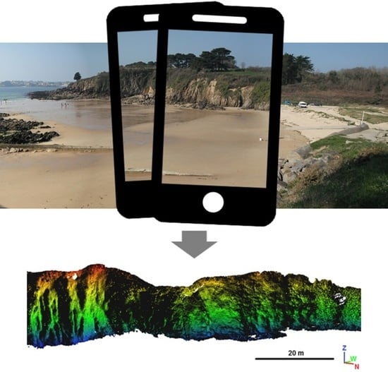
This study proposes to use terrestrial SfM photogrammetry from smartphone photographs for coastal monitoring. From a geometric point of view, it appears easier to reconstruct vertical objects compared to horizontal objects using terrestrial close-range SfM photogrammetry. Firstly, we test the method to survey a portion of a coastal cliff face. Secondly, we assess the potential of the method to reconstruct beach morphology. During the tests, we evaluated three smartphone models and different acquisition protocols in terms of their efficiency.

2. Study Area

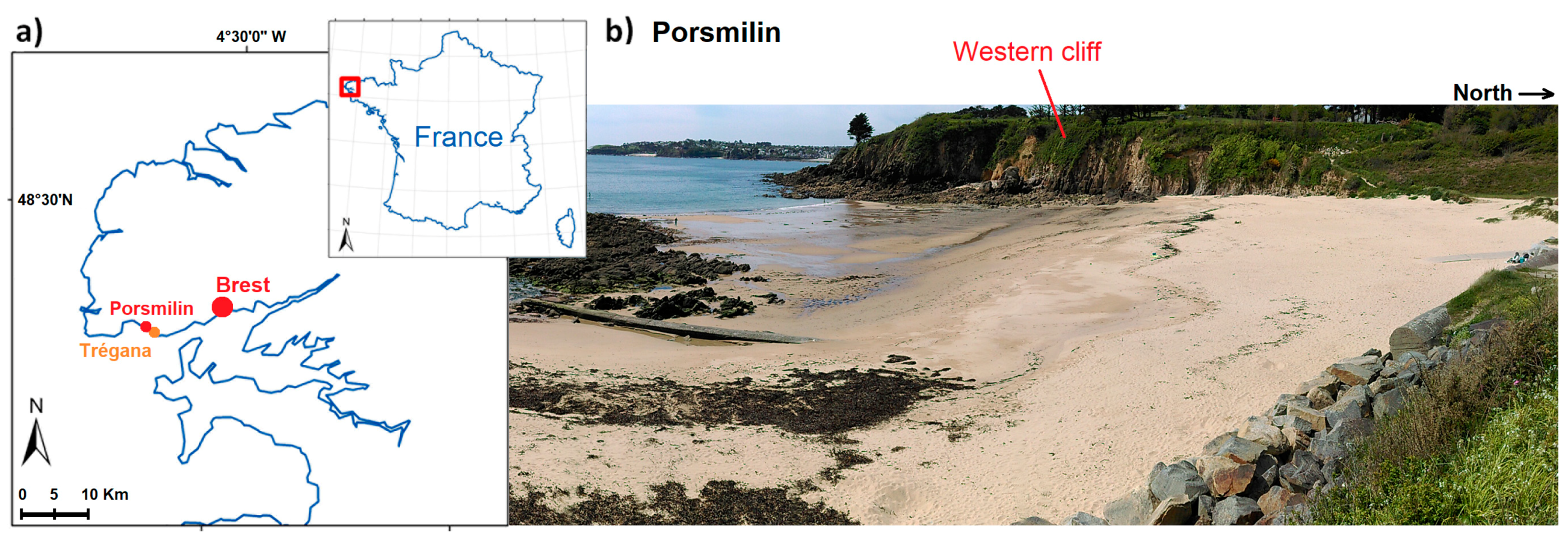
The study site is Porsmilin Beach, located at the entrance of the Bay of Brest in Brittany, France (Figure 1). The beach is slightly-anthropized, the only infrastructures being a car park (at the north-east, around 3 m above the beach), a jetty and a concrete pipe on the east. The beach stretches over 170 m alongshore and, at low-tide, it uncovers for over 200 m cross-shore. Eastward and westward, it is surrounded by orthogneiss cliffs of about 15 m in height. The beach is backed to the north by a brackish-water marsh that no longer communicates with the sea. The back-beach dune is between 1 m high to 1.8 m high. The average beach slope extracted from cross-shore profiles is around 3°, with higher profile variability between 25 m and 70 m. The environment is macrotidal, with a mean spring tidal range of 5.7 m, and subject to mean annual wave height around 1 m and storm waves over 2 m.

This site has been chosen for the tests because it is monitored in the framework of the national DYNALIT (Littoral and Coastline Dynamics) observatory [14]. In this context, a TLS survey was carried out simultaneously to the smartphone SfM photogrammetry survey. The 3D data resulting from this TLS survey, encompassing the beach and the cliff, are used as validation data.

3. Materials and Methods

3.1. Cameras

Compared to reflex or bridge cameras, smartphones are equipped with smaller-diameter lenses and smaller sensors with smaller photosites, which gather less light and offer a lower ISO range. In theory, this would be prejudicial to image quality, but smartphones compensate the small sensors by improved computational power. Furthermore, the focal length of smartphone cameras is very short, which generally is not recommended for photogrammetric applications, as in this case lens distortion modeling is more challenging. Nevertheless, smartphone cameras are fixed lenses and have now a reasonably high resolution (>5 Mpix), which are favored for SfM photogrammetry.

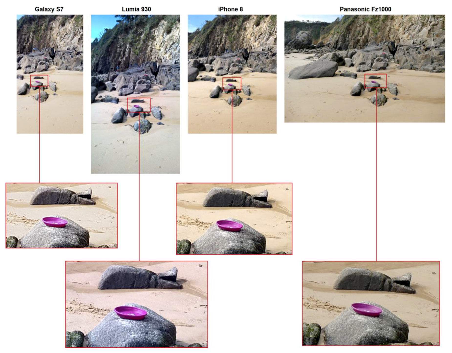
Three models of smartphones were tested to assess if the quality of the topographic reconstruction varies from one model to another or, in a participatory science prospect, if it is possible to combine photographs taken by different smartphones in the reconstruction process. The models used in this study are the Samsung® Galaxy S7, the Nokia® Lumia 930 and the Apple® iPhone 8. Their main properties (given by manufacturers) are summarized in

Table 1. Characteristics of various models of smartphone cameras and of a bridge camera.

	Galaxy S7	Lumia 930	iPhone 8	Panasonic Lumix FZ1000 (Bridge Camera)
Focal length (mm)	4.2	4.46	3.99	9.12
35 mm equivalent focal length (mm)	26	28	28	25
Image size (pixels)	4032 × 2268 (10 Mpix)	5376 × 3024 (20 Mpix)	4032 × 3024 (12 Mpix)	5472 × 3648 (20 Mpix)
Pixel size on the sensor (µm)	1.38675 × 1.38675	1.11731 × 1.11731	1.22331 × 1.22331	2.4 × 2.4
Color depth	24	24	24	24
ISO sensitivity	ISO-40	ISO-64	ISO-20	ISO-125
Use in this study	Test 1 (Porsmilin cliff) Test 2 (Porsmilin cliff) Test 3 (Porsmilin beach)	Test 1 (Porsmilin cliff) Trégana Beach	Test 1 (Porsmilin cliff)	Test 1 (Porsmilin cliff)

. In parallel, a Panasonic® FZ1000, a top-end bridge camera (Table 1) is also tested to compare smartphone reconstructions to the results obtained with a more “classical” camera for terrestrial photogrammetry. An example of photographs collected by the different cameras is presented in Figure 2.

3.2. SfM Photogrammetry Processing

In the last decades, the development of Structure-from-Motion (SfM) photogrammetry has contributed to make the acquisition procedure considerably easier. Indeed, SfM photogrammetry induces: (i) more flexibility in photographs collection, (ii) more flexibility in the choice of the cameras, (iii) camera pre-calibration is no longer necessary, and (iv) photos collected from various cameras can be mixed in the same dataset.

The datasets are processed using Agisoft® PhotoScan Pro (v. 1.2.6), a commercial SfM and image matching software. The algorithm for surface reconstruction is divided into three main steps:

• Image orientation by bundle adjustment (detection and matching of homologous keypoints on overlapping photographs in order to compute the external parameters for each camera).
• Refinement of camera calibration parameters (internal parameters) including Ground Control Points (GCPs) positions. GCPs, consisting of highly visible targets, are manually pointed on the images, their ground positions being measured by RTK DGPS. These GCPs are used to improve camera auto-calibration and to georeference the dataset. In PhotoScan, the lens distortion is modelled using Brown’s distortion model.
• Dense image matching to produce a dense point cloud using the estimated external and internal camera parameters.

For this study, the same operator processed all the datasets. The photographs were not pre-selected but some of them were automatically discarded during the processing. As far as possible, the same parameters were kept from one processing to another. Masks were applied on the sky and on the sea to avoid false tie point detection on these areas. The dense point cloud can be rasterized on a regular grid to produce a DEM and an orthophotograph. However, for sub-vertical objects, here the cliff measurements, the raw dense point cloud was used.

3.3. Positioning and Validation Data

3.3.1. RTK DGPS Measurements

Taking advantage of an existing geodetic marker on the study site to set up our GPS base station, RTK DGPS is simple to implement, achieving centimetric positioning accuracy. The device used for this study is a Topcon® HiPer V GNSS receiver.

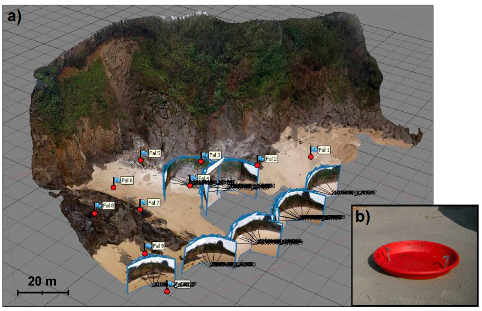
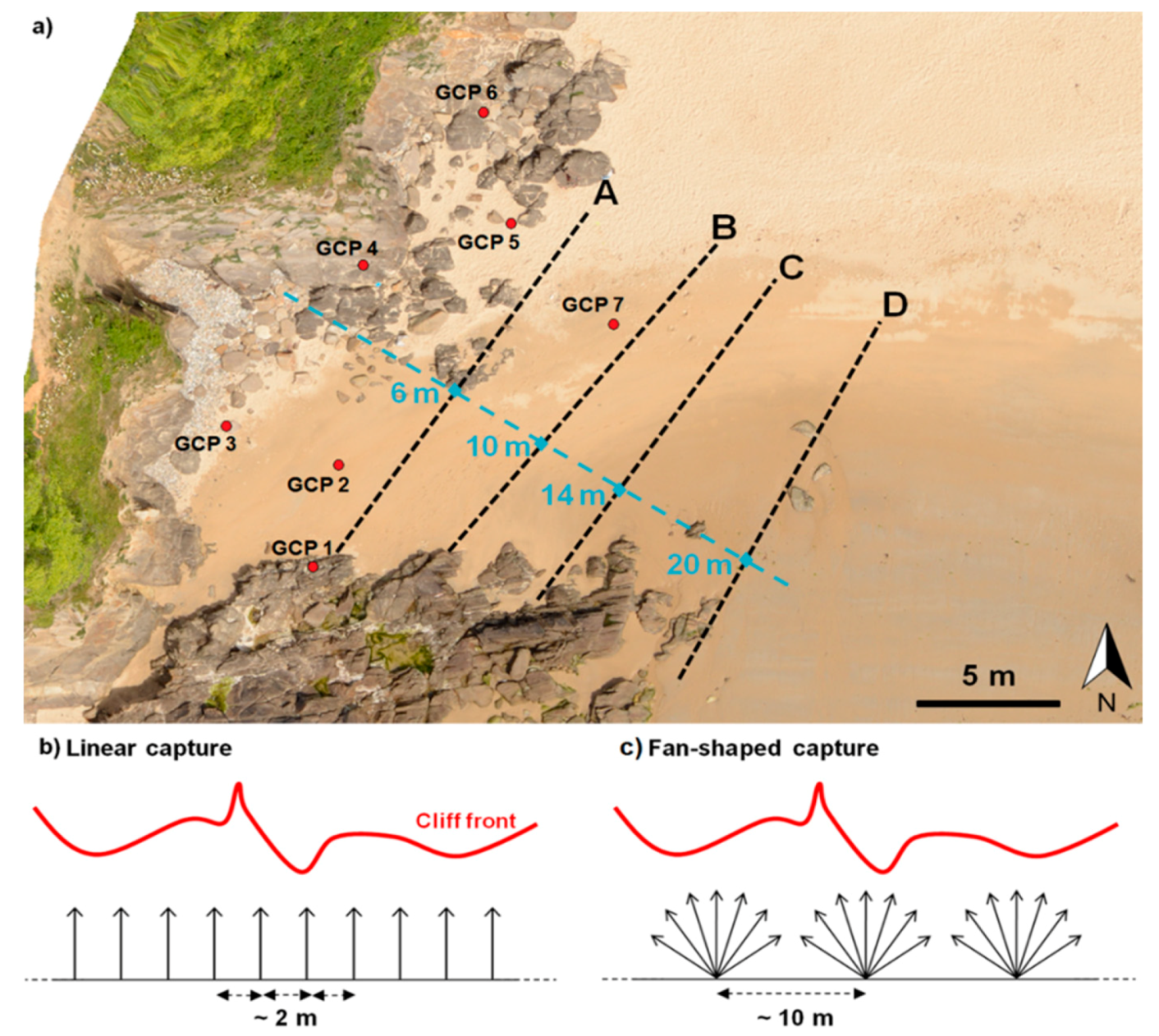
For the TLS survey, RTK DGPS was used to measure the position of reflective targets distributed around the TLS standpoint before the survey. These targets are cylinders 10 cm in diameter and 10 cm in height. For the SfM-photogrammetric survey, we used the RTK DGPS to measure the position of the GCPs, which in this case are red or purple circular targets 30 cm in diameter.

3.3.2. TLS Data

As mentioned previously, Porsmilin beach is part of the DYNALIT long-term coastal observatory and is therefore regularly monitored. In this context, a TLS survey was performed simultaneously to the smartphone photogrammetric test. The TLS device was a Riegl® VZ-400. In the present study, the TLS survey involved two scans from two distinct scan positions, each covering 360° horizontally and 100° (from 30° to 130°) vertically with an angular resolution of 0.04° in both directions. With a range of up to 600 m, each point cloud has more than 20 million points.

Data processing was then performed using the RiScanPRO® software suite (provided by Riegl®). It comprised two main steps:

(i)

Georeferencing and individual clouds assembly. An indirect georeferencing was performed [9], using 21 reflective targets.

(ii)

Manual point cloud filtering to remove artifacts or undesirable data (people on the beach, data outside of the study area, etc.)

Finally, meshes are generated separately on the beach and on the studied cliff face using CloudCompare®, a 3D point cloud freeware processing software. We used a 2.5D Delaunay triangulated mesh for the beach and a Poisson 3D surface reconstruction for the cliff [26].

This dataset is used as validation data to assess accuracy of the SfM photogrammetric point clouds. This assessment is performed using the “cloud-to-mesh distance” tool, computing nearest-neighbor distances in CloudCompare. Using a mesh for the TLS dataset avoids computational artifacts in quality assessment due to a heterogeneous point cloud density.

4. Survey Operational Mode

4.1. Description of the Cliff Face Surveys

Different tests were carried out to survey a 25 m long portion of the western cliff face (Figure 1 and Figure 3). The first test compares the three different smartphone cameras (Galaxy S7, Lumia 930 and iPhone 8) and the Panasonic® FZ1000 bridge camera. Photographs were collected from different viewpoints ranging from 5 to 20 m from the cliff face (Figure 3). Smartphone photographs were collected with a portrait orientation, as this is more intuitive when using smartphone screens. During the survey, the operator took care of keeping a sufficient overlap (around 60 to 80%) between photographs. As the photographs have different sizes depending on the device (Figure 2), the number of collected photographs varies from one dataset to another: 58 photographs for the Galaxy S7, 55 for the Lumia 930, 38 for the iPhone 8 and 25 for the bridge camera Panasonic Fz1000. The lower number of photographs with the bridge camera is also due to the landscape layout, which allowed for maximizing image overlap.

The image datasets from the different devices were initially processed separately before processing all photographs from the various smartphones as a single dataset. As already mentioned, using a 2.5D DEM is irrelevant for the measurement of the cliff face. Thus, a dense point cloud was used in this case. All datasets were georeferenced in RGF93-Lambert93 (EPSG: 2154), which is the official coordinate system in France. For this test, 10 GCPs (identified by a flag in Figure 3), were distributed throughout the study area.

A second test was performed using the Galaxy S7 to compare different survey protocols, and more particularly the impact of (i) the distance to the cliff face and (ii) the geometry of the image network (which we call shot mode). For this test, photographs were collected from four segments (named A, B, C and D on Figure 4), around 20 m long, nearly parallel to the cliff and located respectively at 6 m, 10 m, 14 m and 20 m from the cliff foot (Figure 4a). For each segment, photographs were collected according to two shot modes, respectively “linear capture” and “fan-shaped capture”. In linear capture mode, one photograph was taken every 2 m along a segment (Figure 4b). In fan-shaped capture mode, seven divergent photographs were taken from three different viewpoints for each segment, covering an angle of about 160° (Figure 4c). So, for the same survey duration, more photographs were collected with fan-shaped capture mode than with linear capture mode. For this second comparison test, seven GCPs were used (Figure 4a).

According to the Agisoft PhotoScan User Manual, a linear capture mode is more appropriate than a fan-shaped capture (for façade reconstruction), to limit divergence between photographs. However, by multiplying the positions of fan-shape capture (here three different positions), photographs taken from these different viewpoints converge, which should provide a satisfactory image acquisition geometry.

4.2. Description of the Beach Survey

Regardless of the camera used, reconstructing almost horizontal beach topography by terrestrial photogrammetry is challenging because of the nearly tangential line of sight. It is advisable to capture photographs using as high-angle shots as possible, using overlooking points of view if possible, without putting the operator at risk. Such a method is therefore not practicable at every beach site.

Several positions for photography acquisition were tested for Porsmilin: Including from the top of the western cliff, from the back-beach small dunes, and from the north-east car park. The only set of positions that appears to be compatible with a SfM processing, is the one situated atop the western cliff, as depicted by stars on Figure 5. Using five viewpoints, 34 photographs were collected using the Galaxy S7 smartphone with a fan-shaped capture (linear capture was impossible because of vegetation creating occlusions or precluding access). On the distant parts of the study area, the ground sampling distance and pixel deformation increased due to oblique camera angles, and hence some of the targets distributed on the beach to be used as GCPs were harder to identify. Eight GCPs (out of the 23 installed) could not be detected or were visible on a single photograph, and as a result were not used during processing (Figure 5).

5. Results

5.1. Test 1: Comparison of Smartphone Models to Reconstruct the Cliff Face

This first test compares the reconstructions of the cliff face from photograph datasets (example in Figure 3) collected separately by three different smartphones, a dataset collected with a top-end bridge camera and a dataset mixing all Smartphones’ photographs. As mentioned in Section 4.1, the number of images collected depends of the width of the photograph. From one dataset to another, the rate of aligned photographs after processing varies slightly (with the number of unaligned images ranging from 0 to 14,

Table 2. Mean density and standard deviation obtained on the dense point clouds reconstructed from the different datasets.

	Used/Collected Number of Photographs	Dense Point Cloud Mean Density	Standard Deviation in the Density of the Dense Point Cloud
Galaxy S7 (G7)	46/58	1968 pts/m2	750 pts/m2
Lumia 930 (L930)	41/55	2667 pts/m2	923 pts/m2
iPhone 8 (i8)	38/38	1940 pts/m2	749 pts/m2
G7 + L930 + i8	125/154	2305 pts/m2	575 pts/m2
Panasonic FZ1000	25/25	3172 pts/m2	1190 pts/m2

). The dataset with most discarded images corresponded to the Galaxy S7 and the Lumia 930, whose photographs are less wide. The line of sights of the external photographs are probably too tangential to the cliff face for tie points to be correctly identified.

The mean density of the resulting dense point clouds varies from 1940 points/m² with the iPhone 8 dataset to 2667 points/m² with the Lumia 930 (Table 2). These variations can be due to the different camera characteristics, particularly the number of pixels and the physical pixel size on the sensor. The density of the point cloud is not denser for the mixed dataset, but the standard deviation representing spatial variability (575 points/m²) is lower. The Panasonic FZ1000 bridge camera leads to a denser point cloud, with 3172 points/m² (Table 2). The high standard deviation in the density of the point clouds can be due to the non-linear geometry of the cliff face, this complex geometry inducing occlusions and heterogeneity in image overlaps.

As mentioned in Section 3.3, the quality of the SfM point clouds was assessed in comparison with the TLS mesh. A direct comparison incorporates georeferencing errors affecting both TLS and SfM datasets. To consider only the SfM reconstruction precision, a cloud to mesh co-registration was performed. The mean error and standard deviation were computed for both the raw SfM point clouds and the adjusted SfM point clouds (Figure 6). For the raw point clouds from smartphones, the mean error varies from 3.6 cm (iPhone 8) to 4.9 cm (Lumia 930) and the standard deviation from 13 cm (Galaxy 7 and Lumia 930) to 13.7 cm (iPhone 8). These results are fully satisfactory since the mean error is on the same order with the RTK DGPS error, and so with the georeferencing error. The mean error is slightly higher (with 5.6 cm) for the mixed dataset. The Panasonic FZ1000 bridge camera shows a comparable mean error (3.4 cm), but a lower standard deviation (10.2 cm) than the smartphones (Figure 6). After cloud registration, the mean error is reduced to 0 cm (for Panasonic FZ1000) and 0.3 cm (for iPhone 8).

5.2. Test 2: Comparison of Survey Protocols to Reconstruct the Cliff Face

When studying the impacts of capture mode and distance to the cliff face, our results show that the mean density of the dense point cloud is higher with fan-shaped capture than with linear capture and, as expected, the mean density globally decreases as the distance to the cliff face increases (

Table 3. Mean density and standard deviation obtained on the dense point clouds reconstructed for different survey protocols.

Capture Mode	Distance to Cliff	Dense Point Cloud Mean Density	Standard Deviation in the Density of the Dense Point Cloud
Linear capture	6 m	2917 pts/m2	842 pts/m2
	10 m	2083 pts/m2	461 pts/m2
	14 m	1144 pts/m2	225 pts/m2
	20 m	1173 pts/m2	207 pts/m2
Fan-shaped capture	6 m	3572 pts/m2	2163 pts/m2
	10 m	3587 pts/m2	1387 pts/m2
	14 m	2093 pts/m2	759 pts/m2
	20 m	1977 pts/m2	455 pts/m2

). In parallel, the standard deviation in the density of the dense point cloud is higher with fan-shaped capture and decreases with increasing distances (Table 3).

As previously, point cloud quality is assessed in comparison with the TLS mesh, and the mean error and standard deviation are computed for both the raw SfM point clouds and the adjusted SfM point clouds.

As shown in Figure 7, when the distance from the cliff face increases, the mean error of the raw SfM point cloud decreases for both linear and fan-shaped capturing modes. For linear capturing mode, the mean error varies from −37.9 cm to 2.5 cm and the standard deviation from 38.4 cm to 21.8 cm. Thus, this configuration provides a nearly constant precision (standard deviation of error), but high variations of accuracy (mean error) with varying distances to the cliff face. This problem can be solved by cloud to mesh co-registration, reducing the mean error between 0.2 cm and −1.1 cm. For fan-shaped capturing mode, the mean error of the raw SfM point cloud varies between 7.1 cm and 1.3 cm in absolute value and the standard deviation between 65.4 cm and 0.1 cm. Yet, it has to be noticed that the high accuracy (mean error of −2.5 cm) obtained at 6 m from the cliff is not very relevant because of the low precision obtained (standard deviation of 65.4 cm). The best results are obtained with fan-shaped capturing mode at 20 m from the cliff, with a mean error of 1.3 cm and standard deviation of 0.1 cm.

The same results hold if we extract a topographic profile from the different SfM points clouds (Figure 8). The profile corresponding to linear capture at 6 m (A-profile on Figure 8c,d) is poorly coincident with the reference TLS profile, resulting in low accuracy. For fan-shaped capture at 6 m (E-profile on Figure 8c,d), the profile is very noisy (Figure 8c), which is consistent with a large standard deviation. Except for the A-profile, the other profiles are nearly identical in the bottom part of the cliff face (Figure 8c). They tend to diverge in the upper part (Figure 8d), probably because of geometric distortions due to the combination of a lack of GCPs and too small image overlap.

5.3. Test 3: Beach Reconstruction

At Porsmilin Beach, despite many combinations of capturing positions, only five positions on the western cliff face enabled obtaining a dense point cloud (Figure 9a). A DEM was produced from this point cloud (Figure 9b), with a spatial resolution of 7.9 cm. Unfortunately, the orthophotograph quality was reduced because of the tangential line of sight (increased distortion of pixel appearance). Comparing the raw SfM dense point cloud to the TLS mesh in CloudCompare shows a mean error of −1.2 cm and a standard deviation of 18.9 cm (Figure 9c).

6. Discussion

6.1. Cliff Reconstruction

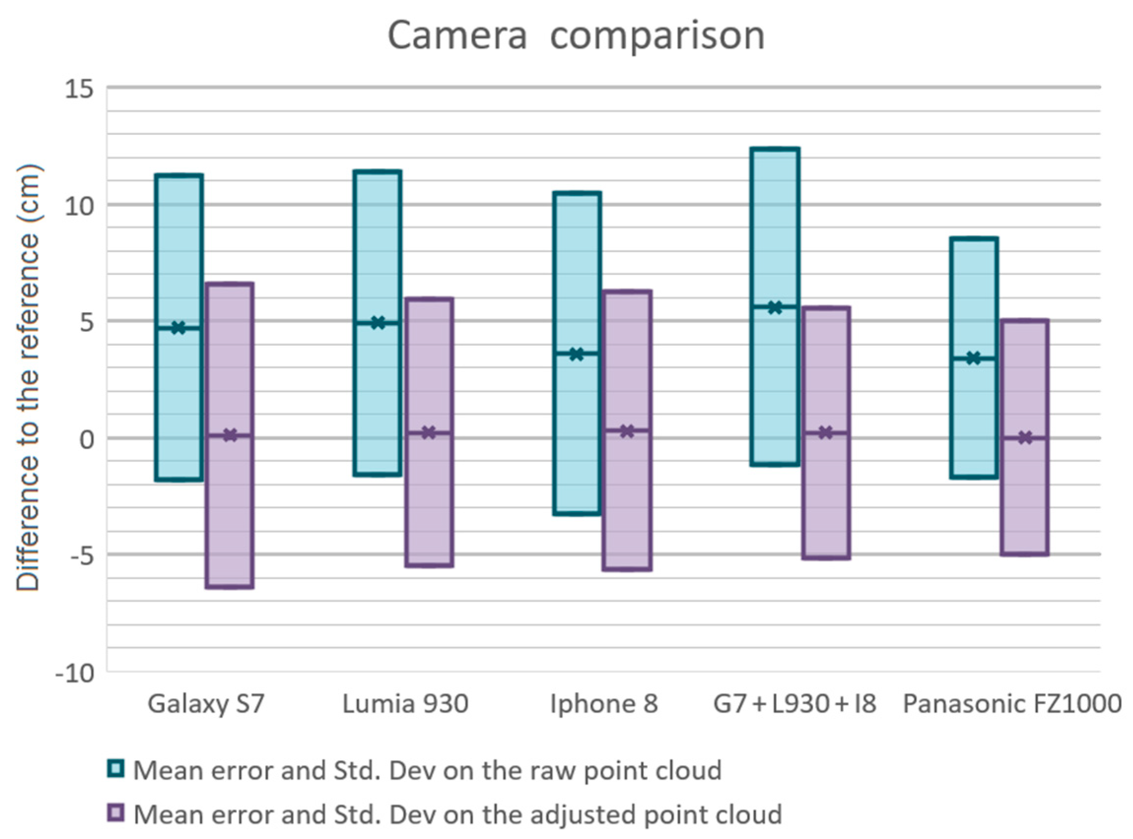
Smartphone SfM photogrammetry has the potential to provide morphological surveys with the same order of quality (in resolution and accuracy) as TLS surveys or photogrammetric surveys using more “classical” cameras (here, a Panasonic Fz1000 bridge camera). This type of terrestrial photogrammetric survey is quicker than a TLS survey (around 20 min against 45 min/scan position) and uses equipment that is less costly (~100 to 200 times cheaper than a TLS), less cumbersome, and more adaptable to weather conditions (particularly wind). We found that the reconstruction quality is not dependent on the smartphone model used and so on its focal length and resolution (as a reminder, the tested smartphones have at least 12 Mpix cameras). We can notice that for photogrammetric purposes, the Lumia 930 provided similar results to the Galaxy S7 and iPhone 8, while it costs two or three times less. Furthermore, considering the order of magnitude of the errors and standard deviations, it is necessary to keep in mind that the TLS mesh used as reference is also affected by errors, for instance due to georeferencing, interpolation in occluded and low-density areas. These errors can vary (i) temporally, from one survey to another, depending for example on RTK DGPS accuracy; and (ii) spatially, depending on the laser angle of incidence, the presence of occluding elements and surface roughness [24]. At Porsmilin site, the errors in TLS data ranged from around 2 cm to 10 cm. It is therefore difficult to discriminate if the differences measured between smartphone SfM point clouds and the TLS mesh are due to the SfM point cloud, the TLS mesh or, more probably, a combination of both. The standard deviations between the SfM point cloud and the TLS mesh can consequently reflect differences in the reconstruction of complex geometries as found on a rocky cliff face. Some parts of the cliff are also vegetated with small bushes, which are challenging for remote sensing methods and can create differences depending on the survey method used and the geometry of data collection.

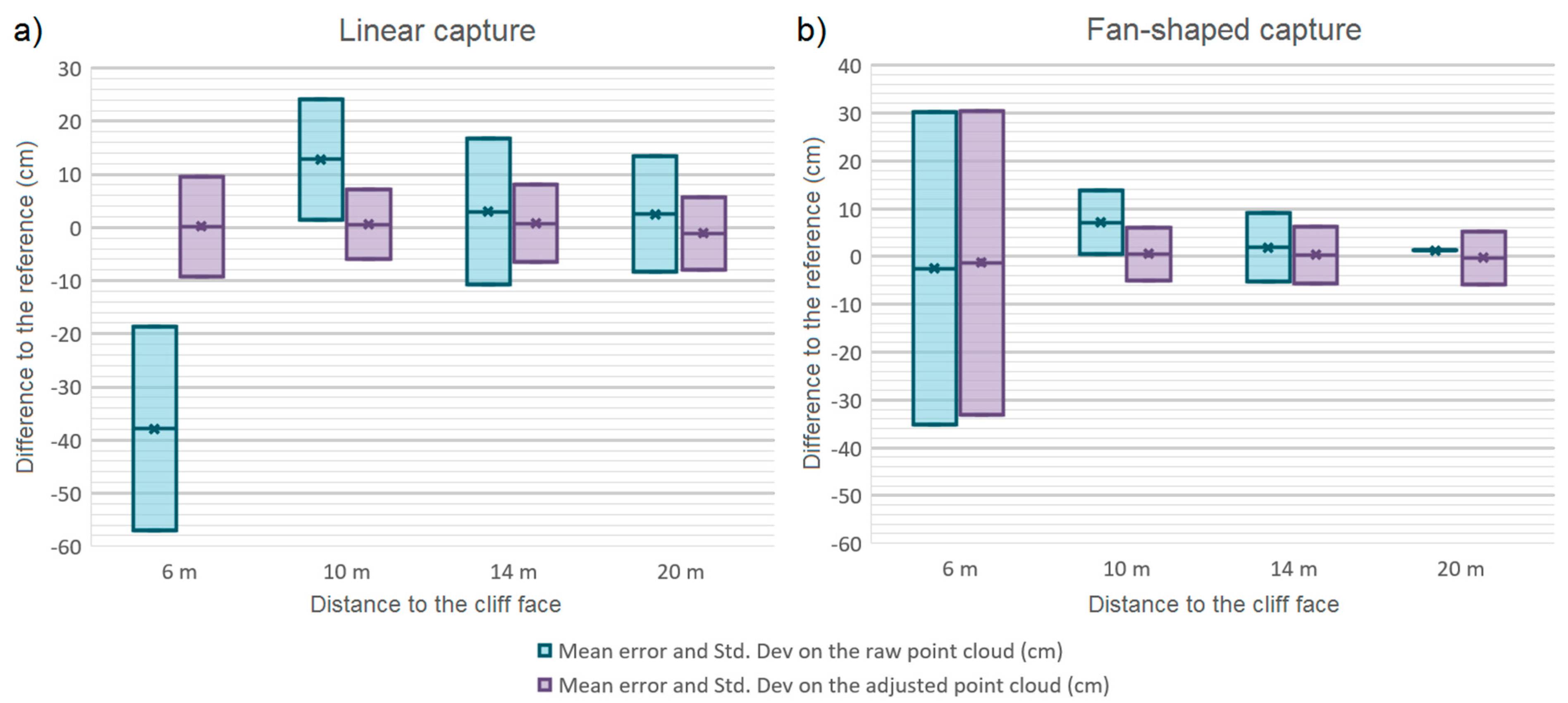
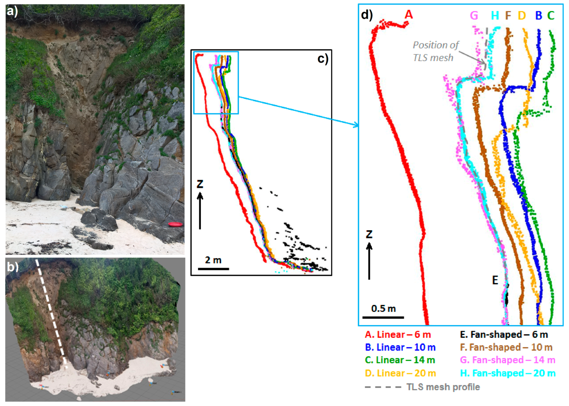
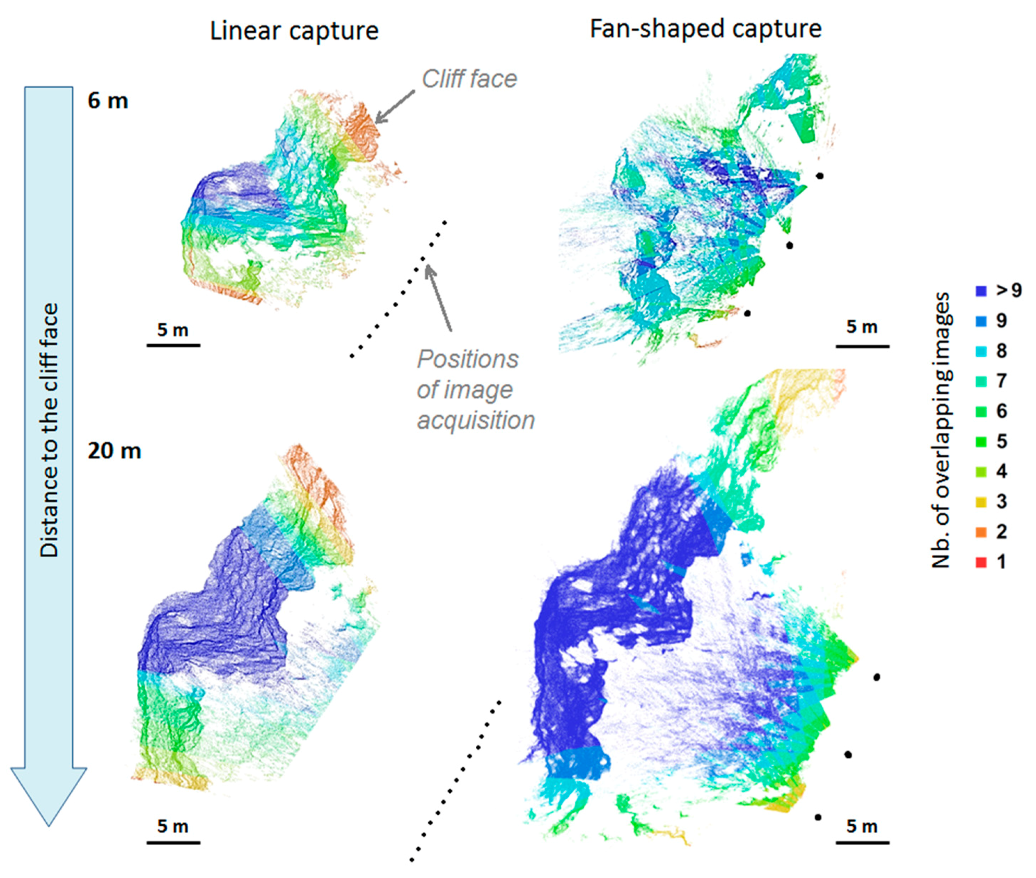
Comparison of the survey protocols shows that point cloud density and reconstruction quality (Table 3 and Figure 7) are closely linked to the configuration of image overlaps. As the distance to the cliff face increases, the image resolution decreases, which may impact tie point identification, but in parallel, the image footprint increases. This increase in image footprint means a larger coverage for the same survey duration (Figure 10) and increased image overlaps, which are favorable to reduce geometrical ambiguities and to limit geometrical distortions. For fan-shaped capturing mode, and at short distances, the image overlap is more homogeneous than for linear capturing mode, but this overlap is low for the imaged area (Figure 10). With increasing distances from the cliff face, fan-shaped capturing mode produces larger image overlaps due to the convergence of images from the different viewpoints. The operator should seek the appropriate distance from the cliff face, offering the optimum trade-off between image footprint (and image overlap) and image resolution. For cliff face reconstruction, fan-shaped capturing mode allows quicker in situ surveys and better results than linear capturing mode provided that the distance to the cliff face is sufficient to ensure a good image overlap.

To a certain extent, the quality of the topographic reconstruction depends on the surveyed environment, including but not limited to the distance to the area of interest, angle of incidence of the line of sight, surface roughness, surface reflectance, and feasibility of GCP deployment. Comparison of our results to the existing literature on smartphone photogrammetry is therefore limited to first order comparison. The quality of the reconstruction obtained on the cliff face is similar to the results obtained in other studies employing comparable methods. The most similar studies to cliff face monitoring concern river or channel banks. Micheletti et al. [23] achieved a mean error of 2.07 cm surveying alpine river banks with iPhone4® photographs at close-range (10 m or less) processed with 123D Catch®, while Prosdocimi et al. [24] obtained a 10 cm gridded DEM of channel banks, with 5.7 cm of RMS error, using iPhone5® photographs processed with Agisoft Photoscan®.

6.2. Beach Reconstruction

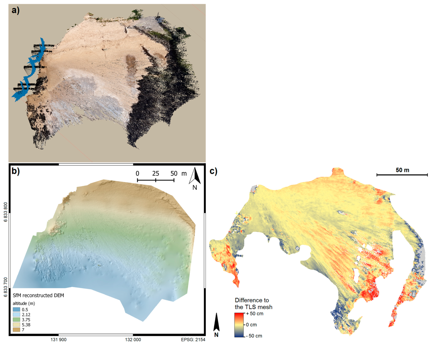
The use of smartphone SfM photogrammetry for beach reconstruction differs from previous studies. The main difficulty is to capture photographs with sufficiently high-angle shots from overlooking points of view. In Porsmilin, the only suitable positions for image acquisition were situated atop the western cliff, which implies that for distant parts of the study area, pixels are more distorted and GCPs are harder to detect (loss of resolution and increase in pixel deformation). As shown in Figure 9c, measurement error is related to the geometry of acquisition, with error increasing along the lines of sight. The absence of GCPs combined with a tangential line of sight are conducive to geometric distortions. These distortions are probably the reason for errors on the perimeter of the study area. Furthermore, the method of error calculation (cloud-to-mesh distance in CloudCompare) only computes Z (i.e., vertical) differences, even though the appearance of the SfM point cloud suggests that there are also some XY (i.e., horizontal) errors, particularly in the eastern part of the study area. Unfortunately, as the targets could not be detected in this area, the XY error is difficult to assess. Furthermore, we can hypothesize that, in the case of a beach survey with tangential lines of sight and a great depth of field, a linear capture mode would provide lower pixel deformation and skewness, and hence better tie point detection.

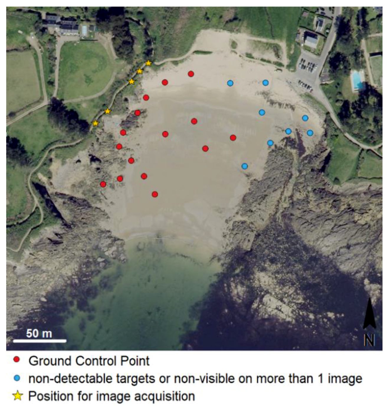
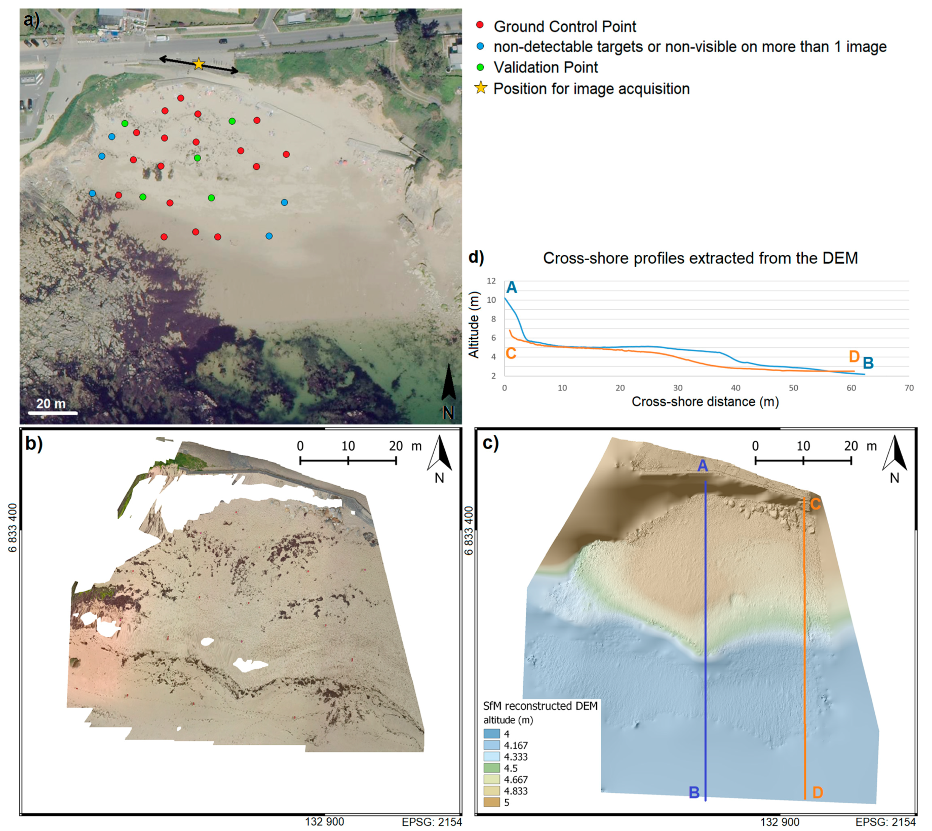
To complement this study and to confirm the importance of having as high-angle shots as possible to improve the quality of the reconstruction, beach survey was tested over another beach site, 1 km to the east, Trégana Beach (Figure 1). This site was chosen as it presents a 30 m long esplanade, situated approximately 12 m above the beach, which offers easy-access favorable points of view for photograph acquisition (Figure 11a). Thirty-five photographs were collected with a linear capture mode using the Lumia 930. No TLS validation data are available for this site. Some targets were used as validation points. This method of error assessment is pointwise, and hence spatially limited; however, it enables to account for both horizontal and vertical errors. Seventeen GCPs and five validation points (Figure 11a) were used. The computed DEM and orthophotograph (Figure 11b,c) have spatial resolutions of 1.0 cm and 0.5 cm, respectively. The XYZ Root Mean Square (RMS) error for the five validation points is estimated to be 1.8 cm. As shown in Figure 11c, the SfM reconstruction not only succeeded in reproducing first order topography, but also complex morphological features such as beach cusps and rocks on the upper beach face.

Smartphone SfM-photogrammetry for beach survey is thus dependent on the site configuration and on the point(s) of view overlooking the study area. As far as possible, it has to be performed with high-angle shots, and at low tide, to maximize the size of the study area and with illumination conditions minimizing sunglint.

6.3. Perspective for Participatory Science Projects

Citizen Observatories can be defined as community-based environmental monitoring and information systems, generally based on citizens’ own devices (e.g. smartphones, laptops, tablets) and social media. This approach aims to increase in situ observations and monitoring capabilities, allowing for example to increase measurement frequency and the number of study sites. Collecting smartphone photographs for SfM reconstruction would thus have a great potential in a participatory science projects.

Obtaining satisfactory results regardless of the smartphone model used and when mixing photographs from different smartphones is particularly promising if we aim to apply these methods in citizen observatories. Indeed, photographs collected by different people (potentially equipped with different devices) could be used in the same SfM reconstruction process. Future work will be dedicated to develop a mobile app and to test the concept among citizens.

Nevertheless, in such participatory monitoring frameworks, the RTK DGPS measurement of targets used as GCPs would be an issue. Coastal environments are highly dynamic, and to limit error propagation in sedimentary budgets a suitable monitoring strategy requires high resolution and high accuracy surveys. Consequently, using geotagged photographs only may not provide a sufficient accuracy. For cliff monitoring, the problem can be overcome by implementing fixed targets on the rock wall. On beaches, the problem persists, unless there are some unmoving visible rocks or boulders.

7. Conclusions

This study has demonstrated that smartphone SfM photogrammetry has a real potential for coastal monitoring. Centimetric accuracy in SfM point clouds can be achieved, regardless of the smartphone model used, and when mixing photographs from different smartphones. The results obtained are similar to those obtained using TLS. Fan-shaped capturing mode allows quicker in situ surveys and produces better results than linear capturing mode provided that the distance to the cliff face is sufficient to ensure a good image overlap. High-angle shots are preferable to achieve satisfactory results over beaches, which may limit application of the method for certain sites.

A larger uptake of smartphone SfM photogrammetry is expected with the emergence of citizen observatories. This will require adapting the survey protocols in order to make them usable by a large number of people.

References

1. Splinter, K.; Harley, M.; Turner, I. Remote Sensing is changing our view of the coast: Insights from 40 years of monitoring at Narrabeen-Collaroy, Australia. Remote Sens. 2018, 10, 1744. [Google Scholar] [CrossRef]
2. Baily, B.; Nowell, D. Techniques for monitoring coastal change: A review and case study. Ocean Coast. Manag. 1996, 32, 85–95. [Google Scholar] [CrossRef]
3. Baptista, P.; Bastos, L.; Bernardes, C.; Cunha, T.; Dias, J. Monitoring Sandy Shores Morphologies by DGPS—A Practical Tool to Generate Digital Elevation Models. J. Coast. Res. 2008, 246, 1516–1528. [Google Scholar] [CrossRef]
4. Suanez, S.; Cariolet, J.-M.; Cancouët, R.; Ardhuin, F.; Delacourt, C. Dune recovery after storm erosion on a high-energy beach: Vougot Beach, Brittany (France). Geomorphology 2012, 139, 16–33. [Google Scholar] [CrossRef]
5. Aarninkhof, S.G.J.; Turner, I.L.; Dronkers, T.D.T.; Caljouw, M.; Nipius, L. A video-based technique for mapping intertidal beach bathymetry. Coast. Eng. 2003, 49, 275–289. [Google Scholar] [CrossRef]
6. Holman, R.A.; Stanley, J. The History and Technical Capabilities of Argus. Coast. Eng. 2007, 54, 477–491. [Google Scholar] [CrossRef]
7. Turki, I.; Medina, R.; Gonzalez, M.; Coco, G. Natural variability of shoreline position: Observations at three pocket beaches. Mar. Geol. 2013, 338, 76–89. [Google Scholar] [CrossRef]
8. Andriolo, U.; Sánchez-García, E.; Taborda, R. Operational Use of Surfcam Online Streaming Images for Coast. Morphodynamic Studies. Remote Sens. 2019, 11, 78. [Google Scholar] [CrossRef]
9. Jaud, M.; Letortu, P.; Augereau, E.; Le Dantec, N.; Beauverger, M.; Cuq, V.; Prunier, C.; Le Bivic, R.; Delacourt, C. Adequacy of pseudo-direct georeferencing of terrestrial laser scanning data for coastal landscape surveying against indirect georeferencing. Eur. J. Remote Sens. 2017, 50, 155–165. [Google Scholar] [CrossRef] [Green Version]
10. Letortu, P.; Costa, S.; Maquaire, O.; Delacourt, C.; Augereau, E.; Davidson, R.; Suanez, S.; Nabucet, J. Retreat Rates, Modalities and Agents Responsible for Erosion along the Coast. Chalk Cliffs of Upper Normandy: The Contribution of Terrestrial Laser Scanning. Geomorphology 2015, 245, 3–14. [Google Scholar] [CrossRef]
11. Fabbri, S.; Giambastiani, B.M.S.; Sistilli, F.; Scarelli, F.; Gabbianelli, G. Geomorphological Analysis and Classification of Foredune Ridges Based on Terrestrial Laser Scanning (TLS) Technology. Geomorphology 2017, 295, 436–451. [Google Scholar] [CrossRef]
12. Delacourt, C.; Allemand, P.; Jaud, M.; Grandjean, P.; Deschamps, A.; Ammann, J.; Cuq, V.; Suanez, S. DRELIO: An unmanned helicopter for imaging coastal area. J. Coast. Res. 2009, 56, 1489–1493. [Google Scholar]
13. Turner, I.L.; Harley, M.D.; Drummond, C.D. UAVs for coastal surveying. Coast. Eng. 2016, 114, 19–24. [Google Scholar] [CrossRef]
14. Jaud, M.; Delacourt, C.; Le Dantec, N.; Allemand, P.; Ammann, J.; Grandjean, P.; Nouaille, H.; Prunier, C.; Cuq, V.; Augereau, E.; et al. Diachronic UAV Photogrammetry of a Sandy Beach in Brittany (France) for a Long-Term Coast. Observatory. ISPRS Int. J. Geo-Inf. 2019, 8, 267. [Google Scholar] [CrossRef]
15. Stéphan, P.; Suanez, S.; Fichaut, B.; Autret, R.; Blaise, E.; Houron, J.; Ammann, J.; Grandjean, P. Monitoring the medium-term retreat of a gravel spit barrier and management strategies, Sillon de Talbert (North Brittany, France). Ocean Coast. Manag. 2018, 158, 64–82. [Google Scholar]
16. Lim, M.; Petley, D.N.; Rosser, N.J.; Allison, R.J.; Long, A.J.; Pybus, D. Combined Digital Photogrammetry and Time-of-Flight Laser Scanning for Monitoring Cliff Evolution. Photogramm. Rec. 2005, 20, 109–129. [Google Scholar] [CrossRef]
17. Letortu, P.; Jaud, M.; Grandjean, P.; Ammann, J.; Costa, S.; Maquaire, O.; Davidson, R.; Le Dantec, N.; Delacourt, C. Examining high-resolution survey methods for monitoring cliff erosion at an operational scale. GISci. Remote Sens. 2017, 55, 457–476. [Google Scholar] [CrossRef]
18. Medjkane, M.; Maquaire, O.; Costa, S.; Roulland, T.; Letortu, P.; Fauchard, C.; Antoine, R.; Davidson, R. High-resolution monitoring of complex coastal morphology changes: Cross-efficiency of SfM and TLS-based survey (Vaches-Noires cliffs, Normandy, France). Landslides 2018, 15, 1097–1108. [Google Scholar] [CrossRef]
19. James, M.R.; Robson, S. Straightforward reconstruction of 3D surfaces and topography with a camera: Accuracy and geoscience application. J. Geophys. Res. 2012, 117. [Google Scholar] [CrossRef] [Green Version]
20. Harley, M.D.; Kinsela, M.A.; Sánchez-García, E.; Vos, K. Shoreline Change Mapping Using Crowd-Sourced Smartphone Images. Coast. Eng. 2019, 150, 175–189. [Google Scholar] [CrossRef]
21. Al-Hamad, A.; El-Sheimy, N. Smartphones Based Mobile Mapping Systems. Int. Arch. Photogramm. Remote Sens. Spat. Inf. Sci. 2014, 29–34. [Google Scholar] [CrossRef]
22. Kim, J.; Lee, S.; Ahn, H.; Seo, D.; Park, S.; Choi, C. Feasibility of employing a smartphone as the payload in a photogrammetric UAV system. ISPRS J. Photogramm. Remote Sens. 2013, 79, 1–18. [Google Scholar] [CrossRef]
23. Micheletti, N.; Chandler, J.H.; Lane, S.N. Investigating the geomorphological potential of freely available and accessible structure-from-motion photogrammetry using a smartphone. Earth Surf. Process. Landf. 2015, 40, 473–486. [Google Scholar] [CrossRef]
24. Prosdocimi, M.; Calligaro, S.; Sofia, G.; Dalla Fontana, G.; Tarolli, P. Bank erosion in agricultural drainage networks: New challenges from structure-from-motion photogrammetry for post-event analysis: SfM for Post-Event Analysis. Earth Surf. Process. Landf. 2015, 40, 1891–1906. [Google Scholar] [CrossRef]
25. Ozturk, H.S.; Kocaman, S.; Gokceoglu, C. A low-cost approach for determination of discontinuity orientation using smartphone images and application to a part of Ihlara Valley (Central Turkey). Eng. Geol. 2019, 254, 63–75. [Google Scholar] [CrossRef]
26. Kazhdan, M.; Bolitho, M.; Hoppe, H. Poisson Surface Reconstruction. In Proceedings of the Symposium on Geometry Processing, Cagliari, Sardinia, Italy, 26–28 June 2006; pp. 61–70. [Google Scholar]
Figure 1. (a) Localization of Porsmilin beach and (b) surrounding cliffs at the entrance of the Bay of Brest in Brittany, France.
Remotesensing 11 02242 g001
Figure 2. Comparison of photographs taken by the smartphones (Galaxy S7, Lumia 930 and iPhone 8) and the Fz1000 bridge camera. The size of the photographs is proportional to their native pixel size.
Remotesensing 11 02242 g002
Figure 3. (a) Studied portion of the Porsmilin western cliff face and configuration of the Ground Control Points (GCPs) for the comparison of the different smartphones. (b) Example of target used as GCP.
Remotesensing 11 02242 g003
Figure 4. Operational mode for the second test on Porsmilin cliff (left of the image). (a) Position of the GCPs and of the segments A, B, C and D at respectively 6 m, 10 m, 14 m and 20 m from the cliff foot. (b), (c) Geometry of the shot modes tested along each segment, with linear capture (b) or fan-shaped capture (c).
Remotesensing 11 02242 g004
Figure 5. Configuration of the Porsmilin Beach survey by smartphone Structure-from-Motion (SfM) photogrammetry, using the Galaxy S7® (Background image: BD Ortho—IGN©).
Remotesensing 11 02242 g005
Figure 6. Mean error and standard deviation for the SfM point clouds resulting from the different cameras compared to the Terrestrial Laser Scanner (TLS) mesh.
Remotesensing 11 02242 g006
Figure 7. Mean error and standard deviation for the SfM point clouds resulting from the different survey protocols compared to the TLS mesh. (a) Linear capture, (b) Fan-shaped capture.
Remotesensing 11 02242 g007
Figure 8. (a) Picture of the cliff face at the moment of the survey. (b) Position of the topographic profile on the SfM dense point cloud. (c,d) Comparison of shape and position of the profiles extracted from the SfM dense point cloud obtained for the different survey protocols.
Remotesensing 11 02242 g008
Figure 9. (a) SfM dense point cloud obtained in Porsmilin Beach from 5 capturing positions at the top of the western cliff (survey using Galaxy S7). (b) Porsmilin Digital Elevation Model (DEM) obtained from the point cloud. (c) Spatial distribution of the difference between the SfM point cloud and the TLS mesh.
Remotesensing 11 02242 g009
Figure 10. Impact of the survey protocol (capturing mode and distance) on the image overlap.
Remotesensing 11 02242 g010
Figure 11. (a) Configuration of the Trégana Beach survey by smartphone SfM photogrammetry, using the Lumia 930 (Background image: BD Ortho—IGN©). Orthophotograph (b) and DEM (c) obtained by SfM processing. (d) Cross-shore profiles extracted from the smartphone photogrammetric DEM.
Remotesensing 11 02242 g011