Multi-Temporal Monsoon Crop Biomass Estimation Using Hyperspectral Imaging

Abstract

Hyperspectral remote sensing is considered to be an effective tool in crop monitoring and estimation of biomass. Many of the previous approaches are from single year or single date measurements, even though the complete crop growth with multiple years would be required for an appropriate estimation of biomass. The aim of this study was to estimate the fresh matter biomass (FMB) by terrestrial hyperspectral imaging of the three crops (lablab, maize and finger millet) under different levels of nitrogen fertiliser and water supply. Further, the importance of the different spectral regions for the estimation of FMB was assessed. The study was conducted in two experimental layouts (rainfed (R) and irrigated (I)) at the University of Agricultural Sciences, Bengaluru, India. Spectral images and the FMB were collected over three years (2016–2018) during the growing season of the crops. Random forest regression method was applied to build FMB models. R² validation (R²_val) and relative root mean square error prediction (rRMSEP) was used to evaluate the FMB models. The Generalised model (combination of R and I data) performed better for lablab (R²_val = 0.53, rRMSEP = 13.9%), maize (R²_val = 0.53, rRMSEP = 18.7%) and finger millet (R²_val = 0.46, rRMSEP = 18%) than the separate FMB models for R and I. In the best derived model, the most important variables contributing to the estimation of biomass were in the wavelength ranges of 546–910 nm (lablab), 750–794 nm (maize) and 686–814 nm (finger millet). The deviation of predicted and measured FMB did not differ much among the different levels of N and water supply. However, there was a trend of overestimation at the initial stage and underestimation at the later stages of crop growth.

1. Introduction

The majority of India’s population (60%) depends on the agricultural sector for their livelihood [1]. Agriculture depends mainly on monsoon rainfall, surface water and ground water irrigation. Since the variability of monsoon rainfall is high, it forces the south Indian farmers to adapt their irrigated areas to local water availability [2]. Irrigated crop production is a major contributor to the green revolution, which has enabled the country to be self-sufficient [3], accompanied by fertiliser application and other inputs in semi-arid parts of India. Timely fertiliser application with water supply is essential for a successful crop. Spectral data from Remote Sensing (RS) have been studied for many years for an adequate assessment of nutrient and water variability for yield optimisation [4,5,6]

RS can be an effective tool in monitoring crop production [7,8,9] and estimating yield [10,11]. Early estimation of yield may allow better planning and forecasting the market prices and support food security based on the regional, national and global demand and supply. RS allows collecting information about crop production using non-destructive methods [12] on a large scale for many fields at the same time. Hyperspectral (HS) RS provides continuous narrow spectral data from 400 to 2500 nm and have been proved to capture the variations in spectral response of the crop for the detection of nitrogen (N) content [13,14], biomass [15] and water stress [6,16]. Development of HS sensors and their application in estimating crop biomass from multi-year data [17] has gained increasing attention in the recent years. Multi-temporal images provide more information on vegetation phenology under wet and dry conditions than a single image [18]. Many studies related to multi-temporal hyperspectral imaging have been published on crops such as rice (Oryza sativa L.) [19], wheat (Triticum aestivum L.) [20,21] and maize (Zea mays L.) [10]. Besides maize, lablab (Lablab purpureus L.) and finger millet (Eleusine coracana L.) are primary crops in the semi-arid region of South India. The state of Karnataka generates the major share of lablab (90%) [22] and finger millet (62.01%) [23] production of India. However, well-defined multi-year studies on the estimation of biomass for maize, lablab and finger millet using multi-temporal hyperspectral data under varying nitrogen (N) fertiliser and water supply levels are still lacking.

The aim of this study was to assess the potential of terrestrial hyperspectral imaging for the estimation of monsoon crop biomass based on data from three years (2016–2018). The specific objectives of the study were: (1) to develop statistical models to predict the fresh matter biomass (FMB) of the three crops: lablab, maize and finger millet; (2) to assess the effect of different levels of N and water supply on the predicted FMB value and for a wide range of crop phenology over the complete growing period; and (3) to evaluate the importance of spectral regions in the resulting models and understand the causal relationships of the model.

2. Materials and Methods

The study was conducted during 2016–2018 at GKVK campus of University of Agricultural Sciences, Bengaluru (UASB) located in the eastern dry zone of Karnataka state, India (12°58′20.79′′N, 77°34′50.31′′E, 920 m.a.s.l) (Figure 1a). The soils of the study area are formed by Kandic Paleustalfs and Dystric Nitisols as dominant soil types and the climate is described as tropical savanna climate with the rainy season from June to October. The mean annual temperature is 29.2 °C with an average precipitation of 923 mm [24]. The total rainfall and mean temperature data of the monsoon cropping season varied from 2016 to 2018 (

Table 1. Total rainfall and mean temperature data of the cropping seasons.

Years	2016	2017	2018
Rainfall (mm)	403.4	763.2	264.8
Temperature (°C)	23.51	23.48	23.28

) [25].

2.1. Experimental Site

Two experiments were established with different irrigation regimes: rainfed (R) and drip irrigated (I). Each year has two cropping seasons, namely rainy/monsoon season (July–November) and dry season (February–May). Even in the monsoon season, drip irrigation systems are common, as the southwest monsoons are getting increasingly unreliable and timely irrigation enhances the crop productivity. In the rainy season, lablab (cultivars: HA 4 and HA 3), maize (cultivars: Nithyashree and NAH 1137) and finger millet (cultivars: GPU-28, MR-6 and ML-365) were cultivated in both experiments (

Table A1. Varietal description of the crops lablab, maize and finger millet grown in three years.

Crops	Years Grown	Varieties	Sowing	Duration (days)	Yield (t/ha)		Salient Features
					Rainfed	Irrigated
Lablab	2016 and 2017	HA 4 (HA 3 xMagadi local)	Can be grown throughout the year as they are photo insensitive	100–105	Dry Seeds: 1–1.2, Green pods: 4.5–5		Pods are constricted with characteristic odour (Sogadu) in all the three cropping seasons
	2018	HA 3 (HA 1 × US 67-31)		95–100	Dry Seeds: 0.8–0.9 Green pods: 4.5–5		Flat pods with no odour (Sogadu)
Maize	2016 and 2017	Nithyashree (SKV-50 × NA1-105)	Can be grown throughout the year	110–120	Grain: 7.41–7.90 Straw: 19.77	Grain: 7.90–8.40 Straw: 29.65	Tolerant to downy mildew, leaf blight and stem borer
	2018	NAH 1137 (Hema)		110–120	Grain: 7.90–8.40 Straw: 19.77	Grain: 8.89–9.39 Straw: 29.65
Finger millet	2016	GPU-28 (Indaf 5 × (Indaf 9 × IE 1012))	July–August	110–115	Average Grain: 3.5–4		Medium tall plants, semi compact ears with tip incurved fingers. Highly resistant to finger and neck blast
	2017	MR-6 (African white × RoH 2)	June–July	120–125	Average Grain: 3–3.5		100–110 cm tall plants, open ears with tip incurved fingers
	2018	ML-365 (IE 1012 × Indaf 5)	June–August (Kharif monsoon) January–February (Rabi dry)	110–115	Average Grain: 5–5.5		Medium height, semi compact ears with tip incurved fingers. Resistant to neck blast and tolerant to drought

) [26,27,28,29,30]. The fertiliser application was done by broadcasting at three levels to all crops. At high levels, the complete 100% application of N (recommended dosage) was applied and a reduced amount was applied at medium and low levels, which varied across the years. To lablab, the complete N dosage was applied at the time of sowing and for maize and finger millet it was split into two halves, i.e. at the time of sowing and four weeks after sowing (top dressing) with the objective of supplying nitrogen to growing plants in the readily available form and avoid leaching losses by heavy rainfalls, which frequently occur after sowing. Phosphorous and potassium were applied completely to all crops at the time of sowing (

Table A2. Nitrogen (N), phosphorous (P₂O₅) and potassium (K₂O) application rates to lablab, maize and finger millet crops in rainfed (R) and irrigated (I) experiments during 2016–2018.

Mineral Fertilisation	Lablab						Maize						Finger Millet
	2016		2017		2018		2016		2017		2018		2016		2017		2018
	R	I	R	I	R	I	R	I	R	I	R	I	R	I	R	I	R	I
N (kg ha−1) §	25	25	25	25	25	25	100	150	100	150	150	150	50	100	50	100	50	50
P2O5 (kg ha−1)	10	10	50	50	10	10	50	75	50	75	50	75	40	50	40	50	40	50
K2O (kg ha−1)	10	10	25	25	10	10	37.5	50	25	40	37.5	50	37.5	50	37.5	50	37.5	50

§ Recommended application rate (referred to as high in Figure 1); averaged across years, medium application rates were 53.3%, 56.2% and 58.3% from the high level for lablab, maize and finger millet, respectively; low application rates in 2016 were 40.0%, 41.7% and 50.0% from the high level for lablab, maize and finger millet, respectively, and zero application was done in 2017 and 2018.

).

Each block of a particular crop had three experimental plots (6 m × 12 m) with three N levels (low, medium and high) distributed in a randomised block design (Figure 1). In this split plot experiment, each plot was subdivided into two sub plots (6 m each), one was used for destructive biomass sampling (S) and the other one was used for non-destructive spectral measurements (H). In total, 36 plots (3 crops × 4 blocks × 3 fertiliser levels) were used for the spectral and biomass sampling (Figure 1).

2.2. Spectral Data Measurements

Three hyperspectral images were taken in each H subplot using the full-frame hyperspectral camera UHD 185-Firefly [31] mounted on a terrestrial tripod. The distance between the camera and the plant canopy height was 1.5 m throughout the growth of the crop to cover the same area of approximately 1 m² in all images. The camera measured the spectral range from 450 to 998 nm, of which the wavelength between 470 and 950 nm was further analysed, as the signal-to-noise ratio was too low for the wavebands from 450 to 470 and 950 to 998 nm. The spectral range was divided into 121 bands with a band width of 4 nm. The focal length of the camera was 12.1 mm with the image size of 50 × 50 pixels covering the area of 1 m × 1 m at the applied height (2 cm spatial resolution). Prior to the measurement, the camera was calibrated using a dark (cap covering the lens) and white reflectance plane (95% reflectance Zenith Lite) [32] to calculate reflectance directly from the measured radiance. Although light conditions varied throughout the three years due to different illumination angles, the goal was to keep it as constant as possible. During the calibration in the field, the integration time was automatically obtained. The spectral reflectance of each pixel was normalised by dividing with the maximum reflectance value of the same pixel to reduce temporal variation and random noise [33].

Each image contained non-vegetation elements such as soil, drip irrigation pipes and shadows. To reduce the effect of these elements, a two-step procedure was applied (Figure 2). First, the Normalised Difference Vegetation Index (NDVI) [8] was calculated as the difference between reflectance in the red (620–750 nm) and near-infrared (NIR) (750–1400 nm), divided by the sum of reflectance in the red and NIR spectral range. Second, a two-class k-means clustering algorithm was applied to separate vegetation and non-vegetation using the NDVI values. The two class centroids were identified based on NDVI values in such a way that the distance between the centroids were minimised. Finally, only the pixels classified as vegetation were used to calculate the average spectral reflectance for each image. The three images collected in each plot were averaged resulting in one spectral reflectance curve per H subplot and sampling date.

2.3. Biomass Sampling

The fresh matter weight of 2–4 plants were measured in the field and extrapolated to 1 m². The maximum number of samples collected for a particular crop type in a particular growing season was 60 (5 sampling dates × 3 fertiliser treatments × 4 replicates), but the number of sampling varied among the three years (

Table 2. Total number of samples from rainfed (R) and irrigated (I) experiments.

Experiments	Number of Samples in R			Number of Samples in I
Year	2016	2017	2018	2016	2017	2018
Lablab	60	60	12	52	60	12
Maize	48	48	12	60	48	12
Finger millet	60	36	12	52	36	12
Total annual crop-wise	168	144	36	164	144	36
Total experiment-wise	348			344
Grand total	692

).

2.4. Sampling Dates

In 2016 (Y1), the sampling was done on five sampling dates (Y1S1–Y1S5) in both irrigation regimes (R and I) for the three crops. Rainfed maize at the final sampling date in 2016 (Y1S5) was not sampled due to technical difficulties with the sensor. In 2017 (Y2), there were five sampling dates (Y2S1–Y2S5) for lablab, four for maize (Y2S1–Y2S4) and three for finger millet (Y2S1–Y2S3) in both irrigation regimes (R and I). In Y2, irrigated maize top-dressing fertilisation was mixed up for a few low, medium and high plots and hence the plots I07, I08, I09, I13, I14, and I15 (Figure 1c) were eliminated from analysis for Sampling dates 2–4 (Y2S2–Y2S4). In 2018 (Y3), there was one sampling date (Y3S1) for all three crops. Assessment of phenological stages of the crop was carried out by recording the morphological characteristics of the plants according to Biologische Bundesanstalt, Bundessortenamt und Chemische Industrie (BBCH) [34]. In total, there were 11 sampling dates (BBCH 1–8) for 2016–2018 (

Table A3. Phenological stages of lablab, maize and finger millet at the sampling dates in rainfed and irrigated experiment from 2016 to 2018 (BBCH scale).

Rainfed Experiment
Sampling Dates	Lablab (BBCH/DAS*)			Maize (BBCH/DAS*)			Finger Millet (BBCH/DAS*)
	2016	2017	2018	2016	2017	2018	2016	2017	2018
1	2/40	2/23		3/42	1/25		2/44	2/30
2	5/53	2/38		5/61	3/45		3/65	3/52
3	6/63	5/47		7/81	6/67	7/79	5/94	5/81	5/79
4	7/73	6/69	7/78	8/98	7/108		7/109
5	8/89	8/89					8/126
Irrigated experiment
1	2/41	2/24		3/43	1/27		2/45	2/32
2	6/56	5/39		5/62	3/46		3/66	3/53
3	7/64	6/48		7/88	6/68	7/87	5/96	5/82	5/87
4	7/74	7/72		7/100	7/110		7/110
5	8/97	8/90	8/83	8/128			8/135

* DAS, Days after Sowing. BBCH: 1: Leaf development; 2: Formation of side shoots/tillering; 3: Stem elongation; 5: Inflorescence emergence; 6: Flowering; 7: Development of fruit; 8: Ripening

).

2.5. Statistical Analysis

To predict the fresh matter biomass (FMB) from reflectance data, machine learning random forest regression (RFR) in caret package [35] was used [36]. Although RFR does not require normal distribution of the FMB dataset, the original dataset was skewed towards one side. Hence, the FMB measured in the S subplots were cube root transformed to assure normal distribution of the dataset. RFR is a regression tree technique, which builds multiple decision trees and ensembles them for an accurate prediction [36]. It is less sensitive to overfitting as the subsets are drawn randomly each time. The regression trees has the ability to deal with complex relationships between variables for large datasets [37]. Each crop was modelled separately for R and I experiment based on three years datasets (6 models). Further, the datasets from both irrigation regimes on each crop were combined to give one Generalised model to check the robustness of the model independent of water supply. To eliminate the bias involved in splitting the data into training and testing sets, 100 different random subsets (75% for training and 25% for testing) were generated based on the sampling dates for each crop separately. Using these random subsets, 100 RFR models were calibrated and validated to predict the FMB for each crop from reflectance data. All machine learning methods have specific configuration parameters called tune parameters or hyperparameters, which optimise the performance of the predictive modelling algorithm [38]. For RFR model, two tune parameters need to be determined, i.e. number of trees and mtry. The number of trees parameter was always kept to a default value of 500 and the mtry parameter value was tuned using the repeated cross-validation (five-fold, three repeats) procedure. The mtry parameter value was set between 1 and 15 and the optimum mtry parameter for each model was identified. The model estimation accuracy of FMB was evaluated using R² validation (R²_val) (Equation (1)) [39], the root mean square error of prediction (RMSEP) (Equation (2)), and the relative root mean square error prediction (rRMSEP) (Equation (3)).

$$R_{val}^2=\left[1-\frac{{{\displaystyle \sum }}_{i=1}^n{\left(y_i-{\widehat{y}}_i\right)}^2}{{{\displaystyle \sum }}_{i=1}^n{\left(y_i-{\overline{y}}_i\right)}^2}\right]$$

(1)

$$RMSEP=\sqrt{\frac{{{\displaystyle \sum }}_{i=1}^n{\left({\widehat{y}}_i-y_i\right)}^2}{n}}$$

(2)

$$rel.RMSEP=\frac{RMSEP}{\max \left(y_i\right)-\min \left(y_i\right)}$$

(3)

where $y_i$ is the measured fresh matter biomass, ${\widehat{y}}_i$ is the predicted fresh matter biomass, ${\overline{y}}_i$ is the average measured fresh matter biomass, and n is the number of samples.

To determine the important wavelengths in the prediction of FMB, the best model was identified out of 100 FMB models on each crop based on the lowest RMSE value. From the best model, the wavelengths contributing above 75% in the prediction of FMB were identified. The normalised deviation between the predicted and observed FMB values were calculated and differences in the deviation based on N levels, sampling dates and water supply were examined (Equation (4)).

$$Normaliseddeviation=\frac{PredictedFMB-ObservedFMB}{PredictedFMB+ObservedFMB}$$

(4)

3. Results

In the rainfed experiment, the range of FMB (S sub-plot) over the three years 2016–2018 was 0.16–14.6 t/ha for lablab, 0.76–67.71 t/ha for maize and 0.89–59.39 t/ha for finger millet (Figure 3). Similarly, for irrigated experiment, it was 0.22–44.33 t/ha for lablab, 2.28–79.38 t/ha for maize and 0.91–69.63 t/ha for finger millet. Crop growth continuously increased until S3 or S4 and started to decrease at later stages in all crops and along the three years. The FMB was higher in I than R experiment except for finger millet at Y1S1 and Y2S2.

To gain an impression of the spectral variation for each crop, minimum, average and maximum spectral reflectance from the images of rainfed and irrigated experiments were determined for the three crops lablab, maize and finger millet during the three monsoon seasons (Figure 4).

3.1. Crop Specific FMB Models

To develop a prediction model for FMB, which is valid for varying conditions, individual FMB models were developed for two irrigation regimes (i.e., R and I) and a combination of the datasets of both irrigation regimes (i.e., Generalised model). The prediction accuracy of the FMB models varied between the crops and depended on the dataset (R, I, or Generalised) used for model development (Figure 5). The lowest rRMSEP value nearing to zero was considered as a better model. Building the RFR models separately for both R and I treatments, the lowest median rRMSEP for lablab was found in I with 17.9% (R²_val = 0.34) and for maize and finger millet in R experiment with 18.5% (R²_val = 0.60) and 19.8% (R²_val = 0.46), respectively. With the combined dataset, the rRMSEP for lablab was 13.9% (R²_val = 0.53), for finger millet was 18% (R²_val = 0.46) and for maize was 18.7% (R²_val = 0.53). Overall, compared to the experiment-wise modelling approach, model accuracy (in terms of rRMSEP) was higher for all crops when models were built with data from both water supply levels.

In RFR modelling, the mtry parameter indicates the number of input variables randomly chosen at each node. Optimum mtry values (best tune values) were found to be 13, 7 and 7 for lablab; 8, 12 and 13 for maize; and 8, 2 and 7 for finger millet, respectively, for the Rainfed, Irrigated and Generalised models.

The plots of fit for the 100 randomised Generalised models of the three crops are shown in Figure 6. The randomised models were based on stratified (according to sampling date and fertilisation rate) randomly selected samples for the calibration and validation dataset. Having considered these random effects in RFR modelling, it becomes obvious that predictions show a substantial underestimation with increasing FMB values (Figure 6).

3.2. Performance of the Generalised Models Considering N Application Rates, Sampling Dates and Water Supply

The normalised deviation of predicted and measured biomass was used to check if the prediction accuracy of Generalised models varied among the three levels of N application (Figure 7). Overall, only minor deviations were found among low, medium and high levels of N supply for all crops between 2016 and 2018.

Prediction accuracy of Generalised models varied strongly among the sampling dates (Figure 8). While in Y1, normalised deviation for lablab showed an irregular pattern, such as an overestimation (Y1S1 and Y1S3), underestimation (Y1S2) and good concordance (Y1S4 and Y1S5). A decreasing trend of deviation was observed with increasing crop maturity in Y2. With maize, there was a general decline across sampling dates both in Y1 and Y2. With finger millet, there was overestimation for the early sampling dates (Y1S1–Y1S2 and Y2S1–Y2S2) followed by decreasing underestimation for the later sampling dates in 2016 (Y1S3–Y1S5). Following this deviation, it can be concluded that crop phenology influenced model performance with a tendency towards overestimation at early stages and an underestimation at later stages of crop growth.

No systematic over- or underestimation was found for biomass prediction of the three crops at the two levels of water supply (Figure 9). Hence, model prediction was rather robust with slightly larger deviations for lablab at both water supply levels as compared to the other crops.

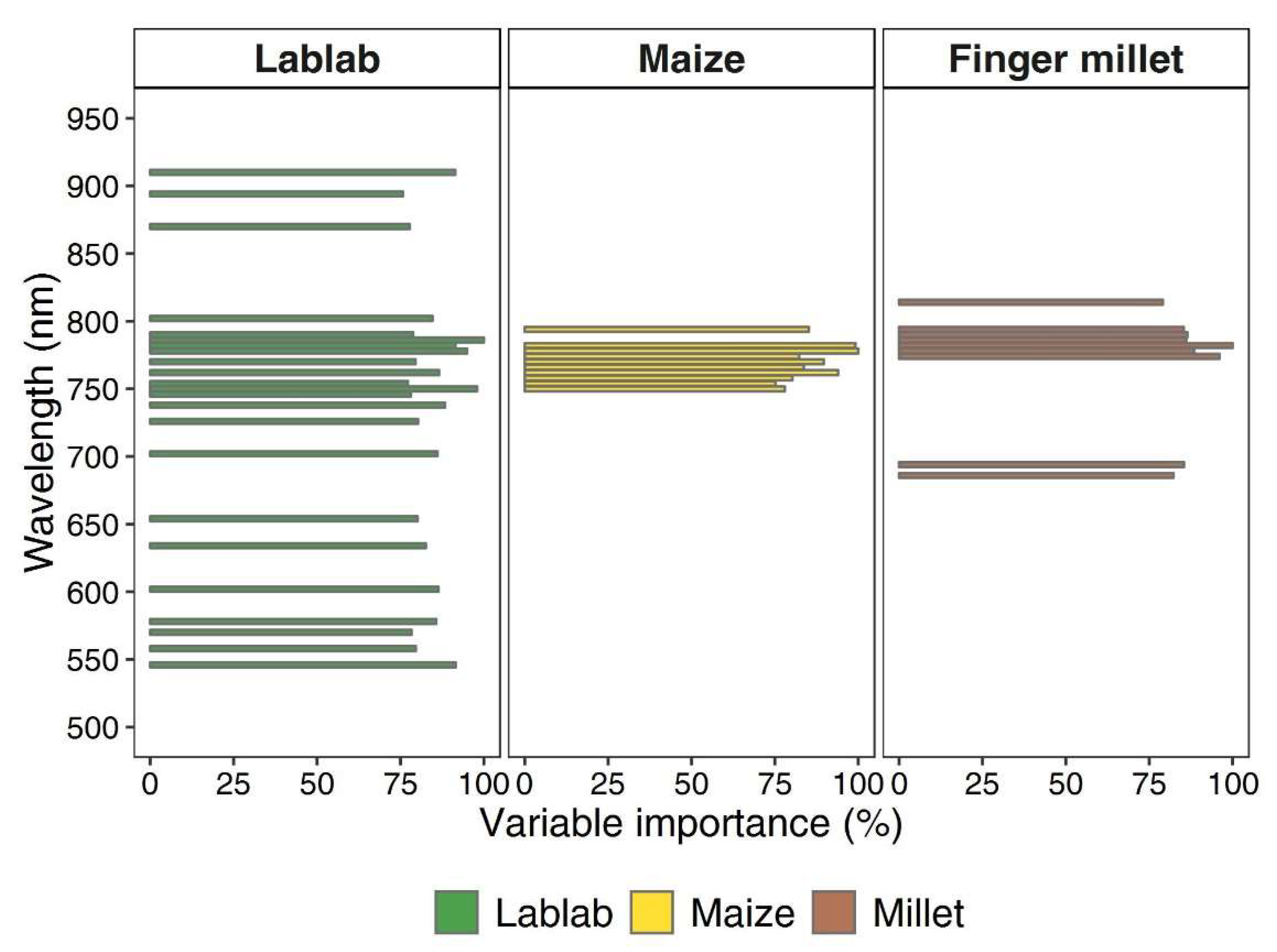
3.3. Importance of Wavelengths

The wavelengths of the crop helped in differentiating and identifying the crop traits based on their spectral region. The best model was identified out of 100 Generalised models on each crop based on the lowest RMSE value. From the best model, the wavelengths contributing above 75% in the prediction of FMB were identified, as shown in Figure 10. For lablab, it was found that a multitude of spectral bands from the green, red and near infrared (NIR) region (546–910 nm) contributed significantly to the estimation of biomass. Contrastingly, for maize, only wavelengths in the NIR region (750–794 nm) and for finger millet in both the red and NIR region (686, 694, and 774–814 nm) were important.

4. Discussion

The aim of the study was to estimate the monsoon crop biomass for three crops (lablab, maize and finger millet) based on terrestrial hyperspectral imaging during crop growth season across three years (2016–2018). With a high number of samplings during three consecutive monsoon seasons, a wide range of phenological stages of crops could be covered. This is an important issue considering the validity range of prediction models, since the harvest time of crops varies considerably in agricultural practice, for example due to nutrient and water availability and moisture content of grains. Thus, by our deliberate multi-temporal approach, the validity range of Generalised models was significantly broadened, which was further enhanced by the integration of crop measurements under a wide range of N fertiliser and water supply.

The FMB models were developed based on the predicted FMB values and tested with the observed FMB values for validation. Overall, the results indicate that the Generalised models had higher estimation accuracy (with rRMSEP ranging from 13.9% to 18.7%) for all the three crops, as compared to the rainfed and irrigated models. One reason may be that, with the combination of data from two experiments, representing severe water limitation (Rainfed experiment) and optimum water supply (Irrigated experiment), the range of crop productivity became much broader, which eventually may have increased the robustness of regression models.

Similar prediction errors were found in a previous study for maize biomass by RGB images (relative error 16.66%, R² = 0.78) [40]. In contrast to our study, their models included canopy height parameter additional to RGB information, which shows the promising potential of structural data calculated with photogrammetric methods particularly when they are combined with data from other sensor types [11,41,42]. Although spectral information was limited to the Red Edge Modified Ratio Index (REMRI), the combination of spectral data with LiDAR-derived metrics produced only a slightly smaller error in the estimation of maize biomass [10] as compared to our study. However, as the sampling was done at only one date of one single year and because no defined N and water supply was applied, the transferability of such modelling approaches beyond the study area may be limited.

Although lablab is an important legume in the food and cattle production system in India, this plant has not been subjected to any remote sensing assessment this far. The fact that it was the least productive crop in both experiments across all years, strongly reduced the range of FMB values for model calibration. However, the highest prediction errors obtained were between those of the more productive crops maize and finger millet. Similarly, finger millet is a rarely researched crop in terms of remote sensing. In a single-year satellite-based study with pearl millet, which exhibits a similar growth pattern as finger millet, Lambert et al. [43] found a strong relationship between Sentinel-2 based LAI data and crop biomass (R² = 0.84), which is much higher than in our study (R² = 0.46). Although neither sensors and platforms, nor the range of crop phenology and management were comparable, this study highlights the scope of well-informed satellite-based hyperspectral imagery, and proximal imagery may make important contributions to such developments, e.g., by the provision of crop-specific spectral libraries as a source of reference spectra that can aid the interpretation of hyperspectral and multispectral image [44].

Although we observed quite some deviation between predicted and observed FMB, the median was close to zero at all levels of N and water supply, when the Generalised models were used for all the three crops. This proves the robustness of models, which allow biomass prediction irrespective of varying nitrogen and water management practices. However, the pronounced pattern of deviations along the sampling dates in Y1 and Y2 points at the limitations of models, which are solely built on spectral information. Although soil-containing pixels were masked out of the images prior to model calibration, a substantial overestimation of biomass at the initial sampling dates in the growing season occurred, while biomass was frequently underestimated at later sampling dates. The overestimation of biomass may be caused by weeds at the initial sampling dates as the effect of weeds could not be controlled in the estimation of biomass. Further, the prediction error for crops increased in the order lablab (13.9%), finger millet (18%) and maize (18.7%), which clearly shows that spectral information captured at the top canopy layer is increasingly less representative of the biomass at lower layers of the canopy. This effect is also addressed as the “saturation constraint” and was regularly found in previous studies (e.g., [45,46,47]) particularly when vegetation indices, such as the Normalised Differential Vegetation Index (NDVI), were used. Obviously, this problem cannot be circumvented by the use of individual spectral wavelengths instead of vegetation indices, but stresses the vital necessity to develop multi-sensor approaches, in which each sensor’s shortcomings are compensated by other sensors [10,48,49].

As a common trait for all three crops, wavelengths in the red-edge area were of utmost importance for the estimation of crop biomass. The Generalised model for lablab further comprised several wavelengths in the green, red and NIR region, indicating a larger number of variables in these models. Similar important bands were found by Manjunath et al. [50] in the discrimination of chickpea, pea and lentils. While in maize the most important variables were found in the red-edge region, the model of finger millet also contained wavelengths in the red region as important variables. For lablab, several bands were identified in the visible part of spectrum (450–750 nm) to be important for biomass prediction. These bands are known to be affected by plant pigments, especially by chlorophyll [51]. The ability of lablab to fix atmospheric nitrogen may have resulted in longer greenness of the leaves over the growing period, which leads to a higher reflectance at the green peak (~550 nm) and a higher absorbance in red (~650 nm). In general, the identified spectral bands confirm accepted knowledge about biomass-reflectance relationships [52].

5. Potential and Limitations

Although Generalised models performed better at various management practices, the application of terrestrial hyperspectral measurements is still time consuming and cannot be applied on larger scales. Contrarily, drone techniques carry great potential to collect hyperspectral imagery in a comparable spatial resolution for larger areas. Another limitation is the dependence of the relative prediction error of the models from the growth development of the crops, which may have been enhanced by the change of crop varieties across years.

6. Conclusions

It has been shown that random forest regression modelling based on multi-temporal hyperspectral imagery allows the prediction of fresh matter biomass of three major food and feed crops, i.e., lablab, maize and finger millet, grown in the monsoon season on vast areas of southern India. The results of this study showed that Generalised models, which were built on crop data from both rainfed and irrigated conditions, are more robust than water management specific models. For all Generalised crop models, deviations between predicted and observed values were independent of N fertiliser and water supply, indicating a wide validity range of the models. However, an overestimation of crop biomass was detected at initial growth stages of crops along with an underestimation at the later stages of the crop growth, which was particularly pronounced with the more productive crops maize and finger millet. While wavelengths in the red edge region were important variables in all three Generalised crop models, several others in the visible and near infrared region were important in models for lablab and finger millet. The results of this study suggest that, for the tested monsoon crops at advanced maturity, even hyperspectral information is not sufficient for an accurate biomass prediction. Data fusion from a combination of sensors may improve the prediction performance, as complementary sensors can compensate for their respective deficiencies. Although lablab and finger millet are important food and cattle crops in South India, there is surprisingly little research done up to date, thus further research in this field will be of major importance considering the dynamic changes in societal and climatic conditions in this region.

References

1. Arjun, K.M. Indian Agriculture-Status, Importance and Role in Indian Economy. Int. J. Agric. Food Sci. Technol. 2013, 4, 343–346. [Google Scholar]
2. Ferrant, S.; Selles, A.; Le Page, M.; Herrault, P.A.; Pelletier, C.; Al-Bitar, A.; Mermoz, S.; Gascoin, S.; Bouvet, A.; Saqalli, M.; et al. Detection of irrigated crops from Sentinel-1 and Sentinel-2 data to estimate seasonal groundwater use in South India. Remote Sens. 2017, 9, 1119. [Google Scholar] [CrossRef]
3. Thenkabail, P.; Dheeravath, V.; Biradar, C.; Gangalakunta, O.R.P.; Noojipady, P.; Gurappa, C.; Velpuri, M.; Gumma, M.; Li, Y. Irrigated area maps and statistics of India using remote sensing and national statistics. Remote Sens. 2009, 1, 50–67. [Google Scholar] [CrossRef]
4. Cohen, Y.; Alchanatis, V.; Zusman, Y.; Dar, Z.; Bonfil, D.J.; Karnieli, A.; Zilberman, A.; Moulin, A.; Ostrovsky, V.; Levi, A.; et al. Leaf nitrogen estimation in potato based on spectral data and on simulated bands of the VENμS satellite. Precis. Agric. 2010, 11, 520–537. [Google Scholar] [CrossRef]
5. Samborski, S.M.; Tremblay, N.; Fallon, E. Strategies to make use of plant sensors-based diagnostic information for nitrogen recommendations. Agron. J. 2009, 101, 800–816. [Google Scholar] [CrossRef]
6. Zhang, F.; Zhou, G. Estimation of vegetation water content using hyperspectral vegetation indices: A comparison of crop water indicators in response to water stress treatments for summer maize. BMC Ecol. 2019, 19, 18. [Google Scholar] [CrossRef] [PubMed]
7. Aasen, H.; Burkart, A.; Bolten, A.; Bareth, G. Generating 3D hyperspectral information with lightweight UAV snapshot cameras for vegetation monitoring: From camera calibration to quality assurance. ISPRS J. Photogramm. Remote Sens. 2015, 108, 245–259. [Google Scholar] [CrossRef]
8. Rouse, J.W.; Haas, R.H.; Schell, J.A.; Deering, D.W. Monitoring vegetation systems in the great plains with ERTS. NASA Spec. Publ. 1974, 1, 309–317. [Google Scholar]
9. Warren, G.; Metternicht, G. Agricultural applications of high-resolution digital multispectral imagery: Evaluating within-field spatial variability of Canola (Brassica napus) in Western Australia. Photogramm. Eng. Remote Sens. 2005, 71, 595–602. [Google Scholar] [CrossRef]
10. Wang, C.; Nie, S.; Xi, X.; Luo, S.; Sun, X. Estimating the biomass of maize with hyperspectral and LiDAR data. Remote Sens. 2017, 9, 11. [Google Scholar] [CrossRef]
11. Moeckel, T.; Dayananda, S.; Nidamanuri, R.; Nautiyal, S.; Hanumaiah, N.; Buerkert, A.; Wachendorf, M. Estimation of vegetable crop parameter by multi-temporal UAV-borne images. Remote Sens. 2018, 10, 805. [Google Scholar] [CrossRef]
12. Burkart, A.; Aasen, H.; Alonso, L.; Menz, G.; Bareth, G.; Rascher, U. Angular dependency of hyperspectral measurements over wheat characterized by a novel UAV based goniometer. Remote Sens. 2015, 7, 725–746. [Google Scholar] [CrossRef]
13. Yu, K.; Li, F.; Gnyp, M.L.; Miao, Y.; Bareth, G.; Chen, X. Remotely detecting canopy nitrogen concentration and uptake of paddy rice in the Northeast China Plain. ISPRS J. Photogramm. Remote Sens. 2013, 78, 102–115. [Google Scholar] [CrossRef]
14. Vigneau, N.; Ecarnot, M.; Rabatel, G.; Roumet, P. Potential of field hyperspectral imaging as a non destructive method to assess leaf nitrogen content in wheat. F. Crop. Res. 2011, 122, 25–31. [Google Scholar] [CrossRef]
15. Yue, J.; Feng, H.; Jin, X.; Yuan, H.; Li, Z.; Zhou, C.; Yang, G.; Tian, Q. A comparison of crop parameters estimation using images from UAV-mounted snapshot hyperspectral sensor and high-definition digital camera. Remote Sens. 2018, 10, 1138. [Google Scholar] [CrossRef]
16. Krishna, G.; Sahoo, R.N.; Singh, P.; Bajpai, V.; Patra, H.; Kumar, S.; Dandapani, R.; Gupta, V.K.; Viswanathan, C.; Ahmad, T.; et al. Comparison of various modelling approaches for water deficit stress monitoring in rice crop through hyperspectral remote sensing. Agric. Water Manag. 2019, 213, 231–244. [Google Scholar] [CrossRef]
17. Koppe, W.; Gnyp, M.L.; Hennig, S.D.; Li, F.; Miao, Y.; Chen, X.; Jia, L.; Bareth, G. Multi-temporal hyperspectral and radar remote sensing for estimating winter wheat biomass in the North China Plain. Photogramm. Fernerkundung Geoinf. 2012, 3, 281–298. [Google Scholar] [CrossRef]
18. Knight, J.F.; Lunetta, R.S.; Ediriwickrema, J.; Khorram, S. Regional scale land cover characterization using MODIS-NDVI 250 m multi-temporal imagery: A phenology-based approach. GIScience Remote Sens. 2006, 43, 1–23. [Google Scholar] [CrossRef]
19. Aasen, H.; Gnyp, M.L.; Miao, Y.; Bareth, G. Automated Hyperspectral Vegetation Index Retrieval from Multiple Correlation Matrices with HyperCor. Photogramm. Eng. Remote Sens. 2014, 80, 785–795. [Google Scholar] [CrossRef]
20. Honkavaara, E.; Saari, H.; Kaivosoja, J.; Pölönen, I.; Hakala, T.; Litkey, P.; Mäkynen, J.; Pesonen, L. Processing and assessment of spectrometric, stereoscopic imagery collected using a lightweight UAV spectral camera for precision agriculture. Remote Sens. 2013, 5, 5006–5039. [Google Scholar] [CrossRef]
21. Yue, J.; Yang, G.; Li, C.; Li, Z.; Wang, Y.; Feng, H.; Xu, B. Estimation of winter wheat above-ground biomass using unmanned aerial vehicle-based snapshot hyperspectral sensor and crop height improved models. Remote Sens. 2017, 9, 708. [Google Scholar] [CrossRef]
22. Byre Gowda, M. DOLICHOS BEAN—Lablab Purpureus (L.) Sweet. Available online: http://www.lablablab.org/html/general-information.html (accessed on 15 May 2019).
23. Selected State-Wise Area, Production and Productivity of Ragi in India (2016-17). Available online: https://www.indiastat.com/table/agriculture-data/2/ragi-finger-millet/17200/1131134/data.aspx (accessed on 16 May 2019).
24. Prasad, J.V.N.S.; Rao, C.S.; Srinivas, K.; Jyothi, C.N.; Venkateswarlu, B.; Ramachandrappa, B.K.; Dhanapal, G.N.; Ravichandra, K.; Mishra, P.K. Effect of ten years of reduced tillage and recycling of organic matter on crop yields, soil organic carbon and its fractions in alfisols of semi arid tropics of Southern India. Soil Tillage Res. 2016, 156, 131–139. [Google Scholar] [CrossRef]
25. University of Agricultural Sciences Bangalore Agrometeorology. Available online: https://www.uasbangalore.edu.in/index.php/research/agromoterology (accessed on 21 July 2019).
26. Byre Gowda, M. HA-4, a new variety of Lablab purpureus introduced for cultivation in Karnataka. In Proceedings of the Annual Plant Breeder’s Conference, Bangalore, India, 23–25 October 2007. [Google Scholar]
27. Byre Gowda, M. Genetic Enhancement of Dolichos Bean through Integration of Conventional Breeding & Molecular Approaches and Farmers Participatory Plant Breeding. 2011. Available online: https://www.kirkhousetrust.org/docs/reports/dolichos_report_april_2011.pdf (accessed on 22 June 2019).
28. Hybrid mai.ze vari.etal desc.Ription. Available online: http://e-krishiuasb.karnataka.gov.in/ItemDetails.aspx?depID=1&subDepID=1&cropID=4# (accessed on 14 June 2019).
29. Kaul, J.; Dass, S.; Manivannan, A.; Singode, A.; Sekhar, J.C.; Chikkappa, G.K.; Parkash, O. Maize hybrid and composite varieties released in India. Tech. Bull. 2010, 80. [Google Scholar]
30. Project Coordinating Unit Compendium of Released Varieties in Small Millets. 2014. Available online: https://www.dhan.org/smallmillets/docs/report/Compendium_of_Released_Varieties_in_Small_millets.pdf (accessed on 22 June 2019).
31. Hyperspectral Imaging—Real Snapshot Technology—Cubert GmbH. Available online: https://cubert-gmbh.com/ (accessed on 3 April 2019).
32. SphereOptics Zenith LiteTM Ultralight Targets. Available online: http://sphereoptics.de/en/product/zenith-lite-ultralight-targets/ (accessed on 22 July 2019).
33. Cao, F.; Yang, Z.; Ren, J.; Jiang, M.; Ling, W.-K. Does normalization methods play a role for hyperspectral image classification? arXiv 2017, arXiv:1710.02939. [Google Scholar]
34. Zadoks, J.C.; Chang, T.T.; Konzak, C.F. A decimal code for the growth stages of cereals. Weed Res. 1974, 14, 415–421. [Google Scholar] [CrossRef]
35. Max, K.; Wing, J.; Weston, S.; Williams, A.; Keefer, C.; Engelhardt, A.; Cooper, T.; Mayer, Z.; Kenkel, B.; The R Core Team; et al. Caret: Classification and Regression Training 2018. Available online: https://cran.r-project.org/web/packages/caret/index.html (accessed on 22 June 2019).
36. Breiman, L. Random forests. Mach. Learn. 2001, 45, 5–32. [Google Scholar] [CrossRef]
37. Ismail, R.; Mutanga, O.; Kumar, L. Modeling the potential distribution of pine forests susceptible to Sirex Noctilio infestations in Mpumalanga, South Africa. Trans. GIS 2010, 14, 709–726. [Google Scholar] [CrossRef]
38. Raschka, S. Model evaluation, model selection, and algorithm selection in machine learning. arXiv 2018, arXiv:1811.12808. [Google Scholar]
39. Kvalseth, T.O. Cautionary note about R2. Am. Stat. 1985, 39, 279–285. [Google Scholar]
40. Li, W.; Niu, Z.; Chen, H.; Li, D.; Wu, M.; Zhao, W. Remote estimation of canopy height and aboveground biomass of maize using high-resolution stereo images from a low-cost unmanned aerial vehicle system. Ecol. Indic. 2016, 67, 637–648. [Google Scholar] [CrossRef]
41. Bendig, J.; Bolten, A.; Bennertz, S.; Broscheit, J.; Eichfuss, S.; Bareth, G. Estimating biomass of barley using Crop Surface Models (CSMs) derived from UAV-based RGB imaging. Remote Sens. 2014, 6, 10395–10412. [Google Scholar] [CrossRef]
42. Cunliffe, A.M.; Brazier, R.E.; Anderson, K. Ultra-fine grain landscape-scale quantification of dryland vegetation structure with drone-acquired structure-from-motion photogrammetry. Remote Sens. Environ. 2016, 183, 129–143. [Google Scholar] [CrossRef] [Green Version]
43. Lambert, M.J.; Blaes, X.; Traore, P.S.; Defourny, P. Estimate yield at parcel level from S2 time serie in Sub-Saharan smallholder farming systems. In Proceedings of the 2017 9th International Workshop, Analysis of Multitemporal Remote Sensing Images (MultiTemp), Brugge, Belgium, 14 November 2017. [Google Scholar]
44. Rama Rao, N.; Garg, P.K.; Ghosh, S.K. Development of an agricultural crops spectral library and classification of crops at cultivar level using hyperspectral data. Precis. Agric. 2007, 8, 173–185. [Google Scholar]
45. Pimstein, A.; Karnieli, A.; Bonfil, D.J. Wheat and maize monitoring based on ground spectral measurements and multivariate data analysis. J. Appl. Remote Sens. 2007, 1, 013530. [Google Scholar]
46. Freeman, K.W.; Girma, K.; Arnall, D.B.; Mullen, R.W.; Martin, K.L.; Teal, R.K.; Raun, W.R. By-plant prediction of corn forage biomass and nitrogen uptake at various growth stages using remote sensing and plant height. Agron. J. 2007, 99, 530–536. [Google Scholar] [CrossRef]
47. Baez-Gonzalez, A.D.; Chen, P.; Tiscareno-Lopez, M.; Raghavan, S. Using satellite and field data with crop growth modeling to monitor and estimate corn yield in Mexico. Crop Sci. 2002, 42, 1943–1949. [Google Scholar] [CrossRef]
48. Reddersen, B.; Fricke, T.; Wachendorf, M. A multi-sensor approach for predicting biomass of extensively managed grassland. Comput. Electron. Agric. 2014, 109, 247–260. [Google Scholar] [CrossRef]
49. Kross, A.; McNairn, H.; Lapen, D.; Sunohara, M.; Champagne, C. Assessment of RapidEye vegetation indices for estimation of leaf area index and biomass in corn and soybean crops. Int. J. Appl. Earth Obs. Geoinf. 2015, 34, 235–248. [Google Scholar] [CrossRef] [Green Version]
50. Manjunath, K.R.; Ray, S.S.; Panigrahy, S. Discrimination of spectrally-close crops using ground-based hyperspectral data. J. Indian Soc. Remote Sens. 2011, 39, 599–602. [Google Scholar] [CrossRef]
51. Kokaly, R.F.; Asner, G.P.; Ollinger, S.V.; Martin, M.E.; Wessman, C.A. Characterizing canopy biochemistry from imaging spectroscopy and its application to ecosystem studies. Remote Sens. Environ. 2009, 113, S78–S91. [Google Scholar] [CrossRef]
52. Ollinger, S.V. Sources of variability in canopy reflectance and the convergent properties of plants. New Phytol. 2011, 189, 375–394. [Google Scholar] [CrossRef] [PubMed]
Figure 1. (a) Location of Bengaluru within India; (b) design of rainfed experimental layout; (c) design of irrigated experimental layout (adjusted from [11]).
Remotesensing 11 01771 g001
Figure 2. Workflow showing the data collection (green), data preparation (yellow) and data analysis (blue).
Remotesensing 11 01771 g002
Figure 3. Fresh matter biomass (FMB) in the rainfed (R) and irrigated (I) experiment for 2016–2018 (Y1–Y3). The diagrams show average values over three levels of N fertiliser application.
Remotesensing 11 01771 g003
Figure 4. Minimum, average and maximum spectral reflectance curves of lablab, maize and finger millet for three levels of N and two levels of water supply during the three monsoon seasons.
Remotesensing 11 01771 g004
Figure 5. Prediction accuracy measured as R²val (a) and rRMSEP (b) values of the models (Rainfed, Irrigated and Generalised) for fresh matter biomass of lablab, maize and finger millet. Models were built on data from three different years, three levels of N and two levels of water supply (i.e., rainfed and irrigated).
Remotesensing 11 01771 g005
Figure 6. Plot of fit of the Generalised models for fresh matter biomass (FMB) of lablab, maize and finger millet. Each plot shows predictions from 100 RFR models with randomly selected calibration and validation data. Models were built on data from three different years, three levels of N and two levels of water supply (i.e., rainfed and irrigated).
Remotesensing 11 01771 g006
Figure 7. Normalised deviation between predicted and measured biomass for lablab, maize, and finger millet at three levels of N application (low, medium and high). Predictions were based on the Generalised model. Values were averaged over 11 sampling dates (2016–2018) and two levels of water supply (i.e., rainfed and irrigated).
Remotesensing 11 01771 g007
Figure 8. Normalised deviation between predicted and measured fresh matter biomass (FMB) for lablab, maize and finger millet at each sampling date (S1–S5) over three years (Y1–Y3). Predictions were based on the Generalised model. Values were averaged over 11 sampling dates (2016–2018) and two levels of water supply (i.e., rainfed and irrigated).
Remotesensing 11 01771 g008
Figure 9. Normalised deviation between predicted and measured biomass for lablab, maize and finger millet at two levels of water supply (rainfed and irrigated). Predictions were based on the Generalised model. Values were averaged over 11 sampling dates (2016–2018) and two levels of water supply (i.e., rainfed and irrigated).
Remotesensing 11 01771 g009
Figure 10. Important wavelengths (score above 75) in the Generalised models for fresh matter biomass of lablab, maize and finger millet. Models were built on data from three different years, three levels of N and two levels of water supply (i.e., rainfed and irrigated).
Remotesensing 11 01771 g010