Abstract
The observation error covariance (R) matrix is a key component in the data assimilation (DA) process for retrieval of atmospheric state parameters (ASPs), also impacting the subsequent numerical weather forecast. However, one commonly used type of R matrix depends on instrument noise, which contravenes reality because the retrieved ASPs would depend on the instrument used. Other types of R matrix rely on the observation operator (H), analyzed state (), background error covariance (B) matrix or the background state (), and the selected forecast ensemble. All these dependences reduce the representativeness of the R matrix, since the correctness of H needs verification and no true values exist for or . As such, a better method to correctly specify the R matrix is needed. Through the physical mechanism occurring between incident radiation and particles in the atmosphere, which complies with the phenomena of energy absorption and emission, correlations among bands or channels in a detected atmospheric radiance spectrum occur. This paper thus proposes a data-derived R matrix based on a large number (N) of detected atmospheric radiance spectra constructed from N real-time measurements, where N real-time measurements can be acquired by staring at some observation location of interest during a short amount of time. This data-derived R matrix for satellite radiance observations does not rely on any assumed quantities and is unambiguous. Technically, recording N real-time measurements is achievable by modifying the trigger configuration of data recording from ground.
1. Introduction
Modern numerical weather prediction (NWP) systems require accurate determination of the initial atmospheric state to produce a reliable weather forecast. This is achieved through data assimilation (DA). The DA attempts to blend two sources of information, the observations and the background fields, which are weighted by their respective error statistics. Although many types of observations can be assimilated in NWP systems, we focused on satellite observations, which have been found to have the largest impact of all the different observation types [1]. The observation error covariance matrix (R matrix) describes the deviation of observed radiances from true (or expected) radiances, and the background error covariance matrix (B matrix) describes the difference between the background state and the true atmospheric state. Ideally, R and B matrices should be independent of each other. Unfortunately, the design of most current DA systems forces the two to interact with each other to some extent (i.e., through iterative optimization) [2]. As a result, analysis based on the DA process highly depends on R and B matrices. However, the R and B matrices are not perfectly known, contributing to the uncertainty of subsequent weather forecasts.
While forecast is affected by analysis, it is also affected by the forecast model. This paper focuses on DA, and has little to do with forecast. Beside and matrices, the analysis also depends on the DA methodology. For global NWPs, DA methods started as simple horizontal interpolation methods [3]. Later, more advanced approaches were developed, such as three-dimensional (3D) or four-dimensional (4D) with a multivariate relationship [4]. For example, 3D and 4D variational methods were created to minimize the cost function to determine the optimal analyzed state based on a priori state, observations, and the prescribed Gaussian uncertainty statistics for the background and observations [5]; various forms of ensemble Kalman filters were introduced to consider the flow-dependent forecast (i.e., background) error covariance in the DA process [6], since background errors are expected to be flow-dependent on weather conditions. Later, hybrid approaches combining variational and ensemble DA methods were proposed [7,8], where an ensemble was used to build the initial background error covariances followed by evolving or updating the background error covariances by the NWP forecast model at the end of the DA process. Hybrid DA methods have become more popular and been employed at several NWP centers and groups [9,10,11,12,13,14,15,16,17,18,19,20,21,22]. More information on the formulation of various DA methods can be found in Gustafsson et al. [23] and Bannister [24].
The DA methods are processed under some assumptions when minimizing the cost function. In practical applications, however, these assumptions are difficult to justify [25]. One assumption that plays a critical role in DA process is about the B matrix (see review by Bannister [24] and references therein). If variational DA methods are used in operations, the B matrix is assumed to be static for a set period of time [26]. If ensemble-variational DA methods are employed in operations, the B matrix is assumed to be flow-dependent and to evolve with NWP forecast during the time window. In general, the B matrix is estimated from forecast ensemble. However, it is not clear how much the variation within the forecast ensemble can represent the background deviation from the true atmospheric state. The NWP model engaged for evolution of B matrix in the ensemble-variational DA process contains uncertainty or model error. As such, the derived B matrix is likely not representative.
Another assumption that plays an important role in DA process is about the R matrix. Until recently, the diagonal R matrix has been engaged in most operational DA systems at NWP centers [27]. Therein, instrument noise (plus forward model uncertainty and representativeness error) is placed in ’s diagonals by leaving zeros in ’s off-diagonals. However, from a physical viewpoint and as shown by many studies, inclusion of inter-channel error correlations in the R matrix is physically sound and may improve analysis accuracy [28,29,30,31,32,33,34,35,36,37,38]. Other studies have focused on diagnosing inter-channel error correlations in assimilation analysis for certain observation [39,40,41,42,43,44,45,46]. Currently the Met Office has already accounted for inter-channel error correlations in operational global and regional systems for Atmospheric Infrared Sounder (AIRS), Infrared Atmospheric Sounding Interferometer (IASI), and Cross-track Infrared Sounder (CrIS) instruments [23]. Note that the term “inter-channel error correlations” in this paper refers to correlations among channels or bands of a detected radiance spectrum in which each radiance channel or band corresponds to its specified physical quantity, such as temperature, water vapor, gas compositions, surface temperature, and emissivity, in the atmosphere.
Since 1963, many methods have been developed for quantifying the inter-channel error correlations in the R matrix [47,48,49,50,51,52]. Among these methods, the one proposed by Desroziers et al. [52] has been widely used to estimate the observation error variances and inter-channel error correlations in Météo-France [52] and ECMWF (European Center for Medium-Range Weather Forecasts) [37] 4D-Var systems, and has also been applied to IASI data to estimate the structure of R matrix in the Met Office 4D-Var system [39]. Desroziers et al.’s scheme [52] was combined with the maximum-likelihood approach to estimate the spatial correlation length-scale of observation errors [53]. Some other studies also applied this technique [35,39,52], for example.
As the R matrix based on Desroziers et al. [52] relies on the observation operator (H), analyzed state (), B matrix or background state (), and selected forecast ensemble, all of which contain uncertainties, the R matrix used in the DA process may cause some problems. For example, the convergence speed of the DA process may decrease [27,39], which might indicate a possible limitation of those inter-channel error correlations and problems in the methods used to estimate the R matrix in DA process [2]. The most common problem is that this R matrix is not symmetrical (note that symmetry is a necessity for R matrix), leading to the eigenvalues of this R matrix being not positive-definite (note that positive-definite eigenvalues are required in DA process). Thus, this R matrix must be artificially made to be symmetrical and the eigenvalues must be altered to be positive-definite prior to their use in assimilation systems [2,35,39]. Tabeart et al. [2] suggested that these problems are caused by the interaction between the R and B matrices. The interaction is a numerical interaction rather than a physical interaction, which is a well-known issue during the iterations of the DA process in an effort to produce optimal outcomes for succeeding weather forecasts.
Given the above limitations, a better method to characterize R matrix is needed, as stated in previous studies [2,23,39]. Since the assumptions used in estimating R and B matrices are not always valid, reduction or entire elimination of the dependency on the assumptions and complete separation of the R matrix from the B matrix should enable us to produce a more physically sound R matrix. This study introduces a potential method to derive the R matrix, which requires no additional assumptions. Following the path of radiation through the atmosphere up to the radiation received by sensors and transformed to radiance, the correlations among the channels or bands in a detected atmospheric radiance spectrum allows us to propose a data-derived R matrix. This R matrix is built fully based on a large number (N) of detected atmospheric radiance spectra constructed from N real-time measurements (Appendix A), where N real-time measurements can be acquired by observing some location of interest during a short amount of time. The only two requirements in the data derivation of the R matrix are the fabrication of instruments and the data calibration procedures, which are fundamental for any data analysis.
Our first motivation for creating a data-derived R matrix using a large number of real-time measurements is as follows. In traditional approaches, the derived R matrix based on statistical forecast ensemble cannot fully represent the observation errors because it is unclear how much the variation within the ensemble sample can represent the observation errors (i.e., variance and covariance) between observed and true radiance. This derived R matrix may not fully characterize the atmospheric state of an interested moment. Conversely, since real-time measured data contain representative information of the atmospheric state at the time when the data were recorded, the derived R matrix based on real-time data can appropriately characterize the observation errors for the atmospheric state at that time when data were recorded. One critical difference between our proposed method and traditional approaches is that our proposed data-derived R matrix is built without assumptions (i.e., no dependence on , , , or matrix), whereas the traditional R matrices are constructed upon some assumptions that may not be always valid. The other motivation for this study is the desire to inspire the community to consider completely using real-time data to construct R matrix for satellite radiance observations from a different perspective.
Three notes need to be explained. Firstly, the method proposed in this paper for construction of a data-derived matrix is only applicable to satellite measurements. Secondly, the meaning of “a large number of measurements” used here does not refer to the multi-measurements that are used in current numerical weather prediction within a certain time window. For multi-measurements, one single measurement is taken from each observation location at a moment of interest and thus multi-measurements correspond to multiple different atmospheric states. We do not use multi-measurements to construct the matrix because the matrix constructed from multiple different atmospheric states may be good enough within the time period when the multi-measurements were recorded, but not necessary ideal for assimilating the measurements. Thirdly, this paper presents the theoretical basis of a data-derived matrix based on N real-time measured radiances and suggests a conceptual design of a trigger configuration for satellites to record N real-time measurements. To record N real-time measurements, practical experimentation is required.
This paper is organized as follows. Section 2 briefly describes the methods that have been used to estimate the R matrix in literature. Remarks are provided about these methods and the long-used diagonal-only R matrix. Section 3 explains (i) radiation transmission through atmosphere and the radiation received at the sensors of an instrument and transformed to radiance, and (ii) the accompanying correlations among bands or channels of a detected atmospheric radiance spectrum. These are used to form the theoretical basis of the data-derived R matrix using N real-time measured radiances. Section 4 lists the advantages of using a data-derived matrix. Since no real data currently exist for constructing a data-derived matrix, Section 5 presents a conceptual design of a trigger configuration for satellites to record such data, and Section 6 provides simple simulation data with simple toy examples to demonstrate our proposed method. Our summary and recommendations for future work are discussed in Section 7 and Section 8, respectively.
2. Estimation of the R Matrix
In this section, the existing methods for constructing the matrices are introduced. The common factor among these methods is that they are based on the use of a single measurement (Appendix A). For example, Rodgers [54] and Daley [55] described the developments in these methods, and Rogers [56] reviewed these methods in 1976. However, no single measurement is exact [57] because each measurement of atmospheric state must have varying degrees of error.
By focusing on some observation location of interest, one potential solution is to record a large number of real-time measurements during a short amount of time (Appendix A). These data can be used to derive the R matrix without any assumption, and the derived R matrix is completely free from dependence on H, , and (or B matrix). This is the focus of Section 3.
2.1. Earlier Methods
Among methods for quantifying inter-channel error correlations, the simplest method [47,48] uses a least square fit of an isotropic correlation model to the correlation sample, which is statistically collected from observation-minus-background (OMB) among all pairs of stations. By extrapolating the obtained fit curve to the origin, the ratio between the observation and background (i.e., forecast) error standard deviation can be determined. The extracted error covariance parameters are approximately homogeneous and isotropic and vary slowly with season.
Hollingsworth and Lönnberg [49] analyzed the statistical structure of errors from OMB and partitioned the errors into background and observation error components, which is called the Hollingsworth and Lönnberg method. The background here means the calculated radiance from H(). This method was built with statistical ensemble and was established based on two assumptions: Firstly, the background and observation errors are independent of each other, and, secondly, the background errors are homogeneously correlated in the horizontal plane while the observation errors are horizontally uncorrelated.
Due to the assumptions made in Hollingsworth and Lönnberg method, Dee and Da Silva [50] raised questions about this method’s robustness and argued that background errors and observation errors could be correlated with each other. Dee and Da Silva [50] thus proposed a method to evaluate the background error and observation error covariance parameters based on maximum-likelihood covariance parameter estimation as described in Dee [58]. This method produced statistical error covariance parameters that varied with time. However, the assumption of correlations between background and observation error covariance parameters results in interaction or trade-offs between background error and observation error covariance parameters during iterations of the DA process, and ultimately, the acquired error covariance parameters may deviate from the true content. This is the fundamental limitation of this method if multiple parameters are entangled during simultaneous estimation.
Inspired by the generalized cross-validation approach [59,60], Desroziers and Ivanov [51] proposed a method to tune the observation error and background error covariance parameters based on observation-minus-analysis (OMA) from statistics of analysis innovations. The tuning was achieved using a randomization technique with a perturbation of either observations or background fields when computing the statistical average of the cost function’s values at minima.
A method based on the combinations of OMB, OMA, and background-minus-analysis (BMA) for statistical estimation of the background errors (for the B matrix), observation errors (for the R matrix), and analysis errors was proposed by Desroziers et al. [52]. This method has become the most popular for estimation of the observation errors (i.e., variance and covariance) in the R matrix. The next section presents the formation of the R matrix based on this method.
2.2. Desroziers’ R Matrix
Below, we only focus on the construction of the R matrix. Desroziers et al. [52] and Stewart et al. [35] provide more details. Denote as the background innovation vector, which is the difference between the observations , and their background counterparts H(), where the superscript o denotes observation. Similarly, is the analysis innovation, which is the difference between the observations and their analysis counterparts, H(). Upon the first assumption of no correlation between background and observation errors, Desroziers et al. [52] showed that the statistical expectation of the product of and approximates the R matrix. According to Desroziers et al. [52], the covariance of innovation is ; the covariance of and is . Therefore, the latter covariance representing R matrix is presented in Equation (1).
where the superscript D denotes the method by Desroziers et al., indices i and j are the band or channel numbers of a radiance spectrum, and index k runs over all forecast ensemble from 1 to N. The second assumption made by Desroziers et al. is that H, , and B matrix are accurate when the matrix constructed using Equation (1) is applied in analyses. Unfortunately, uncertainties always exist in H, , and B matrix. As a consequence, problems arise.
The first fundamental problem is that this matrix is not uniformly symmetrical [30,35,50]. Since is not necessarily equal to for component i, and is not necessarily equal to for component j:
which is a result of the violation of the second assumption introduced by Desroziers et al. This is also a violation of the physical requisite for data analysis. The issue caused by the asymmetric matrix is that the eigenvalues of this matrix are not all positive (i.e., not positive definite). Therefore, prior to using this matrix in assimilation systems, artificial treatments are required to symmetrize the asymmetrical matrix (by taking the mean of the original matrix and its transpose matrix) and to modify any negative eigenvalue to be positive [39]. Some other treatments, as proposed in Desroziers et al., involve applying an iterative procedure for updating the contents of matrix until matrix is closer to being symmetrical [35,52]. Regardless of which treatment is employed, the resulting matrix is influenced by the specification of H, , and B matrix, which are not perfectly known.
The second fundamental problem is experienced by all methods proposed in literature, which is the use of statistical forecast ensemble in the derivation of the R matrix [47,48,49,50,51,52] as well as of the B matrix. Strictly, the variation among the forecast ensemble may not fully reflect the departure of real observations from the true atmospheric state at that time when data were recorded, and thus the extent to which this derived R matrix can represent the true observation error covariance matrix for the atmospheric state at that time when data were recorded cannot be ascertained.
2.3. Diagonal-Only R Matrix
The diagonal-only observation error matrix ( matrix), where instrument noise plus forward model uncertainty and representativeness error are placed in ’s diagonals by leaving zeros in ’s off-diagonals, is still used in many atmospheric research analyses and operational weather forecast (ARWF). For this case, the observation error in ’s diagonals is given by [39,56]:
where is the observation error between the observed radiance and the true radiance . Hence, the diagonal matrix is:
with being the transpose of . According to previous studies [39,56], is interpreted as instrument noise (plus forward model uncertainty and representativeness error).
The first remark on this diagonal matrix is that the retrieved atmospheric state parameters (ASPs; referring to temperature, water vapor, gas compositions, surface temperature, emissivity, etc.) rely on which instrument is being used because the instrument noise is included in the matrix. This contravenes reality because real ASPs are independent of any instrument and thus retrieved ASPs should be independent of any instrument. Given a measured system (e.g., an atmospheric state), suppose that we use M different instruments to measure the same atmospheric state, each of which instrument has a different level of noise. Regardless of the instrument used, any known level of instrument noise needs to be subtracted and not included in the data analysis so that the output of the analysis is not be affected by the instrument used. Rather than observation noise (or named error or variation) induced by measurements within a measured system, note that here we are discussing instrument noise due to the instrument itself that generally can be obtained from laboratory experiments.
In terms of measurements, the observed radiance at a given time is one of many varying radiances around the true radiance . Thus, the second remark is that in Equation (3) should be interpreted as a pure deviation between the observed and the true rather than instrument noise. Unfortunately, since single measurement (Appendix A) has been used in ARWF, neither the true nor this variance is obtainable. The observed and true vary with scenes (i.e., atmospheric states); thus, the observation errors in an R matrix vary with atmospheric states. So, pre-launch measurements from the laboratory are unable to provide information about variances for an R matrix. It is crucial that this variance is not equal to instrument noise in general. Recent studies [35,39] have demonstrated that diagonal elements in an observation error covariance matrix have visible differences from instrument noise. Therefore, use of the diagonal-only matrix imposes some limitations in analyses.
3. Data-Derived R Matrix
Physically, correlations exist among bands or channels of a detected atmospheric radiance spectrum. This section explains these correlations based on the phenomena of energy absorption and emission caused by electron transition, which have been observed in the study of electromagnetic radiation absorbed and emitted by atoms [61] and have been applied in the study of radiative properties occurred in atmosphere [62]. This is followed by the derivation of an R matrix using N detected radiance spectra constructed from N real-time measurements acquired by observing some location of interest for a short amount of time.
3.1. Physical Mechanism of Radiation Through Atmosphere
An atmospheric state in thermodynamic equilibrium (hereafter, “atmospheric state in equilibrium”) is viewed from macroscopic aspects, whereas any fluctuation state (around equilibrium) caused by physical processes between radiation and atmosphere is viewed from microscopic aspects. One fluctuation state is acquired from one single measurement, and a macroscopic equilibrium is composed of many microscopic fluctuation states, among which fluctuation states are almost or exactly balanced. Therefore, given an observation location over a short amount of detection time, the atmospheric state in equilibrium may not be reflected by any single measurement, but by the average of a large number of measurements.
Figure 1 depicts the radiation spectrum and which parts of that spectrum are detected by the instrument sensor. The region between two adjacent black lines in the radiation spectrum (called a segment radiation) corresponds to the measurement between the two black lines in the instrument sensor. In the following, when a radiation of a given wavenumber (or energy) is termed, this means the named segment radiation as denoted above; when a radiation without any specified wavenumber (or energy) is termed, this indicates the radiation covering all possible wavenumbers (or energies) within. Below, we present the interactions between radiation and atmosphere from microscopic aspects.
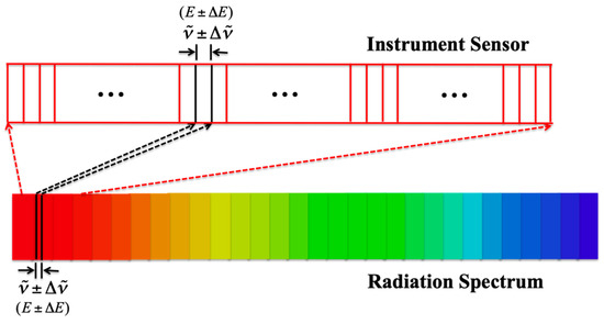
Figure 1.
Detection of a portion of radiation (e.g., infrared; lower part) by an instrument sensor (upper part), where () represents the width of wavenumber (energy) of a segment radiation (see the segment bordered by two black lines in the radiation spectrum) that is detected by the channel or band of () in an instrument sensor (see the channel or band bordered by two black lines in the instrument sensor).
When the sun’s radiation enters the earth’s atmosphere (“atmosphere” hereafter), part of the sun’s radiation in visible (VIS) and the near infrared (NIR) spectrum is reflected back to space by the atmosphere and clouds before reaching the earth’s surface. However, part of the sun’s radiation passes through the atmosphere and subsequently is reflected by the earth’s surface back to space or absorbed by the earth’s surface; simultaneously, emissions from radiation of longer wavelengths, such as infrared, are radiated out back to space from the earth’s surface and atmosphere. All these occurrences depend on the atmospheric states.
After, when radiation travels upward through the atmosphere, interactions occur between radiation and molecules and particles in the atmosphere, caused by particle targets such as , ozone, aerosol, water vapor, precipitation, and cloud [61,62]. These interaction processes include absorption, emission, elastic scattering, and inelastic scattering. Generally, the interaction processes of absorption, emission, and inelastic scattering involve energy exchange between incident radiation and particles in the atmosphere. In quantum mechanics, given the energy (E) of radiation (or photons; i.e., a segment radiation), the Planck’s energy-frequency relation states that E is proportional to its frequency (): , where h is the Planck constant, is the speed of light, and and are wavelength and wavenumber, respectively. When energy changes, its corresponding frequency (wavelength and wavenumber as well) changes as well. As a consequence, given an incident radiation of a specified energy E (or specified wavenumber ), radiation of different energy (i.e., different wavenumber ) may be emitted after the interaction. In this case, a couple of basic formations for the energy of outgoing radiation are possible. Firstly, the energy of the incident radiation can be completely absorbed by particles in the atmosphere, and no radiation is emitted as a result. Secondly, when particle targets in the atmosphere are thin, incident radiation may only lose some portion of its energy, and radiation with less energy is emitted. Thirdly, one special formation can occur. Sometimes, the particles in atmosphere absorb part or all of the energy of the incident radiation and store such energy (denoted ) inside the particles. Then, the next time another new incident radiation of energy interacts with such particles, the incident radiation may release some energy (denoted ) to the particles, but gain the energy freed from the particles. The resulting energy of the outgoing radiation, , can be greater or less than the original incident energy , depending on the positive or negative balance of .
Physically, the mechanism for the energy exchange between incident radiation and particles in the atmosphere follows the phenomena of energy absorption and emission that occur between incident radiation and atoms (or molecules) [61]. Therefore, the wavenumber (or energy) of the outgoing radiation can be zero (i.e., no outgoing radiation), less, or greater than that of the incident radiation. This means that with respect to the wavenumber () of the incident radiation, the wavenumber () of the outgoing radiation can be different from that of the incident radiation and range from zero to infinity, though we know an infinite wavenumber is impossible. This suggests that radiation of wavenumber is correlated with the radiation of wavenumber .
The same physical mechanism is applied to all segments in a radiation beam. After radiation beams pass through the atmosphere, the detected radiation at the sensors installed on an instrument is transformed to radiance in terms of per steradian per square meter during a short detection time frame, forming an atmospheric radiance. Recall the meaning of inter-channel error correlations among bands or channels provided in Section 1. The statement “radiation of wavenumber has correlations to radiation of wavenumber ” equivalently suggests that a channel or band of wavenumber has physical correlations with the channel or band of wavenumber in a detected atmospheric radiance spectrum. From microscopic aspects, the notion of atmospheric fluctuation states induced by various extents of interactions between radiations and particles in the atmosphere allow us to examine correlations among those atmospheric physical variables (e.g., temperature, water vapor, various gas compositions, surface temperature, emissivity, etc.) via studying correlations among the channels or bands of a detected atmospheric radiance spectrum. The extent of the correlations depends on the atmospheric state at the time when data are recorded. All these can be explored through the observation error covariance (R) matrix that is presented in the next section using a large number of real-time measurements of radiance spectra.
3.2. Construction of Data-Derived R Matrix
Before proceeding, some notes about the differences among instrument noise, instrument random error, and observation error are provided. Instrument noise (as noise equivalent delta temperature) is produced by the instrument itself, independent of measurements of a measured system (e.g., atmospheric state here), and is usually obtainable from the laboratory. Instrument random error, produced by instrument itself as well, may occur during measurements and is usually uncontrollable and random. Observation error, independent of the instrument, is caused by atmospheric variations. Recall the macroscopic versus microscopic aspects mentioned earlier. Each atmospheric variation state corresponds to one fluctuation state (viewed from a microscopic aspect). An atmospheric state in equilibrium (viewed from macroscopic aspects) can be determined from averaging many atmospheric variation (or fluctuation) states.
Construction of an R matrix directly based on statistical measured data has been commonly used in many experiments, such as fundamental sciences in physics and chemistry. Here, we introduce this approach to the construction of an matrix in atmospheric sciences. By observing some location of interest within a solid view angle during a short amount of detection time around a limited area , suppose that N measurements of radiance spectra (Appendix A) are collected with a given instrument. The N measured radiance spectra are used to construct one R matrix for this observation location of interest. Each measurement contains spectral radiance bands or channels. Denote indices i and j as band or channel numbers and index k runs from 1 to N measurements. For the kth measurement, the measured radiance (i) for the ith band or channel can be expressed as:
where is the true value of radiance and is induced by atmospheric variation (and instrument random error, if any). The variation in each radiance band or channel is assumed to be a Gaussian or Gaussian-like distribution, which is widely accepted in real world practices. Any known instrument noise and any known non-signal events (if any) are subtracted in Equation (5) since they are irrelevant to the physical quantity that describes the measured system. Note that physical quantity and measured system can be referred to as atmospheric state parameters and atmospheric state, respectively, in our case.
From N measured radiance spectra:
where is the mean value of measured radiance for the ith band or channel, is the uncertainty of , and is the variance of . Given the band or channel i, the N measurements of can be equivalently regarded as a single measurement of N-dimensional vectors. Each band or channel, hence, has its own mean value and associated uncertainty that are obtained from the N-dimensional vectors. For a radiance spectrum of bands or channels, the joint probability density function (p.d.f) is the product of Gaussians [63,64]:
where , , and are abbreviations of , , and , respectively. The vector quantity is the true value of vector (i.e., the radiance spectrum describing an atmospheric state in equilibrium) and is given as a function of vector and vector , , where denotes known parameters (such as atmospheric pressures) and vector represents unknown parameters (such as atmospheric state parameters of an atmospheric state in equilibrium). The least square method is used to extract the quantity . Here, the physical meaning of is the same as the observation operator accordingly, is replaced by hereafter.
Taking the logarithm of the joint p.d.f. and dropping those terms unrelated to the vector gives the log-likelihood function:
The quantity can be found by minimizing the quantity:
Equations (8) and (9) are used to describe the situation among which bands or channels of a radiance spectrum are independent. However, due to the effects of correlations among bands or channels, the term should be replaced by a covariance matrix R, and Equations (8) and (9) accordingly become:
where . Modified from the variance in Equation (6), the covariance between the ith and jth bands or channels is expressed as:
and should be placed in R’s off-diagonal elements. This data-derived matrix is guaranteed to be symmetrical, which meets the DA process requirement. Moreover, the correlation, between the ith and jth bands or channels is then given by:
Using standard error propagation, the covariance matrix for estimated is given by:
where means the found that is closest to the true . The diagonals in are the variances of the corresponding variances of vector .
Equations (6)–(14) are well known and can be found in textbooks of probability theory and statistics or related [63,64]. The reason why we introduce them here is to remind people that the R matrix used in the DA system of ARWF can be obtained directly from a large number of real-time measured radiance spectra, rather than using diagonal-only or constructing matrix based on theoretical H, human-assumed B matrix, and , which cause problems in the DA process as mentioned previously.
Then, how does the data-derived R matrix work on the cost function? The role of the in Equation (11) is the same as the second term (inside the braces) in the cost function used in the current DA system:
except that is either or , and single measurement at each observation location is used in . Conversely, we propose using the average from N measurements recorded at each observation location for the cost function in the DA system:
where is given in Equation (12). The notation m runs over all included observation locations from various instruments during a certain time window.
4. Advantages of Using Data-Derived R Matrix
There are many advantages of using data-derived matrix, such as independence on forward model, , or for , no forward model uncertainty, no representative error, no entanglement with matrix, and symmetric matrix etc. Several other advantages are explained below.
1. View from Macroscopic and Microscopic Aspects
An atmospheric state in equilibrium can be viewed from a macroscopic viewpoint that is composed of many microscopic aspects, where each microscopic aspect represents one fluctuation state around the macroscopic state in equilibrium. That is, by taking repeated measurements at an observation location during a short amount of time, each measurement represents one fluctuation state, whereas the average of those repeated measurements is regarded as the expectation of the truth of the macroscopic state in equilibrium. The deviation between each measurement and the average is the observation error and is used for constructing a data-derived matrix.
2. Accurate Expectation of True Radiance
The matrix in Equation (1) is constructed based on Desroziers et al. [52], where and are taken as the true radiance . However, and are the radiance calculated from a radiative transfer model or algorithm (i.e., forward model) upon assumptions such that relies on , , and (or matrix).
For a data-derived matrix, in probability and statistics theory [63,64], the expected value (known as expectation) of a variable is the average value of repeated measurements of the same experiments. Taking the average of repeated measurements as the expectation of the true value of a variable is generally used in experimental measurements [57]. We here apply such a concept to the data-derived matrix by taking the average of the observed radiance (i.e., , see Equation (6)) as the expectation of the true radiance , which is consistent with what is stated in note 1).
3. Correlations Accounted Among All Physical Quantities
The data-derived matrix does not only address one particular atmospheric physical quantity, but also contains information of variances and correlations for all atmospheric physical quantities, where each radiance band or channel corresponds to its own representative atmospheric physical quantity. simply characterizes the variance of atmospheric physical quantity in the ith radiance band or channel, and the correlation between any two atmospheric physical quantities in the ith and jth bands or channels can be readily obtained by Equation (13).
4. Less Flow Dependency
The observation error in an observation error covariance matrix is defined as the difference between the observed radiance and the true radiance , and attained and depends on the weather conditions at the time when data are recorded. The messages in the data-derived matrix thus only depend on the weather conditions at a given observation location at a given time. Therefore, given an observation location at a time of interest, the data-derived built in Equation (12) is only computed once. Hence, there is no need to update the data-derived matrix within a DA process period. This considerably reduces computation time as compared with the traditional approach. The current DA system and the proposed DA system are compared in Figure 2.
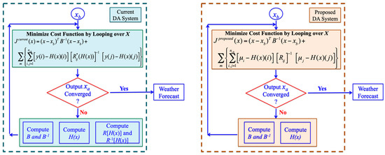
Figure 2.
(a) Current data assimilation (DA) system (left) versus (b) proposed DA system (right), where the DA systems are indicated inside dashed squares. Note that can be either or in the current DA system.
In the current DA system (Figure 2a), if the output from the DA process is not converged, adjustments to both (i.e., either or ) and matrices are needed before processing the next DA cycle. This leads to complexity in the DA process and a less accurate used for next-step weather forecast because the greater the number of factors (i.e., and matrices here) influencing , the greater the uncertainty associated with . Conversely, in the proposed DA system (Figure 2b), at each given observation location and time, the content in the data-derived matrix is only calculated once and fixed during iterations of the DA process. Thus, only the matrix needs adjustment for next cycle of the DA process if has not converged. This approach simplifies the DA process as compared with the traditional approach and is expected to produce a more accurate because only one factor (i.e., the matrix) needs adjustment in the DA process. Note that must be computed in each iteration of both DA systems.
5. Temporal Variations of Inter-Channel Error Correlations
In the current DA system, the or matrix is usually assumed to be static for the day, a few days, or even for months. The messages in an observation error covariance matrix depend on weather conditions. Therefore, the data-derived matrix allows us to quantify the change in inter-channel error correlations over time, where the change in the magnitude of ’s messages relies on how quickly the weather conditions change over time. Currently, there are no such real-time data; thus, we are unable to present the magnitude of change in this paper.
6. Gaussian Distribution of Variation
Here provides a supplementary explanation to the cost functions. The expression in both Equations (15) and (16) is basically derived from the least square method [63,65] upon the assumption of Gaussian or Gaussian-like distribution of variation in each radiance band or channel [63], which is widely accepted in real world practices as mentioned previously. This means that the variation in each radiance band or channel follows a Gaussian or Gaussian-like distribution. A large enough sample can be used to verify if the distribution is a Gaussian or Gaussian-like distribution. However, recording only a few measurements does not prevent the variation in each radiance band or channel from behaving as a Gaussian or Gaussian-like distribution if the variation does follow a Gaussian or Gaussian-like distribution.
5. Conceptual Design of Proposed Trigger Configuration
Technically, taking a large number of measurements within a short detection time (Appendix A) is achievable by modifying the trigger configuration of data recording from ground, based on a private communication with specialists in hyper-spectral hardware instruments. As for the number of measurements within needed, this may require simulation and/or practical experimentation by considering the desired extent of uncertainty in the analyses. This uncertainty includes that induced by atmospheric variation and instrument systematic variation, and the uncertainty level, which can be obtained by the covariance matrix in Equation (14), would be revealed in the retrieved atmospheric state parameters.
The traditional trigger configuration continuously takes single measurements, with each measurement taken within detection time (Appendix A), where not all data are yet used in practice. To fully use the collected data, the trigger configuration is proposed to take N measurements within with some time separation () between two consecutive N measurements, regardless of the low earth orbit (LEO) detection sources or geosynchronous satellites. Figure 3 illustrates the traditional trigger configuration (TTC) versus the proposed trigger configuration (PTC). The load of the data recorded with the PTC can thus be reduced and would be less expensive.
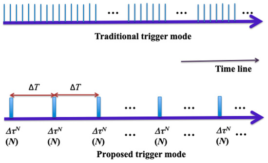
Figure 3.
Traditional trigger configuration (TTC) versus proposed trigger configuration (PTC), where each blue bar represents detection time when scanning one location. Symbol denotes taking N measurements within .
The detection time may be longer than . Both and can be studied using simulation and/or practical experimentation. The fluctuation in the measured radiance, possibly due to recording a large number of measurements within a short time span, does not have any significant impact on the retrieved ASPs (see the study presented in Section 6.1). Therefore, if we use data recorded with the TTC in the future, the long-term issues and costs due to inaccurate weather forecasts that we have experienced at least since the first satellite was launched for taking atmospheric data would continue, which would outweigh the cost of data captured with PTC.
6. Simple Simulation Studies
Since no such real data exist, we instead used simulation data with simple toy examples to demonstrate how the data-derived matrix works and how the retrieved outputs perform compared with the methods employed in current DA systems. This was inspired by Desroziers et al. [52], where simulation data with toy examples were used to demonstrate their methods. Figure 4 illustrates the simple simulation example, where three bands or channels were considered for simplification. The atmospheric state parameters are represented as and the measured radiance at the instrument sensor is described as . The relationship between and is through matrix , which is . The first term in the cost function, , was unable to be simulated in this study and thus is ignored here, which would not affect the purpose of our demonstration. Four different observation operators were adopted in this study as follows:
and
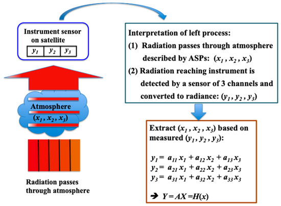
Figure 4.
Simple toy examples employed to demonstrate the performance of the data-derived matrix.
In the following, notations corr, cr, and wr denote correlation, correct, and wrong, respectively; () means and/or are/is used rather than indicating that is a function of . Hence, () is taken as a correct (), both and (both and ) are taken as two incorrect ’s (two incorrect ’s), and both and (both and ) are used for illustration of correlations between any two channels or bands. is assigned as the true values of ASPs in the equilibrium state; radiances and are regarded as representing two fluctuation states around an atmospheric state in equilibrium and are obtained according to when single measurement is considered, where is a Gaussian distribution centered at zero with a deviation of 0.05 if no other deviation values are applied elsewhere; and is the averaged radiance from N measured radiances. Similar to what is usually performed in DA analysis, when looking for the best that is closest to , is restricted within during minimization of the cost function. Note that equation used for radiance generation and for construction of matrix is abbreviated as hereafter. For a large number of measurements, N = 200 is used in our study.
Below, we present four cases (Cases A–D). The purpose of Case A (Section 6.1) was to demonstrate the importance of verification for correctness of H and to investigate the impact of fluctuation in measured radiances on the retrieved . The questions addressed in Case B (Section 6.2) were: Is diagonal-only matrix appropriate? Is single measurement enough? Does need verification? Similar to Case B, the purpose of Case C (Section 6.3) was to answer: Is matrix appropriate? Is single measurement enough? Does need verification? Finally, the purpose of Case D (Section 6.4) was to determine if correlations could be automatically manifested from the matrix. For each case, we described its analysis and provided results and discussions.
6.1. Case A
Firstly, N sets of measured radiances were obtained from N real-time measurements, which were generated according to . The data-derived matrix was then constructed using the N sets of radiances based on Equations (6) and (12). Subsequently, the second term of the cost function in Equation (16) was minimized by looping over to look for the best using various (). Lastly, the uncertainty of each retrieved in could be obtained from the covariance U matrix (Equation (14)).
The fluctuation in measured radiance could be magnified as a result of taking N measurements over a short time span. To visualize the effect of taking N measurements on the retrieved , the fluctuation was simulated by the deviation in the Gaussian function. Deviation values of 0.05, 0.10, 0.15, 0.20, 0.30, and 0.40 were investigated, and the corresponding generated radiances were denoted by or simply hereafter, with subscript d representing the deviation values. The procedure of this analysis is depicted in Figure 5.
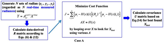
Figure 5.
Analysis procedures for Cases A.
The results are listed in Table 1. In the cost function (Figure 5), is the average of all N sets of measured radiances, considered as the expectation of true radiance; and the matrix was fully built from real-time data, providing good representativeness of the true matrix. As seen in Table 1, only a correct () could produce a correct that was consistent with the true , where both the cost function value and the uncertainty for each retrieved were the smallest. Note that the best would fall outside with a bigger value if any component of the retrieved reaches the boundary of . This suggests that verification of the correctness of (or the forward model) is necessary for ASP retrieval in a DA system.

Table 1.
Results for Case A, where or represent data from N measured radiances. The second column means the matrix is based on what for construction and the third column represents what () is used in minimization.
Under the same conditions except for deviation values, the results show that the extracted values of using various deviations (i.e., various extents of fluctuation) were almost the same. Hence, only the results using deviations of 0.05, 0.15, and 0.40 are listed in Table 1. These results indicate that fluctuation in measured radiances did not have any significant impact on the retrieved even when the deviation was up to 40%.
We noted three features in Table 1. The first one was that the bigger the deviation, the smaller the value of . This occurred because the matrix was in the denominator of the cost function and a larger fluctuation produced bigger errors and bigger error correlations in the matrix, resulting in smaller value. The second feature was that the value for the case using was smaller than when using because was chosen to be closer to than . The third feature was that the larger the deviation (i.e., fluctuation) in the measured radiances, the greater the uncertainties in the retrieved , which was reasonable.
6.2. Case B
Single measurement for radiance (or ) and diagonal-only matrix were considered in this case. Firstly, (or ) was adopted as the measured radiance with the existence of deviation from the average of radiance . Secondly, the variances in the matrix were taken from the diagonal variances of the ensemble-derived matrix, where the ensemble-derived matrix in Case B was built using N sets of ensemble radiances that were generated according to with , , or . Unlike the current DA process in which the matrix varies with when it needs re-computation during minimization iterations, was used to compute the ensemble-derived matrix for all minimization iterations in Case B (and Case C as well). The purpose for doing so was to imitate the consideration of forward model uncertainty and representativeness error in the ensemble-derived matrix and ’s diagonals so that both the ensemble-derived matrix and ’s diagonals were as close as the true matrix. Thirdly, the second term of the cost function in Equation (15) was minimized by looping over to look for the best using various (), where and (or ) were used here. Note that the () matrix used in building the ensemble-derived matrix (i.e., the second step) and minimization of the cost function (i.e., the third step) were the same. Finally, the uncertainty of each retrieved in could be obtained from the covariance U matrix. The procedure of this analysis is displayed in Figure 6.
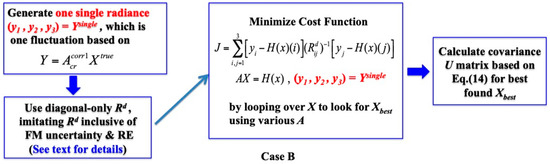
Figure 6.
Analysis procedures for Cases B, where FM uncertainty and RE stand for forward model uncertainty and representativeness error, respectively.
The results are presented in Table 2. No () was able to produce an consistent with because single measured radiance (or ) only represents one fluctuation state around an atmospheric state in equilibrium, introducing deviation from the equilibrium state, and because does not contain full contents. Notwithstanding, the use of a correct () in minimizing the cost function could produce an closest to with the smallest values and the least uncertainty for each retrieved , which again reveals the importance of verifying the correctness of . With respect to Case A, this study inspired us to think that a single measurement for the radiance spectrum may not be sufficient and may not be appropriate either.
Table 2.
Results for Case B, where (or ) means data from single measured radiance, the second column means matrix is based on what for construction, and the third column represents what () is used in minimization.
6.3. Case C
The analysis procedure in Case C was the same as that in Case B except taken from the ensemble-derived matrix was adopted. See Figure 7 for the analysis procedure.
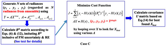
Figure 7.
Analysis procedures for Cases C, where FM uncertainty and RE stand for forward model uncertainty and representativeness error, respectively.
The results are shown in Table 3. Another study was conducted using for all constructions, the results of which are provided in Table 4. No () was able to produce an consistent with . Similar to Case B, this occurred because (or ) was used and might not possess good representativeness of the true matrix. Once again, using a correct () to minimize the cost function could produce an closest to with the smallest values and least uncertainty for each retrieved . As such, verification of the correctness of is important.
Table 3.
Results for Case C, where (or ) denotes data from single measured radiance, the second column means the matrix is based on what for construction, and the third column represents what () is used in minimization.
Table 4.
Results for Case C, where (or ) denotes data from single measured radiance, the second column means the matrix is based on what for construction, and the third column represents what () is used in minimization.
In summary, the findings from Cases A, B, and C provided some important learnings. Firstly, with the adoption of N real-time measured radiances, constructing the data-derived matrix from N measured radiances, and the correct observation operator could produce an consistent with with the smallest value and almost the least uncertainty for each retrieved (see the first result in each case of using different deviations in Table 1). Secondly, conversely, if or together with single measured (or ) was employed, discrepancy appeared in the retrieved compared to . Thirdly, as long as a correct was used in the minimization of the cost function, the retrieved was closest to with the smallest value and the least uncertainty for each retrieved . This reveals the importance of verifying the correctness of (or the forward model) used in the DA process. One important result was that fluctuation in the measured radiances did not have any significant impact on the retrieved , even when the deviation was up to 40%. This suggests that fluctuation possibly caused by taking N measurements (if any) is not an issue.
Although linear was employed in our toy simulation studies, the conclusions presented here should be the same even if the real was non-linear. That is because the nonlinear forward problem could be linearized around the background.
6.4. Case D
The generation of the data-derived matrix in Case D was the same as that in Case A, where () and () were employed for illustration of correlations between any two channels or bands. Once the data-derived matrix was built, the correlation matrix was acquired based on Equation (13). Figure 8 outlines the analysis procedure.
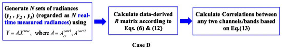
Figure 8.
Analysis procedures for Cases D.
The results of the correlations are listed in Table 5. When using (), the off-diagonals in the data-derived matrix were much smaller than those in the diagonals, resulting in much smaller correlations in the off-diagonals than those in the diagonals. Conversely, if () was used, the magnitudes in the diagonals and off-diagonals in the data-derived matrix were comparable, and the correlations in both the diagonals and off-diagonals were also comparable. This study demonstrates that the correlations between any two channels or bands could be manifested from the matrix itself. Therefore, despite significant or insignificant correlations between any two channels or bands, the data-derived matrix proposed in this paper provides a method to acquire correlations between any two channels or bands (i.e., correlations between any two atmospheric physical quantities).
Table 5.
Results for Case D, where or indicate data from N measured radiances, and the second column means the matrix was based on what for construction.
7. Summary
Atmospheric state parameter profiles (atmospheric profiles) are key inputs for numerical weather prediction. The observation error covariance (R) matrix factor plays a pivotal role in the retrievals of atmospheric profiles. Since a single measurement is used in atmospheric research analyses and operational weather forecast (ARWF), correct variance and covariance cannot be obtained for the R matrix. As a consequence, the diagonal matrix arranged with instrument noise (plus forward model uncertainty and representativeness error) in the diagonal elements to serve as variances by leaving zeros in off-diagonal has been used in ARWF for years. Recently, a new matrix structure based on the method of Desroziers et al. [52] was introduced and has been adopted in, for example Météo-France and ECMWF 4D-Var systems, and has also been applied to AIRS, IASI, and CrIS data in Met Office 4D-Var systems.
However, the instrument noise acting as variance in ’s diagonal led to the dependence of the retrieved ASPs on the instrument being employed. This conflicts with reality in that ASPs should not depend on any instrument. The matrix relies on H, , and the B matrix or , yet the correctness of H requires validation and no true value exists for or . This leads to the matrix being not uniformly symmetrical, resulting in eigenvalues not fully positive-definite, causing less representativeness because ’s structure depends on users’ assignment to and , users’ choices of H, and the selected forecast ensemble that generally cannot describe the atmospheric state at the time when data were captured. Even after diagnosis of the matrix through iterations in the DA process, the diagnosed matrix still has problems as reported in the literature. The problems are caused by the use of single measurement, resulting in an R matrix entangled with B matrix in the DA process.
To unentangle the R and B matrices, the complete isolation of the R matrix from the B matrix is required. To acquire correct variances and covariances for the R matrix, a potential solution is to use a large number (N) of real-time measurements within a short detection time to replace single measurement. An atmospheric state in equilibrium (viewed from macroscopic aspects) can be determined from averaging over many atmospheric variation (or fluctuation) states (viewed from a microscopic aspect). Thus, the R matrix used in the DA system for retrieval of parameters of an atmospheric state in equilibrium can be achieved by taking many fluctuation states. From a physical viewpoint based on microscopic aspects, each fluctuation state involves interactions between radiation and the particles in the atmosphere, and the interactions comply with the phenomenon of the energy absorption and emission occurring between incident radiation and atoms (or molecules). The wavenumber (i.e., energy) of the outgoing radiation may change after passing through all the layers in the atmosphere, subsequently being received at sensors installed in instruments and converted to radiance to form a radiance spectrum. This suggests correlations exist among bands or channels of a detected atmospheric radiance spectrum. Following probability theory and statistics, a correct R matrix can thus be derived based on N real-time measurements, independent of any assumed quantities, and hence having no ambiguity.
Apart from constructing the R matrix, using N real-time measurements has several other advantages. Unlike single measurement, which is merely a variation around an equilibrium state, the mean of the N measurements can adequately represent the equilibrium state during the detection time . Another advantage is that an N real-time measured sample is capable of describing the atmospheric state at the time when the data were captured, whereas forecast ensemble is generally incapable of doing so. A further advantage is that the uncertainty of the N measured radiance spectra conveys some messages. Firstly, finer structures of H would not signify if they were smaller than the uncertainty, equivalently meaning that a more precise H does not mean more accurate retrieval. Secondly, this uncertainty provides us with some information about the uncertainty level that can be tolerated on H when H is linearized, whereas linearization of H may potentially be used to verify the correctness of H using the N measured radiance spectra.
Technically, taking N measurements during a short amount of detection duration is achievable by modifying the trigger configuration of data recording from ground. The traditional trigger configuration captures single measurements successively, but many data are not used in practice. Therefore, to fully use detected data and to reduce the load of the captured data, the proposed trigger configuration involves recording N measurements within with some time between two consecutive N-measurement events. Our study revealed that fluctuation in the measured radiances that could be inferred by taking N measurements does not have any significant impact on the retrieved ASPs.
Several advantages of taking N real-time measurements of radiances for constructing a data-derived matrix were discussed in this paper. Studies using simulation data with simple toy examples were also presented in this paper. These studies demonstrate that the adoption of N real-time measured radiances, a data-derived matrix constructed from the N measured radiances, and a correct can produce accurate ASPs with smallest cost function value and the least uncertainty for each retrieved ASP. These studies also revealed that verification for correctness of (or forward model) is necessary.
8. Recommendations for Future Work
As mentioned in Section 1, the retrieval results of ASPs from the DA system for successive weather forecast depend on H, the design of the DA methods, and the information in R and B matrices. In traditional ARWF, entanglement occurs in the DA system among (1) H, which needs verification; (2) DA methods; (3) the R matrix, which relies on instrument noise or H, , and ; and (4) the B matrix whose evolution depends on the NWP (or forecast) model. Furthermore, R and/or B matrices are usually constructed from forecast ensemble rather than real-time data. Thus, even if the R matrix is acquired correctly, the DA system still cannot guarantee producing accurate retrieved ASPs without proper H, correct B, and an appropriate DA method. Therefore, to ensure the whole DA system functions properly for correct production of retrieved ASPs and for next-step weather forecasting, it is a step-by-step course. The first and easiest step would be to fully isolate the R matrix from H, , and (or B matrix) and to independently and directly acquire the R matrix from N real-time measurements as explained in this paper. After that, the following tasks would be verification of H and building the B matrix with the measured N real-time data, with the aim of being free from reliance on the NWP (or forecast) model or historical forecast ensemble. Once R, H, and B are attained without entanglement with one another, the goal would be the determination of the DA method that performs the best.
Lastly, we hope to inspire people to think from a new perspective about which one, single measurement or a large number of measurements, should be used for the matrix as well as ARWF, and what can be accomplished with a large number of measurements to improve the accuracy of the retrieval of atmospheric state parameters and of numerical weather prediction.
Author Contributions
Conceptualization, Y.-A.L., Z.L., and M.H.; Investigation, M.H.; Methodology, Y.-A.L., Z.L., and M.H.; Formal analysis, M.H.; Writing–original draft preparation, M.H.; Writing–review & editing, Y.-A.L., Z.L., and M.H.; Funding acquisition, Y.-A.L.
Funding
This work was supported by the National Natural Science Foundation of China (Grant No. 41601469).
Acknowledgments
Since 2013, M.H. has been investigating the issues in atmospheric research and weather forecast. M.H. is grateful to the Space Science and Engineering Center (SSEC) at the University of Wisconsin-Madison (Madison, WI, USA) for providing a good working environment. M.H. is indebted to SSEC’s financial support during 2016–2017 for this work. Furthermore, we would like to express our gratitude to the four reviewers for reviewing our manuscript so carefully and providing constructive comments and suggestions. We are also thankful to the academic editor for handling our manuscript and going over our manuscript and responses to the reviewers.
Conflicts of Interest
The authors declare no conflict of interest.
Appendix A. Nomenclature
- Single measurement refers to the acquisition of one single measurement inside a view angle within a short amount of detection time around a limited area by staring at some observation location of interest. Here, one single measurement means to obtain one radiance spectrum, which is adopted for retrieval of atmospheric state parameter profiles. If an interferometer is used, one single measurement indicates the acquisition of one single interferogram used to attain one radiance spectrum.
- A large number of measurements refer to collecting N (e.g., N 200) measurements inside the same within a short amount of detection time around the same by staring at some observation location of interest, where each measurement is used to construct one radiance spectrum, and the average of the N radiance spectra along with the variance and covariance is employed for retrieval of atmospheric state parameter profiles.
The superscripts S on and N on represent single measurement and N measurements, respectively. The detection time may be longer than or could be about the same, which could be studied by using real data.
References
- Thépaut, J.-N. Satellite Data Assimilation in Numerical Weather Prediction: An Overview. Available online: https://www.ecmwf.int/en/elibrary/12657-satellite-data-assimilation-numerical-weather-prediction-overview (accessed on 8 September 2003).
- Tabeart, J.M.; Dance, S.L.; Haben, S.A.; Lawless, A.S.; Nichols, N.K.; Waller, J.A. The conditioning of least-squares problems in variational data assimilation. Numer. Linear Algebr. Appl. 2018, 25, e2165. [Google Scholar] [CrossRef]
- Eliassen, A. Provisional Report on Calculation of Spatial Covariance and Autocorrelation of the Pressure Field; Report No. 5; Videnskaps-Akademiets Institutt for Vaer-Og Klimaforskning: Oslo, Norway, 1954; 12p. [Google Scholar]
- Lorenc, A.C. A Global Three-Dimensional Multivariate Statistical Interpolation Scheme. Mon. Weather Rev. 1981, 109, 701–721. [Google Scholar] [CrossRef]
- Le Dimet, F.X.; Talagrand, O. Variational algorithms for analysis and assimilation of meteorological observations: theoretical aspects. Tellus A 1986, 38A, 97–110. [Google Scholar] [CrossRef]
- Evensen, G. Sequential data assimilation with a nonlinear quasi-geostrophic model using Monte Carlo methods to forecast error statistics. J. Geophys. Res. 1994, 99, 10143–10162. [Google Scholar] [CrossRef]
- Liu, C.; Xiao, Q.; Wang, B. An Ensemble-Based Four-Dimensional Variational Data Assimilation Scheme. Part I: Technical Formulation and Preliminary Test. Mon. Weather Rev. 2008, 136, 3363–3373. [Google Scholar] [CrossRef]
- Lorenc, A.C. The potential of the ensemble Kalman filter for NWP—A comparison with 4D-Var. Q. J. R. Meteorol. Soc. 2003, 129, 3183–3203. [Google Scholar] [CrossRef]
- Buehner, M.; McTaggart-Cowan, R.; Beaulne, A.; Charette, C.; Garand, L.; Heilliette, S.; Lapalme, E.; Laroche, S.; Macpherson, S.R.; Morneau, J.; et al. Implementation of Deterministic Weather Forecasting Systems Based on Ensemble–Variational Data Assimilation at Environment Canada. Part I: The Global System. Mon. Weather Rev. 2015, 143, 2532–2559. [Google Scholar] [CrossRef]
- Gustafsson, N.; Bojarova, J. Four-dimensional ensemble variational (4D-En-Var) data assimilation for the HIgh Resolution Limited Area Model (HIRLAM). Nonlinear Process. Geophys. 2014, 21, 745–762. [Google Scholar] [CrossRef]
- Wang, X. Incorporating Ensemble Covariance in the Gridpoint Statistical Interpolation Variational Minimization: A Mathematical Framework. Mon. Weather Rev. 2010, 138, 2990–2995. [Google Scholar] [CrossRef]
- Schwartz, C.S.; Liu, Z.; Lin, H.-C.; Cetola, J.D. Assimilating aerosol observations with a “hybrid” variational-ensemble data assimilation system. J. Geophys. Res. Atmos. 2014, 119, 4043–4069. [Google Scholar] [CrossRef]
- Schwartz, C.S.; Liu, Z. Convection-Permitting Forecasts Initialized with Continuously Cycling Limited-Area 3DVAR, Ensemble Kalman Filter, and “Hybrid” Variational–Ensemble Data Assimilation Systems. Mon. Weather Rev. 2014, 142, 716–738. [Google Scholar] [CrossRef]
- Zhang, M.; Zhang, F. E4DVar: Coupling an Ensemble Kalman Filter with Four-Dimensional Variational Data Assimilation in a Limited-Area Weather Prediction Model. Mon. Weather Rev. 2012, 140, 587–600. [Google Scholar] [CrossRef]
- Gustafsson, N.; Bojarova, J.; Vignes, O. A hybrid variational ensemble data assimilation for the HIgh Resolution Limited Area Model (HIRLAM). Nonlinear Process. Geophys. 2014, 21, 303–323. [Google Scholar] [CrossRef]
- Clayton, A.M.; Lorenc, A.C.; Barker, D.M. Operational implementation of a hybrid ensemble/4D-Var global data assimilation system at the Met Office. Q. J. R. Meteorol. Soc. 2013, 139, 1445–1461. [Google Scholar] [CrossRef]
- Kuhl, D.D.; Rosmond, T.E.; Bishop, C.H.; McLay, J.; Baker, N.L. Comparison of Hybrid Ensemble/4DVar and 4DVar within the NAVDAS-AR Data Assimilation Framework. Mon. Weather Rev. 2013, 141, 2740–2758. [Google Scholar] [CrossRef]
- Bishop, C.H.; Hodyss, D. Adaptive Ensemble Covariance Localization in Ensemble 4D-VAR State Estimation. Mon. Weather Rev. 2011, 139, 1241–1255. [Google Scholar] [CrossRef]
- Wang, X.; Lei, T. GSI-Based Four-Dimensional Ensemble–Variational (4DEnsVar) Data Assimilation: Formulation and Single-Resolution Experiments with Real Data for NCEP Global Forecast System. Mon. Weather Rev. 2014, 142, 3303–3325. [Google Scholar] [CrossRef]
- Kleist, D.T.; Ide, K. An OSSE-Based Evaluation of Hybrid Variational–Ensemble Data Assimilation for the NCEP GFS. Part I: System Description and 3D-Hybrid Results. Mon. Weather Rev. 2015, 143, 433–451. [Google Scholar] [CrossRef]
- Kleist, D.T.; Ide, K. An OSSE-Based Evaluation of Hybrid Variational–Ensemble Data Assimilation for the NCEP GFS. Part II: 4DEnVar and Hybrid Variants. Mon. Weather Rev. 2015, 143, 452–470. [Google Scholar] [CrossRef]
- Liu, C.; Xiao, Q.; Wang, B. An Ensemble-Based Four-Dimensional Variational Data Assimilation Scheme. Part II: Observing System Simulation Experiments with Advanced Research WRF (ARW). Mon. Weather Rev. 2009, 137, 1687–1704. [Google Scholar] [CrossRef]
- Gustafsson, N.; Janjić, T.; Schraff, C.; Leuenberger, D.; Weissmann, M.; Reich, H.; Brousseau, P.; Montmerle, T.; Wattrelot, E.; Bučánek, A.; et al. Survey of data assimilation methods for convective-scale numerical weather prediction at operational centres. Q. J. R. Meteorol. Soc. 2018, 144, 1218–1256. [Google Scholar] [CrossRef]
- Bannister, R.N. A review of operational methods of variational and ensemble-variational data assimilation. Q. J. R. Meteorol. Soc. 2017, 143, 607–633. [Google Scholar] [CrossRef]
- Liu, Y.-A.; Huang, H.-L.A.; Gao, W.; Lim, A.H.N.; Liu, C.; Shi, R. Tuning of background error statistics through sensitivity experiments and its impact on typhoon forecast. J. Appl. Remote Sens. 2015, 9, 096051. [Google Scholar] [CrossRef]
- Kleist, D.T.; Parrish, D.F.; Derber, J.C.; Treadon, R.; Wu, W.-S.; Lord, S. Introduction of the GSI into the NCEP Global Data Assimilation System. Weather Forecast. 2009, 24, 1691–1705. [Google Scholar] [CrossRef]
- Weston, P. Progress towards the implementation of correlated observation errors in 4D-Var. In Forecasting Research Technical Report 560; Met Office: Exeter, UK, 2011. [Google Scholar]
- Rabier, F.; Fourrie, N.; Chafai, D.; Prunet, P. Channel selection methods for Infrared Atmospheric Sounding Interferometer radiances. Q. J. R. Meteorol. Soc. 2002, 128, 1011–1027. [Google Scholar] [CrossRef]
- Liu, Z.-Q.; Rabier, F. The potential of high-density observations for numerical weather prediction: A study with simulated observations. Q. J. R. Meteorol. Soc. 2003, 129, 3013–3035. [Google Scholar] [CrossRef]
- Rainwater, S.; Bishop, C.H.; Campbell, W.F. The benefits of correlated observation errors for small scales. Q. J. R. Meteorol. Soc. 2015, 141, 3439–3445. [Google Scholar] [CrossRef]
- Collard, A.D. On the choice of observation errors for the assimilation of AIRS brightness temperatures: A theoretical study. In Technical Memorandum AC/90; ECMWF: Reading, UK, 2004. [Google Scholar]
- Stewart, L.M.; Dance, S.L.; Nichols, N.K. Correlated observation errors in data assimilation. Int. J. Numer. Methods Fluids 2008, 56, 1521–1527. [Google Scholar] [CrossRef]
- Stewart, L.M.; Dance, S.L.; English, S.J.; Eyre, J.R.; Nichols, N.K. Observation Error Correlations in IASI Radiance Data; Mathematical Report Series; University of Reading: Reading, UK, 2009; Available online: https://www.researchgate.net/publication/41571544_Observation_error_correlations_in_IASI_radiance_data (accessed on January 2009).
- Stewart, L.M.; Dance, S.L.; Nichols, N.K. Data assimilation with correlated observation errors: experiments with a 1-D shallow water model. Tellus A Dyn. Meteorol. Oceanogr. 2013, 65, 19546. [Google Scholar] [CrossRef]
- Stewart, L.M.; Dance, S.L.; Nichols, N.K.; Eyre, J.R.; Cameron, J. Estimating interchannel observation-error correlations for IASI radiance data in the Met Office system. Q. J. R. Meteorol. Soc. 2014, 140, 1236–1244. [Google Scholar] [CrossRef]
- Bormann, N.; Bauer, P. Estimates of spatial and interchannel observation-error characteristics for current sounder radiances for numerical weather prediction. I: Methods and application to ATOVS data. Q. J. R. Meteorol. Soc. 2010, 136, 1036–1050. [Google Scholar] [CrossRef]
- Bormann, N.; Collard, A.; Bauer, P. Estimates of spatial and interchannel observation-error characteristics for current sounder radiances for numerical weather prediction. II: Application to AIRS and IASI data. Q. J. R. Meteorol. Soc. 2010, 136, 1051–1063. [Google Scholar] [CrossRef]
- Waller, J.A.; Dance, S.L.; Lawless, A.S.; Nichols, N.K. Estimating correlated observation error statistics using an ensemble transform Kalman filter. Tellus A Dyn. Meteorol. Oceanogr. 2014, 66, 23294. [Google Scholar] [CrossRef]
- Weston, P.P.; Bell, W.; Eyre, J.R. Accounting for correlated error in the assimilation of high-resolution sounder data. Q. J. R. Meteorol. Soc. 2014, 140, 2420–2429. [Google Scholar] [CrossRef]
- Bormann, N.; Saarinen, S.; Kelly, G.; Thépaut, J.-N. The Spatial Structure of Observation Errors in Atmospheric Motion Vectors from Geostationary Satellite Data. Mon. Weather Rev. 2003, 131, 706–718. [Google Scholar] [CrossRef]
- Bormann, N.; Geer, A.J.; Bauer, P. Estimates of observation-error characteristics in clear and cloudy regions for microwave imager radiances from numerical weather prediction. Q. J. R. Meteorol. Soc. 2011, 137, 2014–2023. [Google Scholar] [CrossRef]
- Bormann, N.; Bonavita, M.; Dragani, R.; Eresmaa, R.; Matricardi, M.; McNally, A. Enhancing the impact of IASI observations through an updated observation-error covariance matrix. Q. J. R. Meteorol. Soc. 2016, 142, 1767–1780. [Google Scholar] [CrossRef]
- Campbell, W.F.; Satterfield, E.A.; Ruston, B.; Baker, N.L. Accounting for Correlated Observation Error in a Dual-Formulation 4D Variational Data Assimilation System. Mon. Weather Rev. 2017, 145, 1019–1032. [Google Scholar] [CrossRef]
- Waller, J.; Ballard, S.; Dance, S.; Kelly, G.; Nichols, N.; Simonin, D. Diagnosing Horizontal and Inter-Channel Observation Error Correlations for SEVIRI Observations Using Observation-Minus-Background and Observation-Minus-Analysis Statistics. Remote Sens. 2016, 8, 581. [Google Scholar] [CrossRef]
- Waller, J.A.; Simonin, D.; Dance, S.L.; Nichols, N.K.; Ballard, S.P. Diagnosing Observation Error Correlations for Doppler Radar Radial Winds in the Met Office UKV Model Using Observation-Minus-Background and Observation-Minus-Analysis Statistics. Mon. Weather Rev. 2016, 144, 3533–3551. [Google Scholar] [CrossRef]
- Cordoba, M.; Dance, S.L.; Kelly, G.A.; Nichols, N.K.; Waller, J.A. Diagnosing atmospheric motion vector observation errors for an operational high-resolution data assimilation system. Q. J. R. Meteorol. Soc. 2017, 143, 333–341. [Google Scholar] [CrossRef]
- Gandin, L. Objective Analysis of Meteorological Fields; Translated from the Russian. Jerusalem (Israel Program for Scientific Translations). Q. J. R. Meteorol. Soc. 1965, 92, 242p. [Google Scholar]
- Rutherford, I.D. Data Assimilation by Statistical Interpolation of Forecast Error Fields. J. Atmos. Sci. 1972, 29, 809–815. [Google Scholar] [CrossRef]
- Hollingsworth, A.; Lönnberg, P. The statistical structure of short-range forecast errors as determined from radiosonde data. Part I: The wind field. Tellus A 1986, 38A, 111–136. [Google Scholar] [CrossRef]
- Dee, D.P.; da Silva, A.M. Maximum-Likelihood Estimation of Forecast and Observation Error Covariance Parameters. Part I: Methodology. Mon. Weather Rev. 1999, 127, 1822–1834. [Google Scholar] [CrossRef]
- Desroziers, G.; Ivanov, S. Diagnosis and adaptive tuning of observation-error parameters in a variational assimilation. Q. J. R. Meteorol. Soc. 2001, 127, 1433–1452. [Google Scholar] [CrossRef]
- Desroziers, G.; Berre, L.; Chapnik, B.; Poli, P. Diagnosis of observation, background and analysis-error statistics in observation space. Q. J. R. Meteorol. Soc. 2005, 131, 3385–3396. [Google Scholar] [CrossRef]
- Ménard, R. Error covariance estimation methods based on analysis residuals: Theoretical foundation and convergence properties derived from simplified observation networks. Q. J. R. Meteorol. Soc. 2016, 142, 257–273. [Google Scholar] [CrossRef]
- Rodgers, C.D. Inverse Methods for Atmospheric Sounding: Theory and Practice; World Scientific Publishing Pte. Ltd.: Singapore, 2000; 256p. [Google Scholar]
- Daley, R. Atmospheric Data Analysis; Cambridge University Press: Cambridge, UK, 1993. [Google Scholar]
- Rodgers, C.D. Retrieval of atmospheric temperature and composition from remote measurements of thermal radiation. Rev. Geophys. 1976, 14, 609–624. [Google Scholar] [CrossRef]
- JCGM. Evaluation of Measurement Data—Guide to the Expression of Uncertainty in Measurement. Available online: https://www.bipm.org/utils/common/documents/jcgm/JCGM_100_2008_E.pdf (accessed on 26 July 2019).
- Dee, D.P. On-line Estimation of Error Covariance Parameters for Atmospheric Data Assimilation. Mon. Weather Rev. 1995, 123, 1128–1145. [Google Scholar] [CrossRef]
- Craven, P.; Wahba, G. Smoothing noisy data with spline functions: Estimating the correct degree of smoothing by the method of generalized cross-validation. Numer. Math. 1978, 31, 377–403. [Google Scholar] [CrossRef]
- Golub, G.H.; Heath, M.; Wahba, G. Generalized Cross-Validation as a Method for Choosing a Good Ridge Parameter. Technometrics 1979, 21, 215–223. [Google Scholar] [CrossRef]
- Martin, W.C.; Wiese, W.L. Atomic Spectroscopy—A Compendium of Basic Ideas, Notation, Data, and Formulas. Available online: https://www.nist.gov/pml/atomic-spectroscopy-compendium-basic-ideas-notation-data-and-formulas (accessed on 1 November 2017).
- Yang, P.; Liou, K.-N.; Bi, L.; Liu, C.; Yi, B.; Baum, B.A. On the radiative properties of ice clouds: Light scattering, remote sensing, and radiation parameterization. Adv. Atmos. Sci. 2015, 32, 32–63. [Google Scholar] [CrossRef]
- Cowan, G. Statistical Data Analysis; Oxford University Press: Oxford, UK, 1998; 212p. [Google Scholar]
- Taylor, J.R. An Introduction to Error Analysis, 2nd ed.; University Science Books: Sausalito, CA, USA, 1996; 327p. [Google Scholar]
- Bouttier, F.; Courtier, P. Data Assimilation Concepts and Methods. Available online: https://www.ecmwf.int/node/16928 (accessed on March 1999).
© 2019 by the authors. Licensee MDPI, Basel, Switzerland. This article is an open access article distributed under the terms and conditions of the Creative Commons Attribution (CC BY) license (http://creativecommons.org/licenses/by/4.0/).