Characterizing Boreal Peatland Plant Composition and Species Diversity with Hyperspectral Remote Sensing

 , , ,
, , ,  ,
, 
Abstract
1. Introduction
2. Methods
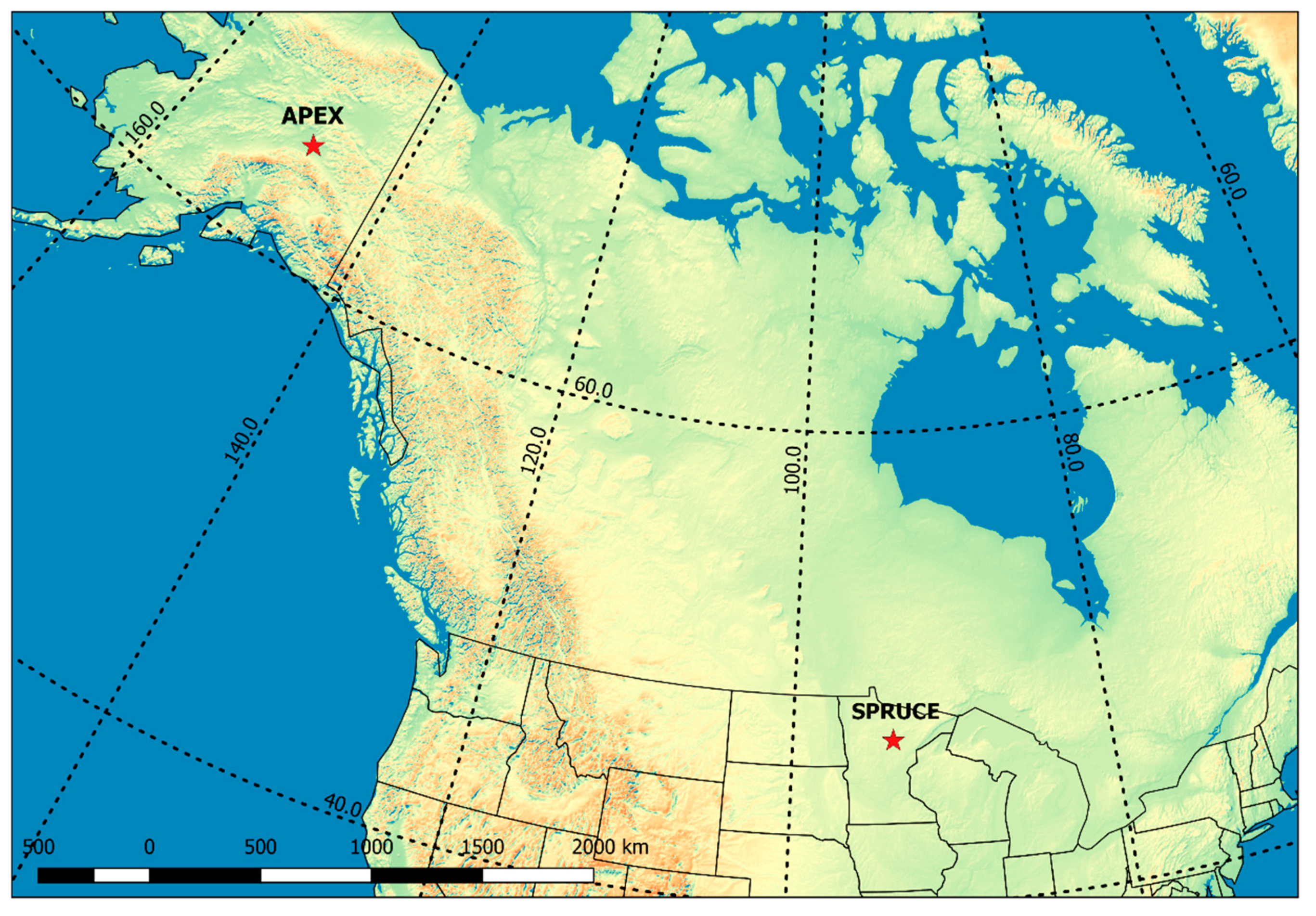
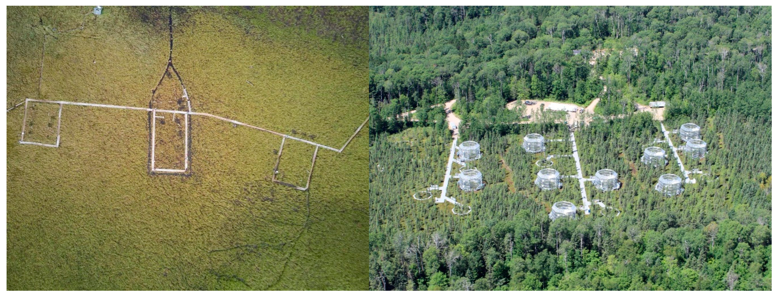
2.1. Study Sites
2.2. Data Collection
2.2.1. Vegetation Cover Sampling
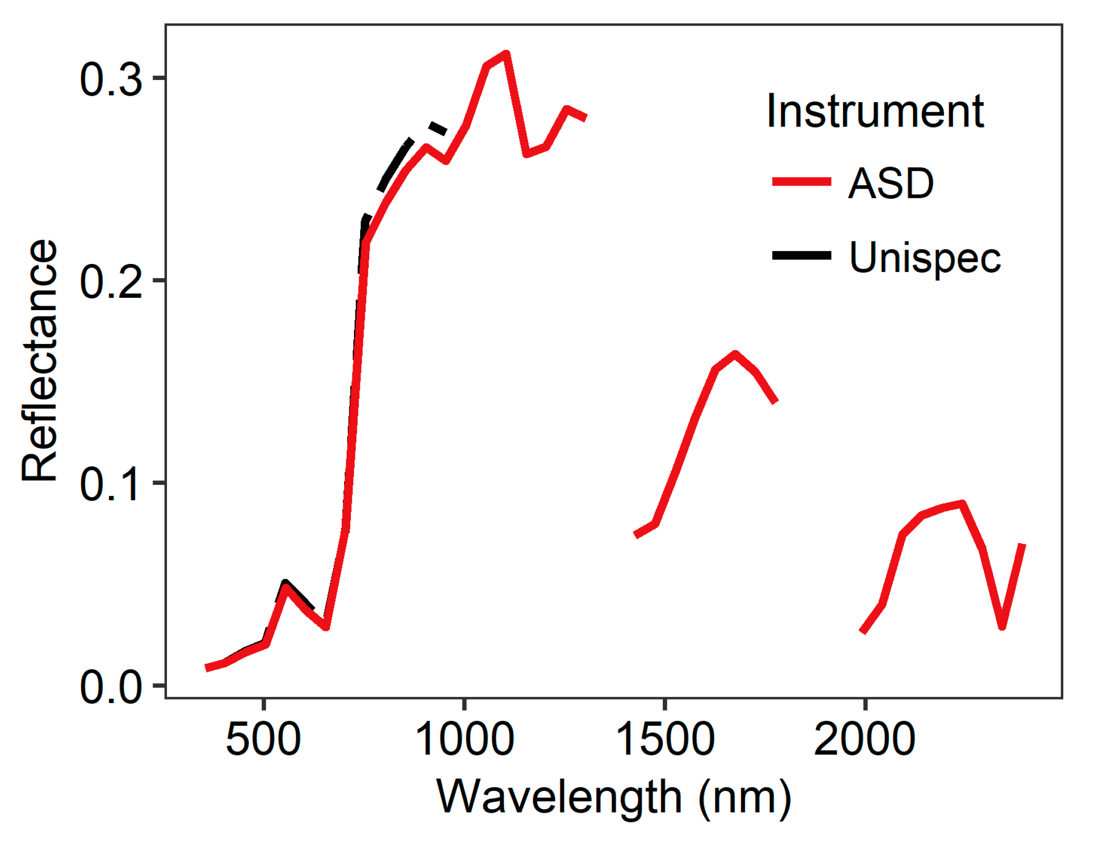
2.2.2. Spectral Sampling
2.2.3. Aerial Hyperspectral Data Collection
2.3. Data Analysis
2.3.1. Analysis of Vegetation Composition and Species Diversity
2.3.2. Spectral Data Analysis
2.3.3. Hyperspectral Image Analysis
3. Results
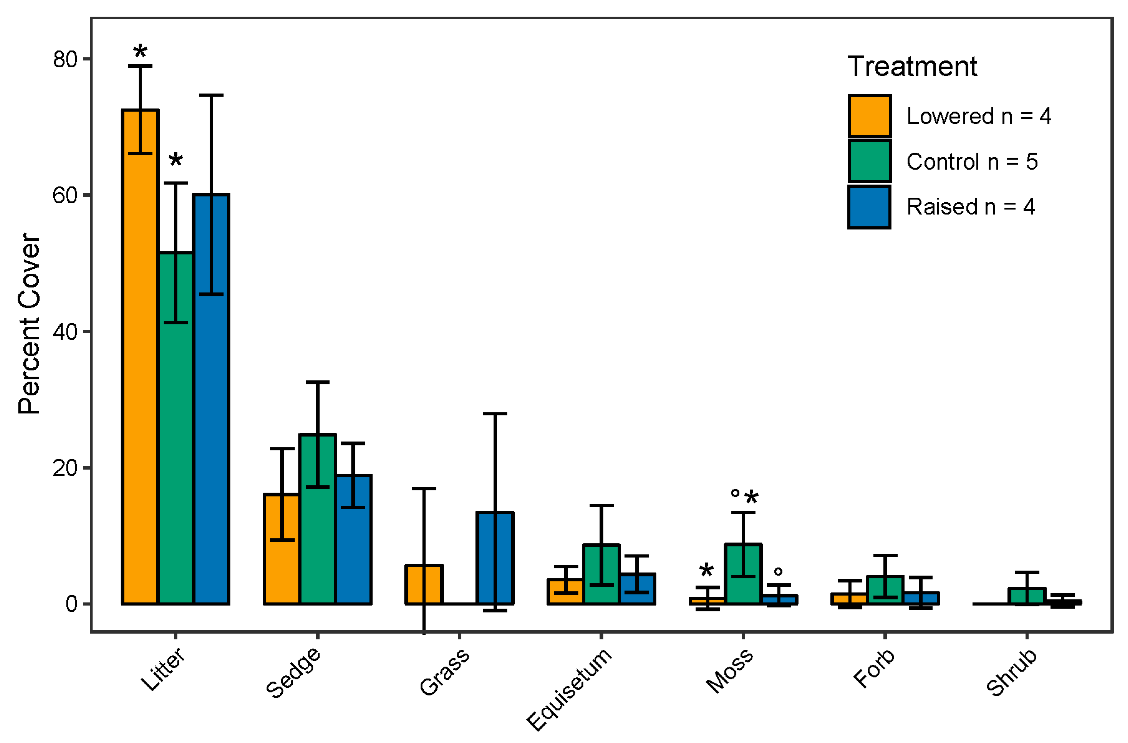
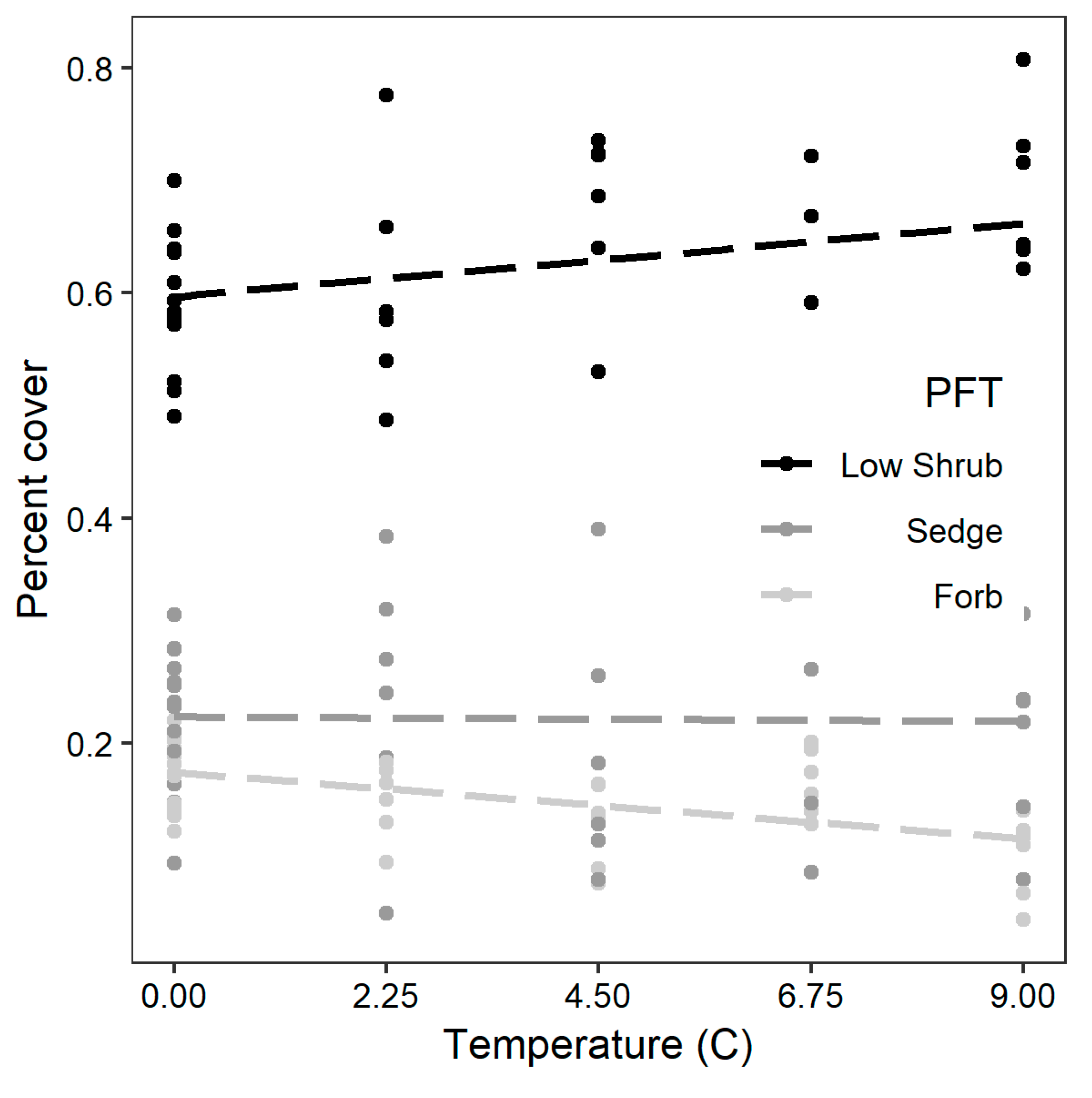
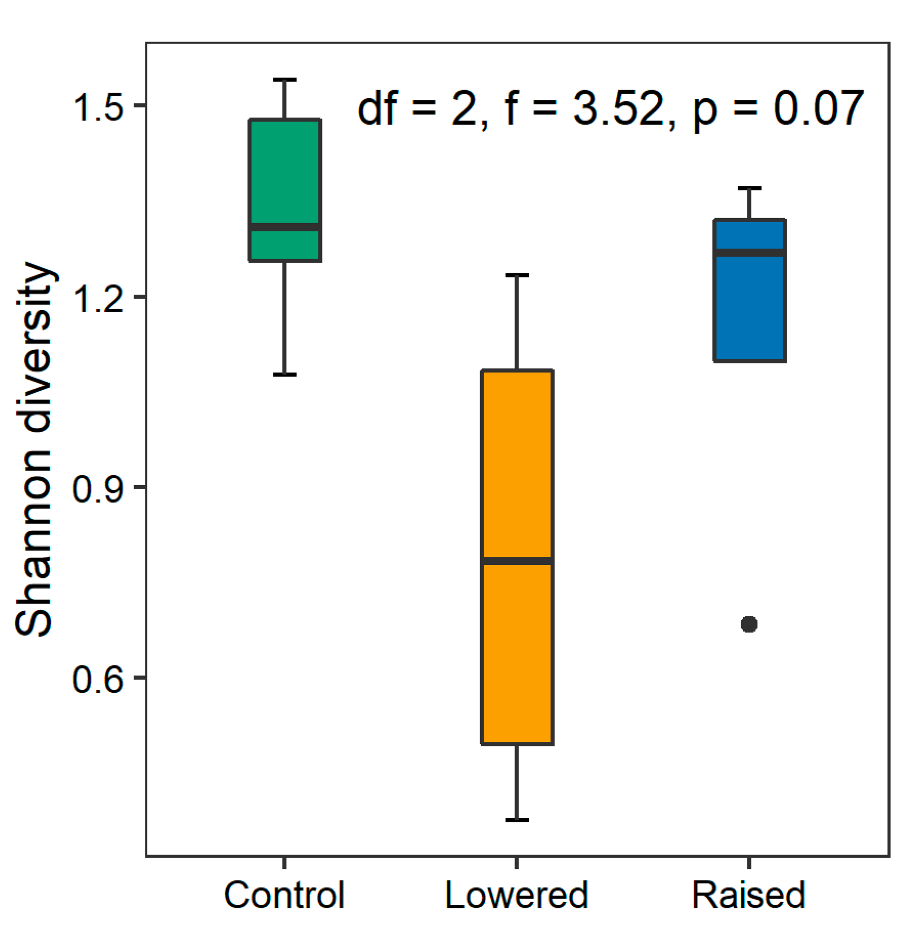
3.1. Response of Plant Functional Composition and Species Diversity to Experimental Maniuplation
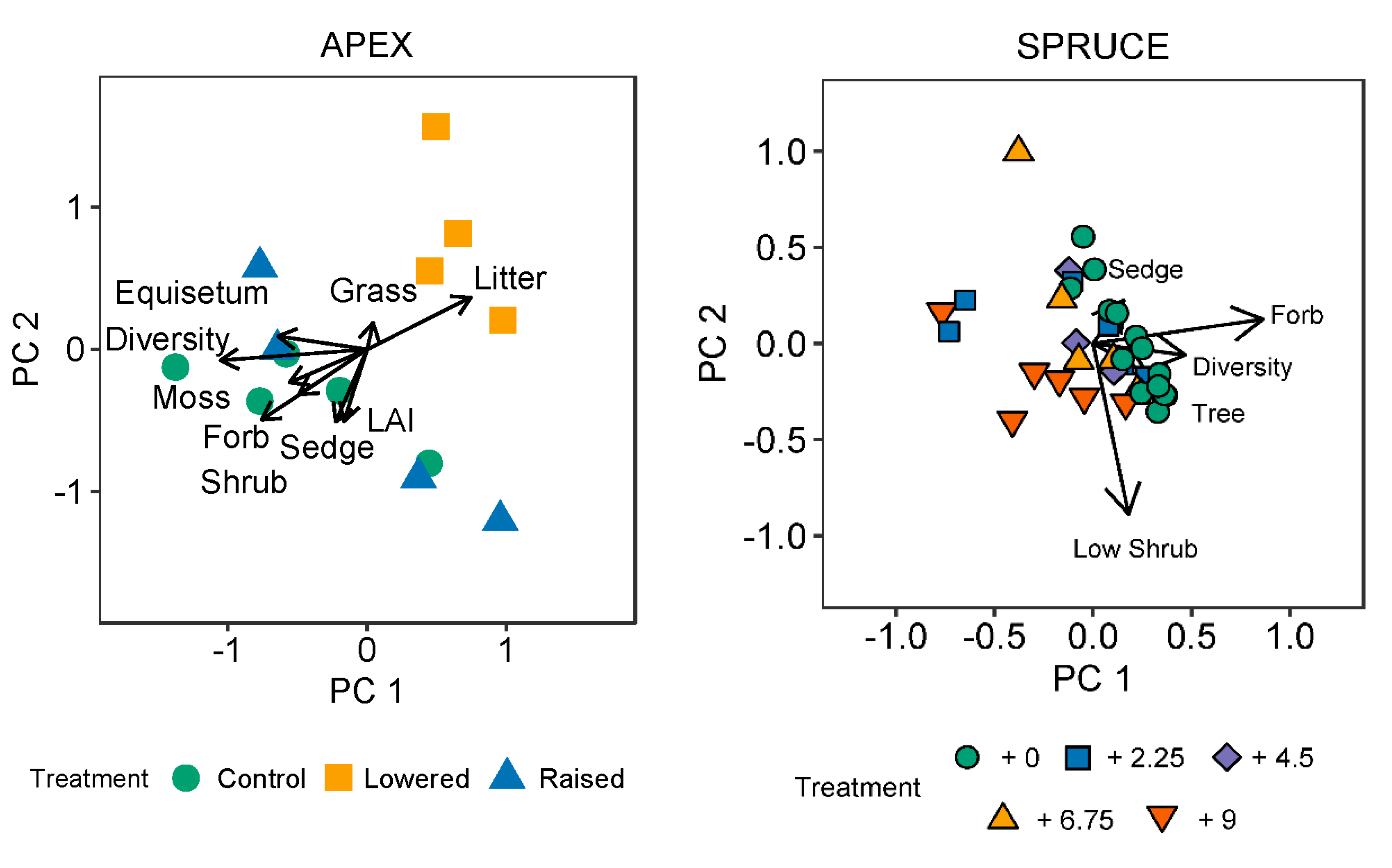
3.2. Relationship between Community Composition and Spectral Response
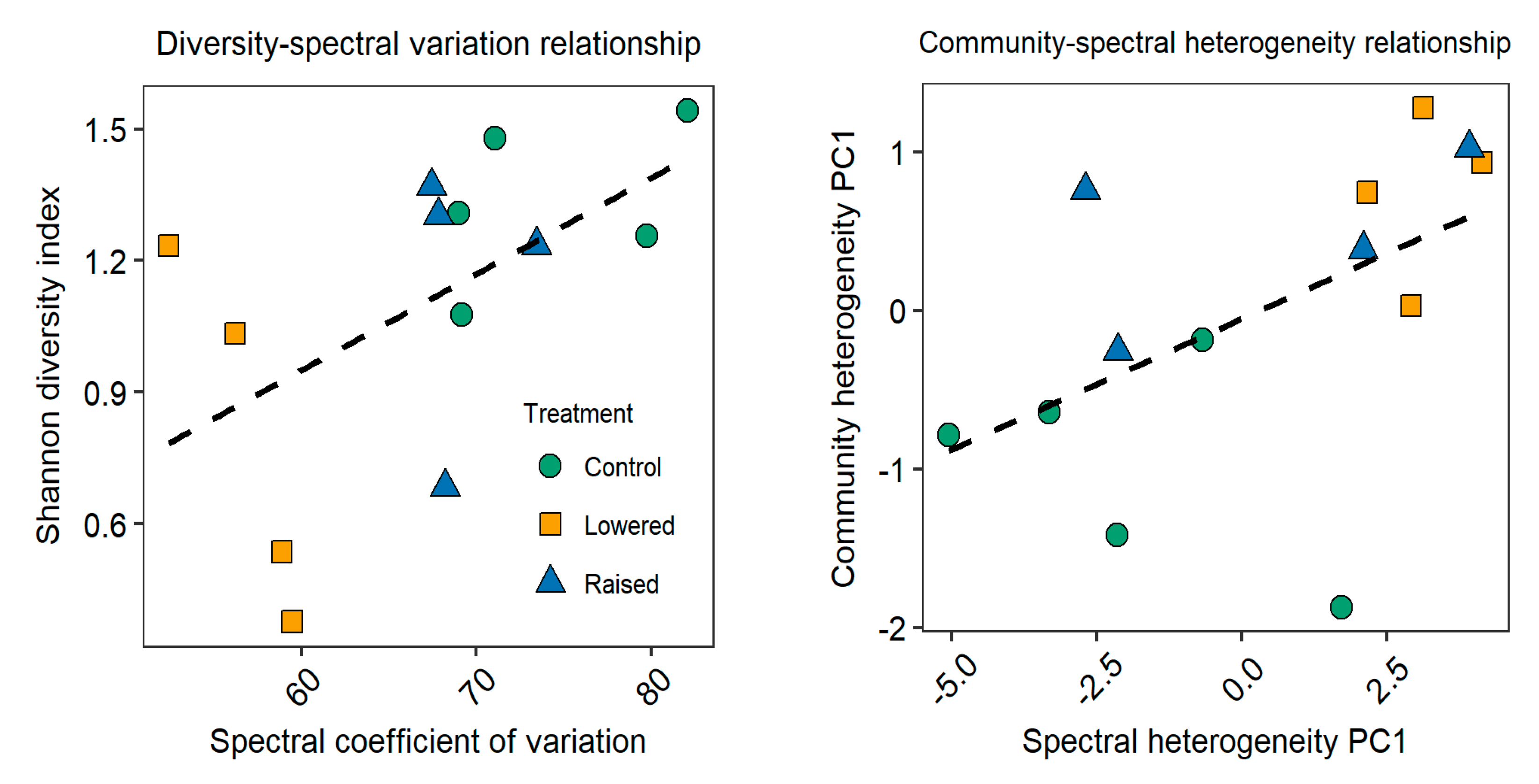
3.3. Relationship between Species Diversity and Spectral Variation
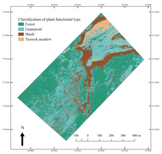
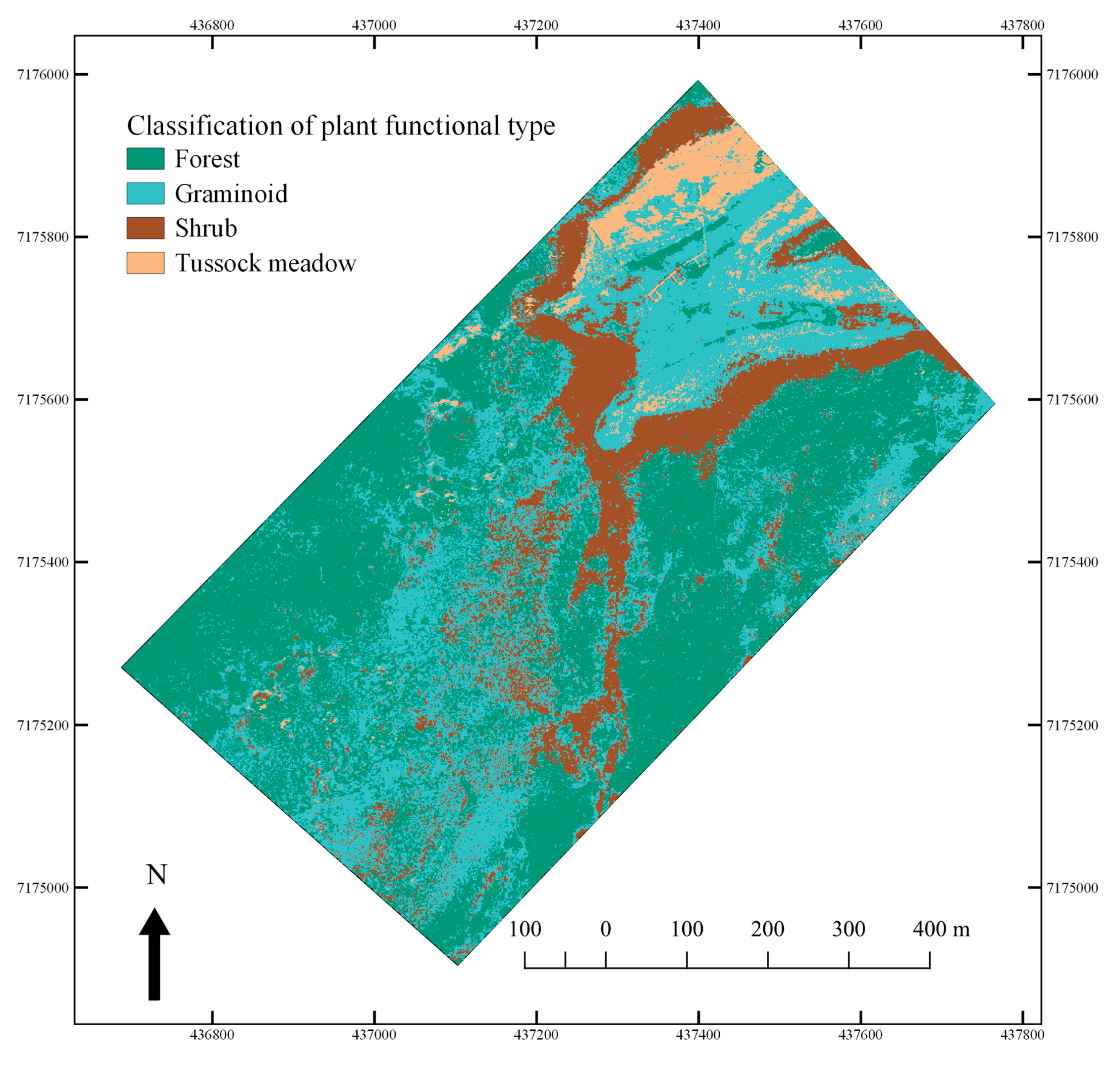
3.4. Hyperspectral Image Analysis—Mapping of PFTs
4. Discussion
4.1. Hyperspectral Remote Sensing of Peatland Response to Climate Change
4.2. Remote Sensing of Boreal Peatland Species Diversity
4.3. Hyperspectral Characterization and Mapping of Plant Functional Types
5. Conclusions
Supplementary Materials
Author Contributions
Funding
Acknowledgments
Conflicts of Interest
References
- Tape, K.; Sturm, M.; Racine, C. The evidence for shrub expansion in Northern Alaska and the Pan-Arctic. Glob. Chang. Biol. 2006, 12, 686–702. [Google Scholar] [CrossRef]
- Myers-Smith, I.H.; Harden, J.W.; Wilmking, M.; Fuller, C.C.; McGuire, A.D.; Chapin, F.S.I. Wetland Succession in a Permafrost Collapse: Interations between Fire and Thermokarst. Biogeosciences 2008, 5, 1273–1286. [Google Scholar] [CrossRef]
- Myers-Smith, I.H.; Elmendorf, S.C.; Beck, P.S.A.; Wilmking, M.; Hallinger, M.; Blok, D.; Tape, K.D.; Rayback, S.A.; Macias-Fauria, M.; Forbes, B.C.; et al. Climate sensitivity of shrub growth across the tundra biome. Nat. Clim. Chang. 2015, 5, 887–891. [Google Scholar] [CrossRef]
- Myers-Smith, I.H.; Forbes, B.C.; Wilmking, M.; Hallinger, M.; Lantz, T.; Blok, D.; Tape, K.D.; Macias-Fauria, M.; Sass-Klaassen, U.; Lévesque, E.; et al. Shrub Expansion in Tundra Ecosystems: Dynamics, Impacts and Research Priorities. Environ. Res. Lett. 2011, 6, 045509. [Google Scholar] [CrossRef]
- Johnstone, J.F.; Hollingsworth, T.N.; Mack, M.C.; Turetsky, M.; Chapin, F.S.; Romanovsky, V. Fire, climate change, and forest resilience in interior Alaska This article is one of a selection of papers from The Dynamics of Change in Alaska’s Boreal Forests: Resilience and Vulnerability in Response to Climate Warming. Can. J. For. Res. 2010, 40, 1302–1312. [Google Scholar] [CrossRef]
- Weintraub, M.N.; Schimel, J.P. Nitrogen Cycling and the Spread of Shrubs Control Changes in the Carbon Balance of Arctic Tundra Ecosystems. BioScience 2005, 55, 408–415. [Google Scholar] [CrossRef]
- Mack, M.C.; Schuur, E.A.G.; Bret-Harte, M.S.; Shaver, G.R.; Chapin, F.S. Ecosystem carbon storage in arctic tundra reduced by long-term nutrient fertilization. Nature 2004, 431, 440–443. [Google Scholar] [CrossRef] [PubMed]
- Douglas, T.A.; Jones, M.C.; Hiemstra, C.A.; Arnold, J.R. Sources and sinks of carbon in boreal ecosystems of interior Alaska: A review. Elem. Sci. Anth. 2014, 2. [Google Scholar] [CrossRef]
- Van Hemert, C.; Flint, P.L.; Udevitz, M.S.; Koch, J.C.; Atwood, T.C.; Oakley, K.L.; Pearce, J.M. Forecasting Wildlife Response to Rapid Warming in the Alaskan Arctic. BioScience 2015, 65, 718–728. [Google Scholar] [CrossRef]
- Berteaux, D.; Gauthier, G.; Domine, F.; Ims, R.A.; Lamoureux, S.F.; Lévesque, E.; Yoccoz, N. Effects of Changing Permafrost and Snow Conditions on Tundra Wildlife: Critical Places and Times. Arct. Sci. 2016, 3, 65–90. [Google Scholar] [CrossRef]
- Chapin, F.S., III; Sommerkorn, M.; Robards, M.D.; Hillmer-Pegram, K. Ecosystem stewardship: A resilience framework for arctic conservation. Glob. Environ. Chang. 2015, 34, 207–217. [Google Scholar] [CrossRef]
- Horstkotte, T.; Utsi, T.A.; Larsson-Blind, Å.; Burgess, P.; Johansen, B.; Käyhkö, J.; Oksanen, L.; Forbes, B.C. Human–Animal Agency in Reindeer Management: Sámi Herders’ Perspectives on Vegetation Dynamics under Climate Change. Ecosphere 2017, 8, e01931. [Google Scholar] [CrossRef]
- Gorham, E. Northern Peatlands: Role in the Carbon Cycle and Probable Responses to Climatic Warming. Ecol. Appl. 1991, 1, 182–195. [Google Scholar] [CrossRef] [PubMed]
- Yu, Z.; Loisel, J.; Brosseau, D.P.; Beilman, D.W.; Hunt, S.J. Global peatland dynamics since the Last Glacial Maximum. Geophys. Res. Lett. 2010, 37. [Google Scholar] [CrossRef]
- Treat, C.C.; Kleinen, T.; Broothaerts, N.; Dalton, A.S.; Dommain, R.; Douglas, T.A.; Drexler, J.Z.; Finkelstein, S.A.; Grosse, G.; Hope, G.; et al. Widespread global peatland establishment and persistence over the last 130,000 y. Proc. Natl. Acad. Sci. USA 2019, 116, 4822–4827. [Google Scholar] [CrossRef] [PubMed]
- Harris, A.; Gamon, J.A.; Pastorello, G.; Wong, C. Retrieval of the photochemical reflectance index for assessing xanthophyll cycle activity: A comparison of near-surface optical sensors. Biogeosciences 2014, 11, 6277–6292. [Google Scholar] [CrossRef]
- Erudel, T.; Fabre, S.; Houet, T.; Mazier, F.; Briottet, X. Criteria Comparison for Classifying Peatland Vegetation Types Using In Situ Hyperspectral Measurements. Remote Sens. 2017, 9, 748. [Google Scholar] [CrossRef]
- Kattge, J.; Díaz, S.; Lavorel, S.; Prentice, I.C.; Leadley, P.; Bonisch, G.; Garnier, E.; Westoby, M.; Reich, P.B.; Wright, I.J.; et al. TRY—A global database of plant traits. Glob. Chang. Biol. 2011, 17, 2905–2935. [Google Scholar] [CrossRef]
- Jetz, W.; Cavender-Bares, J.; Pavlick, R.; Schimel, D.; Davis, F.W.; Asner, G.P.; Guralnick, R.; Kattge, J.; Latimer, A.M.; Moorcroft, P.; et al. Monitoring plant functional diversity from space. Nat. Plants 2016, 2, 16024. [Google Scholar] [CrossRef] [PubMed]
- Weltzin, J.F.; Bridgham, S.D.; Pastor, J.; Chen, J.; Harth, C. Potential effects of warming and drying on peatland plant community composition. Glob. Chang. Biol. 2003, 9, 141–151. [Google Scholar] [CrossRef]
- Weltzin, J.F.; Pastor, J.; Harth, C.; Bridgham, S.D.; Updegraff, K.; Chapin, C.T. Response of bog and fen plant communities to warming and water-table manipulations. Ecology 2000, 81, 3464–3478. [Google Scholar] [CrossRef]
- Churchill, A.C.; Turetsky, M.R.; McGuire, A.D.; Hollingsworth, T.N. Response of Plant Community Structure and Primary Productivity to Experimental Drought and Flooding in an Alaskan Fen. Can. J. For. Res. 2014, 45, 185–193. [Google Scholar] [CrossRef]
- Dieleman, C.M.; Branfireun, B.A.; McLaughlin, J.W.; Lindo, Z. Climate Change Drives a Shift in Peatland Ecosystem Plant Community: Implications for Ecosystem Function and Stability. Glob. Chang. Biol. 2015, 21, 388–395. [Google Scholar] [CrossRef] [PubMed]
- Radu, D.D.; Duval, T.P. Precipitation frequency alters peatland ecosystem structure and CO2 exchange: Contrasting effects on moss, sedge, and shrub communities. Glob. Chang. Biol. 2018, 24, 2051–2065. [Google Scholar] [CrossRef] [PubMed]
- McPartland, M.Y.; Kane, E.S.; Falkowski, M.J.; Kolka, R.; Turetsky, M.R.; Palik, B.; Montgomery, R.A. The Response of Boreal Peatland Community Composition and NDVI to Hydrologic Change, Warming and Elevated Carbon Dioxide. Glob. Chang. Biol. 2019, 25, 93–107. [Google Scholar] [CrossRef]
- Olefeldt, D.; Euskirchen, E.S.; Harden, J.; Kane, E.; McGuire, A.D.; Waldrop, M.P.; Turetsky, M.R. A decade of boreal rich fen greenhouse gas fluxes in response to natural and experimental water table variability. Glob. Chang. Biol. 2017, 23, 2428–2440. [Google Scholar] [CrossRef] [PubMed]
- Christensen, T.R.; Johansson, T.; Åkerman, H.J.; Mastepanov, M.; Svensson, B.H.; Malmer, N.; Friborg, T.; Crill, P. Thawing sub-arctic permafrost: Effects on vegetation and methane emissions. Geophys. Res. Lett. 2004, 31. [Google Scholar] [CrossRef]
- Goud, E.M.; Moore, T.R.; Roulet, N.T. Predicting Peatland Carbon Fluxes from Non-Destructive Plant Traits. Funct. Ecol. 2018, 31, 1824–1833. [Google Scholar] [CrossRef]
- Chapin, F.S.; Hobbie, S.E.; Zhong, H.; Bret-Harte, M.S. Plant functional types as predictors of transient responses of arctic vegetation to global change. J. Veg. Sci. 1996, 7, 347–358. [Google Scholar] [CrossRef]
- Pielke, R.; Baldocchi, D.; Hobbie, S.E.; Roulet, N.; Eugster, W.; Kasischke, E.; Rastetter, E.; Zimov, S.A.; Running, S.W.; Chapin, F.S.; et al. Arctic and boreal ecosystems of western North America as components of the climate system. Glob. Chang. Biol. 2000, 6, 211–223. [Google Scholar] [CrossRef]
- Turner, W. Sensing Biodiversity. Science 2014, 346, 301–302. [Google Scholar] [CrossRef] [PubMed]
- Goetz, A.F.; Vane, G.; Solomon, J.E.; Rock, B.N. Imaging Spectrometry for Earth Remote Sensing. Science 1985, 228, 1147–1153. [Google Scholar] [CrossRef] [PubMed]
- Ustin, S.L.; Gamon, J.A. Remote sensing of plant functional types. New Phytol. 2010, 186, 795–816. [Google Scholar] [CrossRef] [PubMed]
- Ustin, S.L.; Roberts, D.A.; Gamon, J.A.; Asner, G.P.; Green, R.O. Using Imaging Spectroscopy to Study Ecosystem Processes and Properties. BioScience 2004, 54, 523–534. [Google Scholar] [CrossRef]
- Lichtenthaler, H.K.; Gitelson, A.; Lang, M. Non-Destructive Determination of Chlorophyll Content of Leaves of a Green and an Aurea Mutant of Tobacco by Reflectance Measurements. J. Plant Physiol. 1996, 148, 483–493. [Google Scholar] [CrossRef]
- Sims, D.A.; Gamon, J.A. Relationships between leaf pigment content and spectral reflectance across a wide range of species, leaf structures and developmental stages. Remote Sens. Environ. 2002, 81, 337–354. [Google Scholar] [CrossRef]
- Blackburn, G.A. Hyperspectral Remote Sensing of Plant Pigments. J. Exp. Bot. 2007, 58, 855–867. [Google Scholar] [CrossRef]
- Serbin, S.P.; Singh, A.; McNeil, B.E.; Kingdon, C.C.; Townsend, P.A. Spectroscopic determination of leaf morphological and biochemical traits for northern temperate and boreal tree species. Ecol. Appl. 2014, 24, 1651–1669. [Google Scholar] [CrossRef]
- Martin, M.E.; Aber, J.D. High spectral resolution remote sensing of forest canopy lignin, nitrogen, and ecosystem processes. Ecol. Appl. 1997, 7, 431–443. [Google Scholar] [CrossRef]
- Knyazikhin, Y.; Schull, M.A.; Stenberg, P.; Mõttus, M.; Rautiainen, M.; Yang, Y.; Marshak, A.; Carmona, P.L.; Kaufmann, R.K.; Lewis, P.; et al. Hyperspectral Remote Sensing of Foliar Nitrogen Content. Proc. Natl. Acad. Sci. USA 2013, 110, 811–812. [Google Scholar] [CrossRef]
- Peñuelas, J.; Pinol, J.; Ogaya, R.; Filella, I. Estimation of plant water concentration by the reflectance Water Index WI (R900/R970). Int. J. Remote Sens. 1997, 18, 2869–2875. [Google Scholar] [CrossRef]
- Schweiger, A.K.; Cavender-Bares, J.; Townsend, P.A.; Hobbie, S.E.; Madritch, M.D.; Wang, R.; Tilman, D.; Gamon, J.A. Plant spectral diversity integrates functional and phylogenetic components of biodiversity and predicts ecosystem function. Nat. Ecol. Evol. 2018, 2, 976–982. [Google Scholar] [CrossRef] [PubMed]
- Turner, W.; Spector, S.; Gardiner, N.; Fladeland, M.; Sterling, E.; Steininger, M. Remote sensing for biodiversity science and conservation. Trends Ecol. Evol. 2003, 18, 306–314. [Google Scholar] [CrossRef]
- Tilman, D. The Influence of Functional Diversity and Composition on Ecosystem Processes. Science 1997, 277, 1300–1302. [Google Scholar] [CrossRef]
- Walker, M.D.; Wahren, C.H.; Hollister, R.D.; Henry, G.H.R.; Ahlquist, L.E.; Alatalo, J.M.; Bret-Harte, M.S.; Calef, M.P.; Callaghan, T.V.; Carroll, A.B.; et al. Plant community responses to experimental warming across the tundra biome. Proc. Natl. Acad. Sci. USA 2006, 103, 1342–1346. [Google Scholar] [CrossRef]
- Pajunen, A.; Oksanen, J.; Virtanen, R. Impact of shrub canopies on understorey vegetation in western Eurasian tundra. J. Veg. Sci. 2011, 22, 837–846. [Google Scholar] [CrossRef]
- Reich, P.B.; Tilman, D.; Isbell, F.; Mueller, K.; Hobbie, S.E.; Flynn, D.F.B.; Eisenhauer, N. Impacts of Biodiversity Loss Escalate Through Time as Redundancy Fades. Science 2012, 336, 589–592. [Google Scholar] [CrossRef]
- Ward, S.E.; Ostle, N.J.; Oakley, S.; Quirk, H.; Henrys, P.A.; Bardgett, R.D. Warming effects on greenhouse gas fluxes in peatlands are modulated by vegetation composition. Ecol. Lett. 2013, 16, 1285–1293. [Google Scholar] [CrossRef]
- Wang, R.; Gamon, J.A.; Emmerton, C.A.; Li, H.; Nestola, E.; Pastorello, G.Z.; Menzer, O. Integrated Analysis of Productivity and Biodiversity in a Southern Alberta Prairie. Remote Sens. 2016, 8, 214. [Google Scholar] [CrossRef]
- Wang, R.; Gamon, J.A.; Schweiger, A.K.; Cavender-Bares, J.; Townsend, P.A.; Zygielbaum, A.I.; Kothari, S. Influence of species richness, evenness, and composition on optical diversity: A simulation study. Remote Sens. Environ. 2018, 211, 218–228. [Google Scholar] [CrossRef]
- Palmer, M.W.; Earls, P.G.; Hoagland, B.W.; White, P.S.; Wohlgemuth, T. Quantitative tools for perfecting species lists. Environmetrics 2002, 13, 121–137. [Google Scholar] [CrossRef]
- Rocchini, D. Effects of spatial and spectral resolution in estimating ecosystem α-diversity by satellite imagery. Remote Sens. Environ. 2007, 111, 423–434. [Google Scholar] [CrossRef]
- Rocchini, D.; Balkenhol, N.; Carter, G.A.; Foody, G.M.; Gillespie, T.W.; He, K.S.; Kark, S.; Levin, N.; Lucas, K.; Luoto, M.; et al. Remotely sensed spectral heterogeneity as a proxy of species diversity: Recent advances and open challenges. Ecol. Inform. 2010, 5, 318–329. [Google Scholar] [CrossRef]
- Baldeck, C.A.; Asner, G.P. Estimating Vegetation Beta Diversity from Airborne Imaging Spectroscopy and Unsupervised Clustering. Remote Sens. 2013, 5, 2057–2071. [Google Scholar] [CrossRef]
- Gould, W. Remote sensing of vegetation, plant species richness, and regional biodiversity hotspots. Ecol. Appl. 2000, 10, 1861–1870. [Google Scholar] [CrossRef]
- Carter, G.A.; Knapp, A.K.; Anderson, J.E.; Hoch, G.A.; Smith, M.D. Indicators of plant species richness in AVIRIS spectra of a mesic grassland. Remote Sens. Environ. 2005, 98, 304–316. [Google Scholar] [CrossRef]
- Levin, N.; Shmida, A.; Levanoni, O.; Tamari, H.; Kark, S. Predicting mountain plant richness and rarity from space using satellite-derived vegetation indices. Divers. Distrib. 2007, 13, 692–703. [Google Scholar] [CrossRef]
- Lucas, K.; Carter, G. The use of hyperspectral remote sensing to assess vascular plant species richness on Horn Island, Mississippi. Remote Sens. Environ. 2008, 112, 3908–3915. [Google Scholar] [CrossRef]
- Oldeland, J.; Wesuls, D.; Rocchini, D.; Schmidt, M.; Jürgens, N. Does using species abundance data improve estimates of species diversity from remotely sensed spectral heterogeneity? Ecol. Indic. 2010, 10, 390–396. [Google Scholar] [CrossRef]
- Pereira, H.M.; Ferrier, S.; Walters, M.; Geller, G.N.; Jongman, R.H.G.; Scholes, R.J.; Bruford, M.W.; Brummitt, N.; Butchart, S.H.M.; Cardoso, A.C.; et al. Essential Biodiversity Variables. Science 2013, 339, 277–278. [Google Scholar] [CrossRef]
- Proença, V.; Martin, L.J.; Pereira, H.M.; Fernandez, M.; McRae, L.; Belnap, J.; Böhm, M.; Brummitt, N.; García-Moreno, J.; Gregory, R.D.; et al. Global biodiversity monitoring: From data sources to Essential Biodiversity Variables. Biol. Conserv. 2017, 213, 256–263. [Google Scholar] [CrossRef]
- Vihervaara, P.; Auvinen, A.-P.; Mononen, L.; Törmä, M.; Ahlroth, P.; Anttila, S.; Böttcher, K.; Forsius, M.; Heino, J.; Heliölä, J.; et al. How Essential Biodiversity Variables and Remote Sensing Can Help National Biodiversity Monitoring. Glob. Ecol. Conserv. 2017, 10, 43–59. [Google Scholar] [CrossRef]
- Hanson, P.J.; Riggs, J.S.; Nettles, W.R.; Phillips, J.R.; Krassovski, M.B.; Hook, L.A.; Gu, L.; Richardson, A.D.; Aubrecht, D.M.; Ricciuto, D.M.; et al. Attaining whole-ecosystem warming using air and deep-soil heating methods with an elevated CO2 atmosphere. Biogeosciences 2017, 14, 861–883. [Google Scholar] [CrossRef]
- Jonasson, S. Evaluation of the Point Intercept Method for the Estimation of Plant Biomass. Oikos 1988, 52, 101–106. [Google Scholar] [CrossRef]
- ASD. Fieldspec 3 User Manual; ASD Inc.: Boulder, CO, USA, 2007. [Google Scholar]
- Herweg, J.A.; Kerekes, J.P.; Weatherbee, O.; Messinger, D.; Van Aardt, J.; Ientilucci, E.; Ninkov, Z.; Faulring, J.; Raqueno, N.; Meola, J. SpecTIR hyperspectral airborne Rochester experiment data collection campaign. SPIE Def. Secur. Sens. 2012, 8390, 839028. [Google Scholar] [CrossRef]
- Kruse, F.; Lefkoff, A.; Boardman, J.; Heidebrecht, K.; Shapiro, A.; Barloon, P.; Goetz, A. The spectral image processing system (SIPS)—Interactive visualization and analysis of imaging spectrometer data. Remote Sens. Environ. 1993, 44, 145–163. [Google Scholar] [CrossRef]
- Anderson, J.E.; Douglas, T.A.; Barbato, R.A.; Saari, S.; Jones, R.M. Vegetation Mapping and Seasonal Thaw Estimates in Interior Alaska Permafrost. Remote Sens. Environ. In review.
- Nakagawa, S.; Schielzeth, H. A General and Simple Method for Obtaining R2 from Generalized Linear Mixed-Effects Models. Methods Ecol. Evol. 2013, 4, 133–142. [Google Scholar] [CrossRef]
- Gotelli, N.J.; Ellison, A.M. A Primer of Ecological Statistics, 2nd ed.; Sinauer Associates Is an Imprint of Oxford University Press: Sunderland, MA, USA, 2012; ISBN 978-1-60535-064-6. [Google Scholar]
- Oksanen, J.; Blanchet, F.G.; Friendly, M.; Kindt, R.; Legendre, P.; McGlinn, D.; Minchin, P.R.; O’Hara, R.B.; Simpson, G.L.; Solymos, P.; et al. vegan: Community Ecology Package. R package version 2.4-4. 2017. Available online: https://CRAN.R-project.org/package=vegan (accessed on 16 July 2019).
- Zuur, A.F.; Ieno, E.N.; Smith, G.M. (Eds.) Principal component analysis and redundancy analysis. In Analysing Ecological Data; Statistics for Biology and Health; Springer: New York, NY, USA, 2007; pp. 193–224. [Google Scholar]
- Legendre, P.; Legendre, L.F.J. Numerical Ecology; Elsevier: Oxford, UK, 2012; ISBN 978-0-444-53869-7. [Google Scholar]
- Harsanyi, J.C.; Chang, C.-I. Hyperspectral image classification and dimensionality reduction: An orthogonal subspace projection approach. IEEE Trans. Geosci. Remote. Sens. 1994, 32, 779–785. [Google Scholar] [CrossRef]
- Li, W.; Prasad, S.; Fowler, J.E.; Bruce, L.M. Locality-Preserving Dimensionality Reduction and Classification for Hyperspectral Image Analysis. IEEE Trans. Geosci. Remote Sens. 2012, 50, 1185–1198. [Google Scholar] [CrossRef]
- Li, H.; Reynolds, J.F. On Definition and Quantification of Heterogeneity. Oikos 1995, 73, 280–284. [Google Scholar] [CrossRef]
- Breiman, L. Random forests. Mach. Learn. 2001, 45, 5–32. [Google Scholar] [CrossRef]
- Liaw, A.; Wiener, M. Classification and Regression by RandomForest. R News 2003, 2, 18–22. [Google Scholar]
- Bivand, R.; Keitt, T.; Rowlingson, B. rgdal: Bindings for the ‘Geospatial’ Data Abstraction Library. R package version 1.2-16. 2017. Available online: https://CRAN.R-project.org/package=rgdal (accessed on 16 July 2019).
- Evans, J.S.; Murphy, M.A.; Holden, Z.A.; Cushman, S.A. Modeling Species Distribution and Change Using Random Forest. In Predictive Species and Habitat Modeling in Landscape Ecology: Concepts and Applications; Springer: Drew, CA, USA, 2011; ISBN 978-1-4419-7390-0. [Google Scholar]
- Mitchell, M.W. Bias of the Random Forest Out-of-Bag (OOB) Error for Certain Input Parameters. Open J. Stat. 2011, 1, 205–211. [Google Scholar] [CrossRef]
- QGIS Development Team. QGIS Geographic Information System. Open Source Geospatial Foundation Project. 2018. Available online: http://qgis.osgeo.org (accessed on 16 July 2019).
- Boelman, N.T.; Stieglitz, M.; Rueth, H.M.; Sommerkorn, M.; Griffin, K.L.; Shaver, G.R.; Gamon, J.A. Response of NDVI, biomass, and ecosystem gas exchange to long-term warming and fertilization in wet sedge tundra. Oecologia 2003, 135, 414–421. [Google Scholar] [CrossRef] [PubMed]
- Chivers, M.R.; Turetsky, M.R.; Waddington, J.M.; Harden, J.W.; McGuire, A.D. Effects of Experimental Water Table and Temperature Manipulations on Ecosystem CO2 Fluxes in an Alaskan Rich Fen. Ecosystems 2009, 12, 1329–1342. [Google Scholar] [CrossRef]
- Meingast, K.M.; Falkowski, M.J.; Kane, E.S.; Potvin, L.R.; Benscoter, B.W.; Smith, A.M.; Bourgeau-Chavez, L.L.; Miller, M.E. Spectral detection of near-surface moisture content and water-table position in northern peatland ecosystems. Remote Sens. Environ. 2014, 152, 536–546. [Google Scholar] [CrossRef]
- Schmidtlein, S.; Feilhauer, H.; Bruelheide, H. Mapping Plant Strategy Types Using Remote Sensing. J. Veg. Sci. 2012, 23, 395–405. [Google Scholar] [CrossRef]
- Harris, A.; Charnock, R.; Lucas, R. Hyperspectral remote sensing of peatland floristic gradients. Remote Sens. Environ. 2015, 162, 99–111. [Google Scholar] [CrossRef]
- Chapin, F.S., III; Shaver, G.R.; Giblin, A.E.; Nadelhoffer, K.J.; Laundre, J.A. Responses of Arctic Tundra to Experimental and Observed Changes in Climate. Ecology 1995, 76, 694–711. [Google Scholar] [CrossRef]
- Shaver, G.R.; Bret-Harte, M.S.; Chapin, F.S. Primary and secondary stem growth in arctic shrubs: Implications for community response to environmental change. J. Ecol. 2002, 90, 251–267. [Google Scholar] [CrossRef]
- Bratsch, S.N.; Epstein, H.E.; Buchhorn, M.; Walker, D.A. Differentiating among Four Arctic Tundra Plant Communities at Ivotuk, Alaska Using Field Spectroscopy. Remote Sens. 2016, 8, 51. [Google Scholar] [CrossRef]
- Poulin, M.F.; Careau, D.; Rochefort, L.; DesRochers, A. From Satellite Imagery to Peatland Vegetation Diversity: How Reliable Are Habitat Maps? Conserv. Ecol. 2002, 6. [Google Scholar] [CrossRef]
- Cabezas, J.; Galleguillos, M.; Perez-Quezada, J.F. Predicting Vascular Plant Richness in a Heterogeneous Wetland Using Spectral and Textural Features and a Random Forest Algorithm. IEEE Geosci. Remote Sens. Lett. 2016, 13, 1–5. [Google Scholar] [CrossRef]
- Lopatin, J.; Kattenborn, T.; Galleguillos, M.; Perez-Quezada, J.F.; Schmidtlein, S. Using aboveground vegetation attributes as proxies for mapping peatland belowground carbon stocks. Remote Sens. Environ. 2019, 231, 111217. [Google Scholar] [CrossRef]
- Whittaker, R.H. Evolution and Measurement of Species Diversity. Taxon 1972, 21, 213–251. [Google Scholar] [CrossRef]
- Baldeck, C.A.; Colgan, M.S.; Féret, J.-B.; Levick, S.R.; Martin, R.E.; Asner, G.P.; Asner, G. Landscape-scale variation in plant community composition of an African savanna from airborne species mapping. Ecol. Appl. 2014, 24, 84–93. [Google Scholar] [CrossRef]
- Carlson, K.M.; Asner, G.P.; Hughes, R.F.; Ostertag, R.; Martin, R.E. Hyperspectral Remote Sensing of Canopy Biodiversity in Hawaiian Lowland Rainforests. Ecosystems 2007, 10, 536–549. [Google Scholar] [CrossRef]
- Féret, J.-B.; Asner, G.P. Mapping Tropical Forest Canopy Diversity Using High-Fidelity Imaging Spectroscopy. Ecological Applications 2014, 24(6), 1289–1296. [Google Scholar] [CrossRef]
- Feilhauer, H.; Faude, U.; Schmidtlein, S. Combining Isomap ordination and imaging spectroscopy to map continuous floristic gradients in a heterogeneous landscape. Remote Sens. Environ. 2011, 115, 2513–2524. [Google Scholar] [CrossRef]
- Kattenborn, T.; Fassnacht, F.E.; Schmidtlein, S. Differentiating Plant Functional Types Using Reflectance: Which Traits Make the Difference? Remote Sens. Ecol. Conserv. 2019, 5, 5–19. [Google Scholar] [CrossRef]
- Miller, C.E.; Green, R.O.; Thompson, D.R.; Thorpe, A.K.; Eastwood, M.; Mccubbin, I.B.; Olson-Duvall, W.; Bernas, M.; Sarture, C.M.; Nolte, S.; et al. ABoVE: Hyperspectral Imagery from AVIRIS-NG, Alaskan and Canadian Arctic, 2017–2018. ORNL DAAC 2018. [Google Scholar] [CrossRef]
- Lee, C.M.; Cable, M.L.; Hook, S.J.; Green, R.O.; Ustin, S.L.; Mandl, D.J.; Middleton, E.M. An Introduction to the NASA Hyperspectral InfraRed Imager (HyspIRI) Mission and Preparatory Activities. Remote Sens. Environ. 2015, 167, 6–19. [Google Scholar] [CrossRef]
- Kampe, T.U.; Johnson, B.R.; Kuester, M.A.; Keller, M. NEON: The first continental-scale ecological observatory with airborne remote sensing of vegetation canopy biochemistry and structure. J. Appl. Remote Sens. 2010, 4, 043510. [Google Scholar] [CrossRef]


| APEX | SPRUCE | |
|---|---|---|
| Peatland type | Rich fen | Ombrotrophic bog |
| Location | Alaska, USA | Minnesota, USA |
| Experimental design | Water table manipulation with 120 m2 control, lowered and raised treatments | Regression-based factorial between increasing temperature and CO2 level |
| Vegetation sampling | Point bar laser survey method | 2 m2 sampling frame method |
| Spectral reflectance | ASD Fieldspec Pro | Unispec DC |
| SPRUCE | APEX | ||
|---|---|---|---|
| PFT | Species | PFT | Species |
| Forb | Drosera rotundifolia | Equisetum | Equisetum fluviatile |
| Forb | Maianthemum trifolium | Forb | Galium trifidum |
| Graminoid | Carex magellanica | Forb | Potamogeton gramineus |
| Graminoid | Carex oligosperma | Graminoid | Calamagrostis canadensis |
| Graminoid | Carex trisperma | Graminoid | Carex loliacea |
| Graminoid | Eriophorum vaginatum | Graminoid | Carex utriculata |
| Graminoid | Eriophorum virginicum | Moss | Sphagnum spp. |
| Shrub | Andromeda polifolia | Shrub | Potentilla palustris |
| Shrub | Chamaedaphne calyculata | ||
| Shrub | Kalmia polifolia | ||
| Shrub | Rhododendron groenlandicum | ||
| Shrub | Vaccinium angustifolium | ||
| Shrub | Vaccinium oxycoccos | ||
| PFT | Sum Sq | Mean Sq | F2, 10 | P |
|---|---|---|---|---|
| Forb | 19.24 | 9.62 | 1.478 | 0.274 |
| Sedge | 182.9 | 91.46 | 2.094 | 0.174 |
| Shrub | 13.36 | 6.73 | 2.724 | 0.114 |
| Equisetum | 68.77 | 34.39 | 2.03 | 0.182 |
| Grass | 402.7 | 201.4 | 1.997 | 0.186 |
| Moss | 182.7 | 91.37 | 8.779 | 0.006 |
| Litter | 980.9 | 490.5 | 4.135 | 0.049 |
| Diversity | 0.650 | 0.33 | 3.516 | 0.07 |
| PFT | Marginal R2 | Conditional R2 | AIC | βTEMP | βCO2 | βTEMP:CO2 |
|---|---|---|---|---|---|---|
| Forb | 0.278 | 0.605 | 342 | −4.444 | −6.143 | 1.170 |
| Sedge | 0.017 | 0.153 | 412 | 0.758 | 15.178 | −3.484 |
| Shrub | 0.155 | 0.251 | 407 | −9.932 | −28.633 | 12.935 |
| Diversity | 0.023 | 0.285 | −37 | −0.003 | 0.024 | −0.005 |
| Variable | PC1 | PC2 | r2 | p |
|---|---|---|---|---|
| Diversity | –0.997 | –0.074 | 0.495 | 0.038 * |
| Equisetum | −0.990 | 0.142 | 0.185 | 0.370 |
| Forbs | −0.839 | −0.545 | 0.151 | 0.458 |
| Sedges | −0.405 | −0.914 | 0.138 | 0.491 |
| Grasses | 0.224 | 0.975 | 0.016 | 0.910 |
| Litter | 0.898 | 0.440 | 0.305 | 0.169 |
| Moss | −0.837 | −0.547 | 0.364 | 0.108 |
| Shrubs | −0.922 | −0.386 | 0.163 | 0.403 |
| LAI | −0.313 | −0.950 | 0.126 | 0.486 |
| Variable | PC1 | PC2 | r2 | p |
|---|---|---|---|---|
| Forbs | 0.926 | 0.377 | 0.244 | 0.011 * |
| Sedges | 0.271 | 0.963 | 0.039 | 0.520 |
| Shrubs | 0.347 | –0.938 | 0.262 | 0.007 ** |
| Trees | 0.906 | −0.423 | 0.033 | 0.581 |
| Diversity | 0.771 | 0.637 | 0.095 | 0.204 |
| Forest | Graminoid | Shrub | Tussock | Class Error | |
|---|---|---|---|---|---|
| Forest | 94 | 5 | 0 | 0 | 0.051 |
| Graminoid fen | 7 | 80 | 2 | 10 | 0.192 |
| Shrub | 1 | 3 | 95 | 0 | 0.040 |
| Tussock Grass | 1 | 9 | 1 | 88 | 0.111 |
| Model Accuracy | Gini/Impurity | ||
|---|---|---|---|
| Band number | Mean Decrease | Band number | Mean decrease |
| 1210 | 7.53 | 1261 | 4.68 |
| 1233 | 6.99 | 1210 | 4.32 |
| 1261 | 6.77 | 1546 | 3.78 |
| 1193 | 6.76 | 1255 | 3.71 |
| 2441 | 6.71 | 1233 | 3.60 |
| 1204 | 6.66 | 1552 | 3.49 |
| 2447 | 6.66 | 1187 | 3.47 |
| 2430 | 6.61 | 1244 | 3.40 |
| 2412 | 6.56 | 1267 | 3.35 |
| 474 | 6.52 | 1215 | 3.29 |
© 2019 by the authors. Licensee MDPI, Basel, Switzerland. This article is an open access article distributed under the terms and conditions of the Creative Commons Attribution (CC BY) license (http://creativecommons.org/licenses/by/4.0/).
Share and Cite
McPartland, M.Y.; Falkowski, M.J.; Reinhardt, J.R.; Kane, E.S.; Kolka, R.; Turetsky, M.R.; Douglas, T.A.; Anderson, J.; Edwards, J.D.; Palik, B.; et al. Characterizing Boreal Peatland Plant Composition and Species Diversity with Hyperspectral Remote Sensing. Remote Sens. 2019, 11, 1685. https://doi.org/10.3390/rs11141685
McPartland MY, Falkowski MJ, Reinhardt JR, Kane ES, Kolka R, Turetsky MR, Douglas TA, Anderson J, Edwards JD, Palik B, et al. Characterizing Boreal Peatland Plant Composition and Species Diversity with Hyperspectral Remote Sensing. Remote Sensing. 2019; 11(14):1685. https://doi.org/10.3390/rs11141685
Chicago/Turabian StyleMcPartland, Mara Y., Michael J. Falkowski, Jason R. Reinhardt, Evan S. Kane, Randy Kolka, Merritt R. Turetsky, Thomas A. Douglas, John Anderson, Jarrod D. Edwards, Brian Palik, and et al. 2019. "Characterizing Boreal Peatland Plant Composition and Species Diversity with Hyperspectral Remote Sensing" Remote Sensing 11, no. 14: 1685. https://doi.org/10.3390/rs11141685
APA StyleMcPartland, M. Y., Falkowski, M. J., Reinhardt, J. R., Kane, E. S., Kolka, R., Turetsky, M. R., Douglas, T. A., Anderson, J., Edwards, J. D., Palik, B., & Montgomery, R. A. (2019). Characterizing Boreal Peatland Plant Composition and Species Diversity with Hyperspectral Remote Sensing. Remote Sensing, 11(14), 1685. https://doi.org/10.3390/rs11141685