Accuracy of Deformation Rates from Campaign GPS Surveys Considering Extended Observation Session and Antenna Set-Up Errors

Abstract

GPS campaign measurements are still in use in the monitoring of ground deformation. Campaign measurements are frequently referred to because installing permanent stations are costly, and they cannot be installed at the desired density. Using the data from the International Global Navigation Satellite Systems (GNSS) Service (IGS) permanent GPS stations, the duration, sampling interval, etc. of the campaign measurements can be simulated. Thus, the contribution of the campaign data to the monitoring of the ground deformation can be evaluated. In this study, we carried out an experiment with the aim of determining the deformation of tectonic plates at the selected IGS stations more accurately considering by extending the observation duration to a full 24 h length. We also made an attempt to take into consideration the antenna set up errors developing a scenario referring to the information available in the literature. We have decimated the continuous data of 40 globally scattered IGS stations into monthly intervals between 2012 and 2016 and estimated the deformation rates at the IGS stations from a continuous time series of four years. The continuous time series solutions for those stations were produced by the Jet Propulsion Laboratory (JPL), NASA. We compare velocities (i.e., the deformation rates) determined from GPS campaigns (in which the sampling was performed monthly and four-monthly) with those of the continuous data. The major conclusion of this study is that the vertical velocity estimation accuracy of the GPS campaign measurements had been improved by about 85% by extending the session duration to 24 h. The repetition interval of GPS campaign measurements as per one observation every four months produced only slightly coarser accuracy (i.e., on the average 8% poorer) than those of the measurements repeated once every month.

1. Introduction

Repeated surveys (i.e., GPS campaigns) with the repetition rate of several consecutive days per year and with session durations of 8–24 h were frequently referred to in the history of GPS positioning [1,2,3]. GPS short occupations (i.e., <24 h) are biased because of the severe atmospheric conditions on the GPS signal, multipath environment, bad satellite-receiver geometry, etc. [4]. One needs to use complete 24 h data to overcome the above disturbances. Furthermore site occupations should last several consecutive days to eliminate bad solutions from the available results. All possible irregularities occurring with the above mentioned reasons can only be sampled in one complete day. The next day, the same satellite constellation and hence the same observation pattern repeats four minutes earlier. Positioning from shorter occupations generally results in coarser accuracy [5,6]. There were several reasons GPS campaign measurements must be carried out with short site occupations. First, field operators wanted to take advantage of the day light. Second, it was secure to employ receivers before sunset, and field operators wanted to avoid unfavorable overnight conditions. Then continuously operating reference system (CORS) networks started to be used however they were not installed as dense as desired in all types of deformation monitoring works. Obviously, CORS were costly and thus were not adopted by many researchers in all kind of deformation monitoring tasks.

GPS campaigns were used in sea level experiments [7], determination of geopotential values [8], monitoring of regional tectonics [9,10,11], natural hazard monitoring such as landslides [12,13], and others [14,15,16]. In each of those experiments the goal was the same; estimating the deformation rate. CORS then became widespread, especially in the tectonically active areas. The GPS time series were accumulated and deformation rates obtained from those time series were assessed. The character of the seasonal signal on the vertical component was determined [17]. The optimum length of time series in obtaining true velocities (i.e., deformation rates) was experimentally determined. The noise characteristics of the time series and the effect on the estimated deformation were studied [18,19,20]. At times, GPS experiments were carried out in which the site occupation was performed in a rate of once per year with 8–10 h of the observation session. This was the worst case scenario for repeated GPS surveys because the researcher was not able to eliminate bad observations from a set of site occupations. In many studies, the velocity estimated from GPS campaigns was assumed to be equivalent to the velocity derived from continuous GPS. This assumption could be true only if a proper processing strategy (e.g., short baseline lengths to reference stations processed by commercial software) was adopted [21]. According to the theory of Blewitt and Lavallee [17], there was an annually repeating significant seasonal motion on the vertical GPS component, and the GPS data sampled at the rate of once per year would not reveal that effect on the positioning results. Akarsu, et al. [22] noticed this and estimated the velocity of tectonic plates (i.e., the horizontal motion) using campaign GPS measurements from the data sampled once per year with the observation session duration of 8–12 h. The sampling rate for the vertical component was increased to once per month with the same session duration to reveal the effect of sinusoidal motion. The study mainly targeted to criticize the work performed with site occupations less than 24 h and repeated less frequently. They compared the velocity estimated from the GPS campaigns based on short occupations with that of GPS campaigns using the full 24 h observation period. Based on the analyses performed with 95% reliability, only 30–40% of horizontal velocities from 8–12 h GPS campaigns agreed with the velocities derived from 24 h sessions. On the other hand none of the vertical velocities derived from 8–12 h campaigns agreed with 24 h sessions. Duman and Sanli [23] applied a refinement procedure to Akarsu, Sanli and Arslan [22] to improve the success of the velocities derived from GPS campaigns. They eliminated the noisy time series obtained in the years 1992–1999 from the generation of campaign measurements, chose GPS days from quieter ionospheric conditions with a kappa index <4, used data from three consecutive days, reprocessed Jet Propulsion Laboratory (JPL) orbits and clocks were used in the analysis, and the east component was improved with the new single receiver ambiguity resolution algorithm of GIPSY/OASIS II. They managed to improve the horizontal velocity estimation success on average by up to 50% and 70% for 8 h and 12 h sessions, respectively. The success of the vertical component was only improved by 10% on average. The fractions recommended by the above studies are not significant. Geng, et al. [24] showed that GIPSY’s PPP-Ambiguity Resolution can further be improved if the satellite clock can be re-estimated as well.

Akarsu, Sanli and Arslan [22] and Duman and Sanli [23] used the full 15-year span of the available GPS time series. Furthermore, they used the International GNSS Service (IGS) data to sample the campaign measurements at once per month. Although the above efforts were useful to understand the nature of campaign GPS solutions, they were not indeed applicable for practical situations. Considering this and taking into account weak points, such as observation session length, we set up a different experiment. First of all, we extend the observation session duration of campaign measurements to 24 h. We use GNSS time series as short as four years in which the ground deformation has been found to be detectable [17,25]. The data is sampled once every four months in a year considering practical needs. We also tested the sampling once per month as done in Akarsu, Sanli and Arslan [22] to quantify what we lose by repeating the surveys every four months. Furthermore, we account for the antenna set-up errors by a scenario based on the studies of Dixon [26] and Gili et al. [27]. Monthly samples were generated by decimating the continuous time series of the Jet Propulsion Laboratory (JPL). Data was sampled from a globally distributed network of GNSS stations selected from the archives of the International GNSS service (IGS). For each station of the IGS network, first a velocity was estimated from the generated campaign data and then from the continuous GNSS data. We then tested the significance of the velocity derived from monthly repeated GPS surveys against the velocity obtained from the continuous data.

2. Analysis of the GPS Data

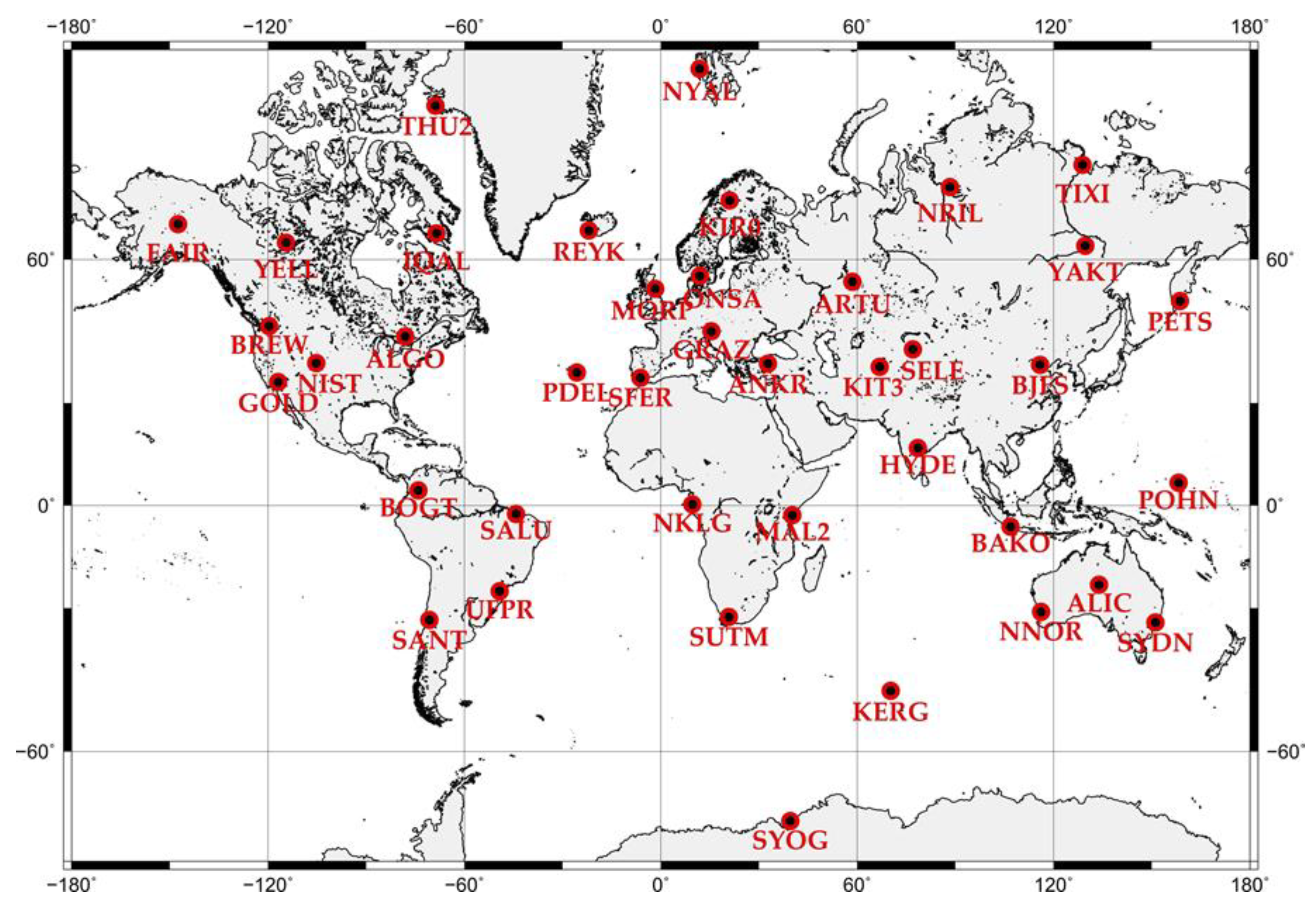
Forty homogenously distributed IGS points and their four-year solution time series provided by the Jet Propulsion Laboratory (JPL) for the period 2012 through 2016 were used (Figure 1). For this, we referred to the National Aeronautics and Space Administration (NASA)-JPL official website (http://sideshow.jpl.nasa.gov/post/series). Position time series for each IGS station concerning local topocentric coordinates north, east, and up (n, e, and u) and accompanying standard errors were downloaded.

First, the JPL continuous time series constituting daily position estimates were decimated into monthly sampled GPS campaign time series by picking only one position estimate (i.e., day fifteen here) from each month of the year. In practice, this means that the field operator occupies the geodetic survey point with a GPS receiver every month in a year. This might be considered an ideal survey procedure, which is much denser than the one measurement per year. Obviously this would be much more cumbersome than the traditional field work in which the geodetic mark is visited for a couple of consecutive days each year [1]. Considering this we worked on an alternative survey procedure in which the sampling is made selecting one position estimate (i.e., derived from full 24 h) every four months. This is surely superior to the sampling; one measurement per year with 8–10 h of observation session.

Secondly, we estimated the deformation rate from a four-year continuous JPL time series. Blewitt and Lavallee [17] and Wang, Turco, Soler, Kearns and Welch [25] assess the minimum span of continuous GPS time series for the appropriate determination of the deformation rate. They recommend a minimum span for deformation monitoring of between 2.5 and 4.5 years. Figure 2 shows GOLD continuous, monthly, and four-monthly decimated campaign time series.

Furthermore, to take into account the antenna set up error, we added some biases to the coordinate components north, east, and up. As noted earlier on, we generated synthetic GPS campaigns using the data of IGS continuously operating stations where the antennas are usually on top of concrete pillars and their position does not change over time. However, campaign GPS measurements are usually collected by mounting the GPS antenna on top of a tripod while visiting the survey sites. This would create an error due to possible improper centering and incorrect measurement of the antenna height. Considering the antenna set up error would be randomly distributed over a long time period, it was generated synthetically as a random noise produced from a MATLAB routine. On the magnitude of the bias we referred to Dixon [26] and Gili, Corominas and Rius [27] who assesses the antenna set-up errors. The bias is noted to be 1–3 mm from the setup of tripod mounted GPS antennas using optical plummets. Therefore we generated white noise with the standard deviation of 3 mm. The best way to assess this would be taking campaign measurements near to (<10 m) continuous stations however we would not be able to produce our results globally.

3. Velocity Estimation Using Least Squares Analysis and Statistical Testing

Annual and semi-annual components were included in the least squares estimation as the time dependent coefficients, and the unknown parameters a, b, c₁, c₂, d₁, d₂, and x_off were estimated using the regression equation:

$$\mathrm{y}\left(\mathrm{t}\right)=\mathrm{a}+\mathrm{b}.\mathrm{t}+{\mathrm{c}}_1.\sin \left(\frac{2\pi t}{T_1}\right)+{\mathrm{d}}_1.\cos \left(\frac{2\pi t}{T_1}\right)+{\mathrm{c}}_2.\sin \left(\frac{2\mathsf{\pi }\mathrm{t}}{T_2}\right)+{\mathrm{d}}_2.\cos \left(\frac{2\pi t}{T_2}\right)+o.x_{off}+v\left(t\right)$$

(1)

where a is the intercept, b is the velocity, c₁ and d₁ are periodical constituents for the annual term whereas c₂ and d₂ are periodical constituents for the semi-annual term. In addition, T₁ and T₂ are periods of annual and semi-annual periodic components, which were taken to be 1.0 cycle and 0.5 cycles, respectively. x_off is an offset term and v(t) represents residuals. Bogusz and Klos [20] performed a detailed study on the IGS continuous time series, where a wide spectrum of periodic components were investigated. However, here only the major annual and semi-annual periodicities of the seasonal variation were included in the Least Squares Estimation (LSE) analysis for simplicity. Similarly, we did not choose our stations from places in which the time series contain transients. This would have requested detailed modeling and station specific care. The reader should refer to Ji and Herring [28,29] for transients in time series.

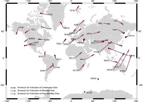
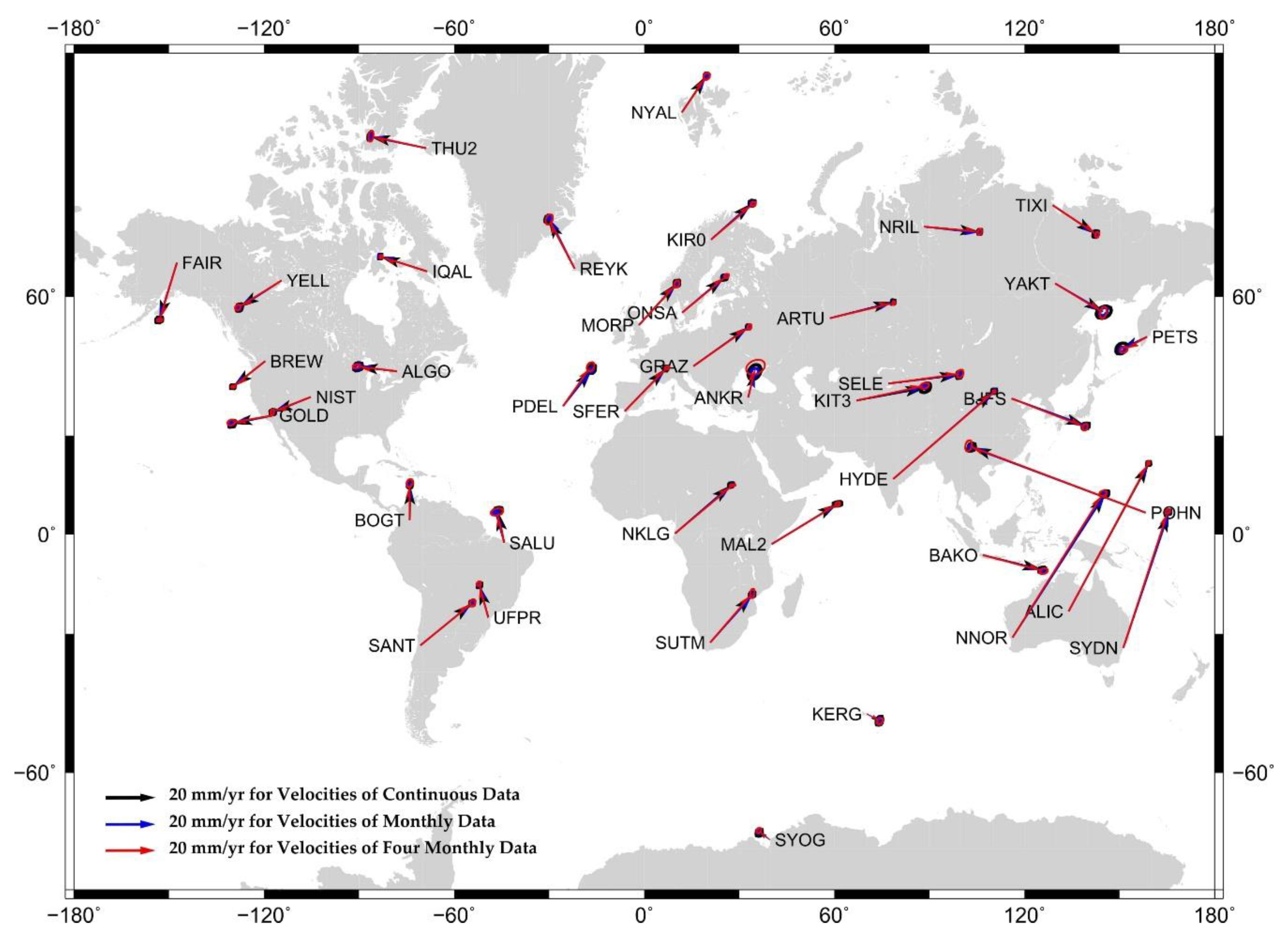
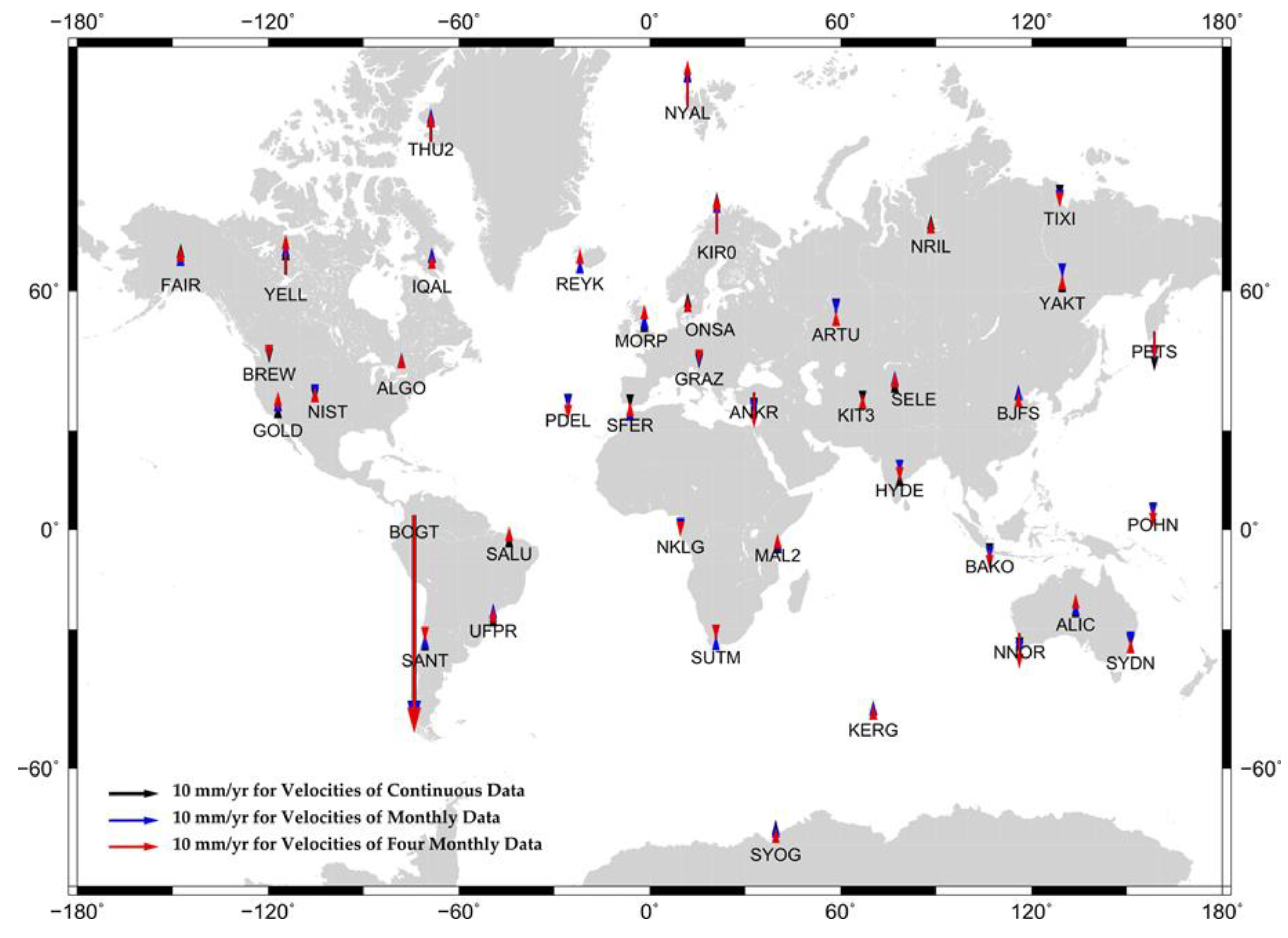
The velocity b in Equation (1) was estimated for all; monthly, four-monthly, and continuous data. Figure 3 and Figure 4 show the horizontal and vertical velocity fields of continuous and monthly sampled data.

In addition, the other unknown parameters and their associated standard errors were also computed for n, e, and u components. Then we applied a Student’s t-test as to whether the velocities from the monthly (or four-monthly) solutions differ significantly from those of the daily solutions. The formulation and the notation for the t-test from a multi-regression analysis is given in

Table 1. Notation and formulation for the Student’s t-test from multi-regression analysis.

Test Statistic	Critical Region
$T=\frac{{\mathrm{b}}_{\mathrm{m}}-{\mathrm{b}}_{\mathrm{d}}}{\mathrm{s}.\sqrt{{\mathrm{q}}_{\mathrm{i}}{\mathrm{q}}_{\mathrm{i}}}}$	$T\langle -1.96\mathrm{or}\mathrm{T}\rangle 1.96$

b_d = daily velocity; b_m = monthly (or four-monthly) velocity; s = unit variance from LSE; q_i = element of the cofactor matrix.

.

The zero hypothesis was set to be H₀: b_m = b_d and the alternative hypothesis H_A: b_m ≠ b_d. If, for a two-sided test, T exceeds ±1.96 with α = 0.05 then H₀ is rejected. In other words, the velocity estimated from monthly (or four-monthly) GPS campaigns is significantly different than that of the continuous GPS.

In the Figure 3 and Figure 4, antenna set-up errors were not yet imposed on the velocities. Obviously the estimated deformation rate could be biased due to this. Horizontal velocities were given with error ellipses having a 95% confidence level. The ellipse unit was 10 mm in the figure. Note that velocities from the continuous, monthly, and four-monthly time series were pretty much comparable (i.e., the direction and magnitude of black, blue, and red arrows coincided well). 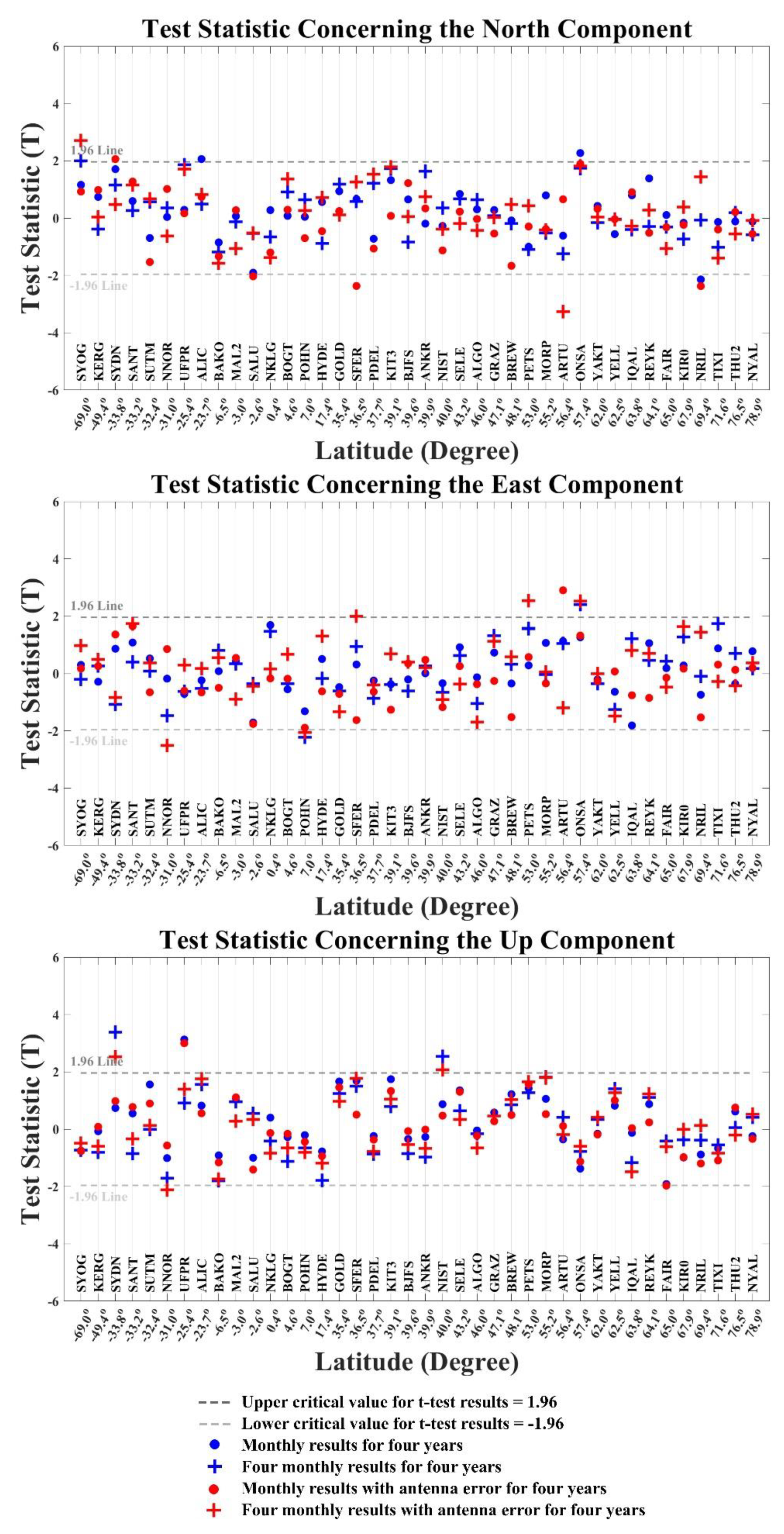The detailed results of the statistical hypothesis testing, which are not obvious in Figure 3 and Figure 4 are given in Figure 5. It is seen from the figure that a tremendous amount of success was gained over the study of Akarsu, Sanli and Arslan [22] and Duman and Sanli [23]. First of all, the effect of antenna set-up errors were clearly seen on all three components (c.f. the majority of red solid circles and plus signs over the blue ones). Velocity estimation was further degraded when antenna set up errors were introduced to GPS baseline components. Secondly, the success rate of the vertical component showed about 85% improvement over the study of Duman and Sanli [23].

Extending the observation session from 8–10 h to 24 h significantly improved the vertical deformation rates estimated. The velocity estimation for the north and east components was also improved by about 25–40%. Comparisons can also be made between monthly and four-monthly results. Antenna set-up biased results of four-monthly solutions gave about 8% coarser results than the antenna set-up biased one-monthly results.

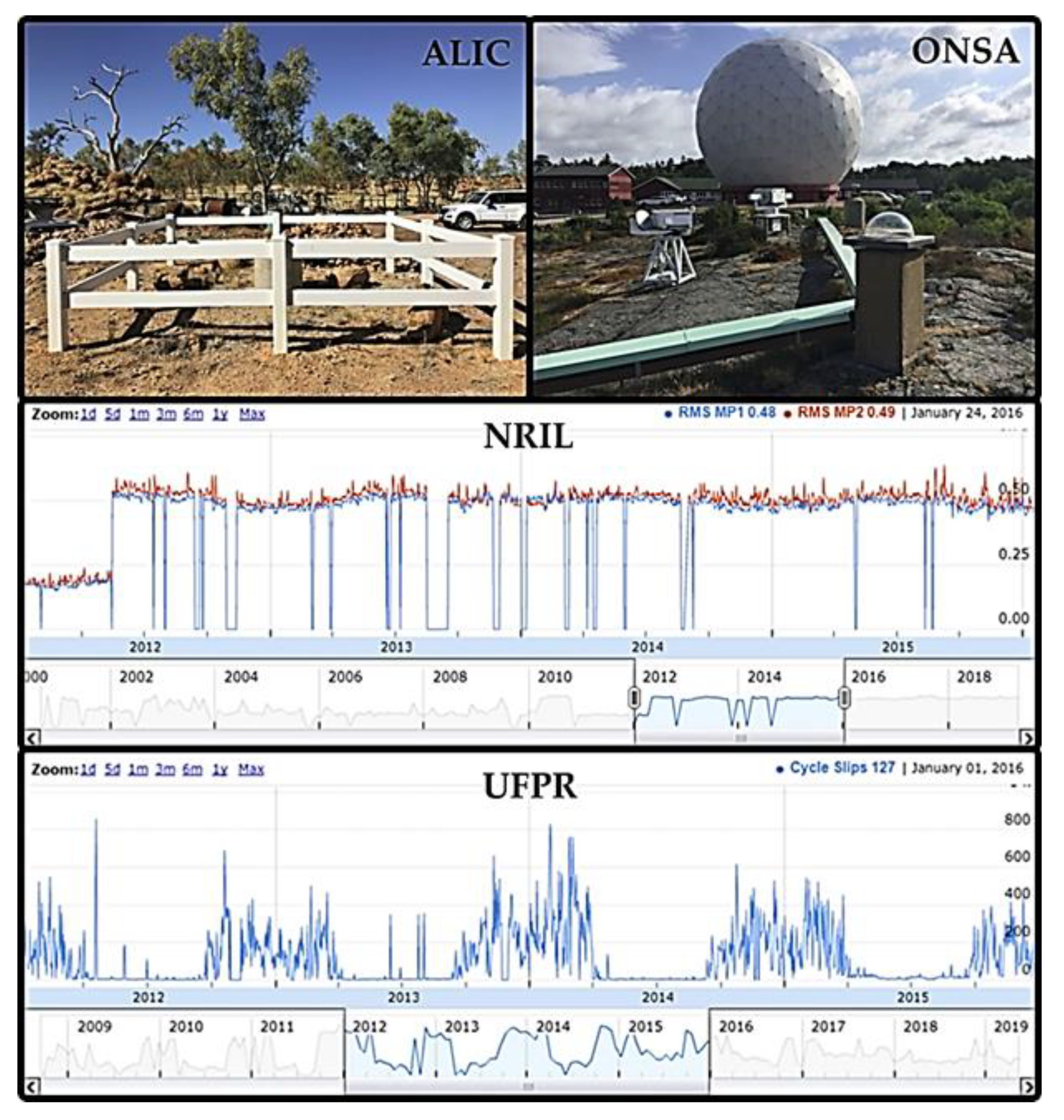
One other detail that we noticed in Figure 5 was that the north component had three blue solid circles, which means some of the estimated velocities significantly differed from the truth without taking into consideration antenna set-up errors. These were the stations ALIC, ONSA, and NRIL. The same applies to the up component in that the velocity estimated at the station UFPR significantly differed from the truth. At this stage, we referred to the site specific information released by the IGS (Figure 6) and some geological reports to interpret this unexpected positioning differences. The top left figure illustrates the environment of the station ALIC. The station was installed on a bedrock, which is the standard for monitoring the tectonic motion. Multipath level and cycle slip level were very low. However it is noted in the figure that the station was surrounded by trees. The fact that the velocity estimated at ALIC significantly differed from the truth might be ascribed to signal attenuation due to tree leaves, and this deteriorates the positioning [30].

The top right figure of Figure 6 gives the environment of ONSA. ONSA was established on a bedrock. However it was placed at a space laboratory in which data were collected from other geodetic instrumentation such as VLBI antennas, gravimeter, and tide-gauges. Note the radome of a huge radio-telescope behind the GPS antenna in the figure. The reason that the estimated velocity at this station significantly differed from the truth might be ascribed to the multipath environment at the vicinity of the GNSS antenna given MP1 and MP2 multipath levels were about 0.80 for the station. In the log file of the station was reported various events in regard to the low data quality, multipath reduction, and equipment repairs between the years 2012 and 2016, which corresponds to our data analysis period here.

In the middle part of Figure 6 is represented the multipath quality of the station NRIL. NRIL was located on top of the roof of the seismology building as stated in the log file released by the IGS. Bukchin, et al. [31] states the station is in a tectonically stable place. The tectonic interaction between Pamir and Tien Shan was examined taking NRIL as one of the stable Eurasian reference stations in the GNSS analysis [32]. However, the multipath environment on the roof as well as shaking of the building might have degraded the positioning quality, given MP1 0.48 and MP2 0.49 multipath levels were comparatively higher. Unfortunately, a picture giving the site description of the GNSS station NRIL was not available on the internet.

Salamuni, et al. [33] states that the place where UFPR was installed is in a tectonically active region. Erosions and normal faulting are encountered in the region. Furthermore, a tremendous number of cycle slips occurred during the data collection period 2012 through 2016. See the bottom part of Figure 6 for this. High tectonic and cycle slipping activity might have caused the deterioration in the vertical positioning quality of UFPR.

4. Conclusions

From a global network of IGS stations, we carried out an experiment in which the ground deformation rate (i.e., velocity) due to tectonic motion estimated from campaign measurements was compared with the ground deformation rate obtained from continuous GPS data. Continuous GPS time series constructed for the IGS stations by NASA JPL were utilized in the analysis. Campaign GPS time series were generated by decimating the four-year continuous positioning solutions into monthly and four monthly samples. Learning lessons from the success of GPS campaigns performed with 8–12 h in the literature, we extended the duration of measurements to a full 24 h. In other words, synthetic campaigns from continuous data were generated using solutions from 24 h data. Previously it was found that determining tectonic motion from a traditional 8–12 h GPS campaigns was not comparable to the one produced from GPS campaigns using 24h data. With a careful refinement procedure, on the average only 50–70% of the velocities estimated for horizontal components were usable. Only 10% of the velocities produced from the vertical component of 8–12 h campaigns was comparable to the one produced from 24 h campaigns. These assessments were produced with 95% confidence level and considering a full 15-year time series. Here, we synthetically applied two different sampling from the continuous data; one measurement per month and one measurement per four months. Considering practical concerns we used four-year time series, which is a minimum data requirement for reliable deformation monitoring.

In addition, in this phase of the work, we took into account antenna tripod set up errors on positioning. Note that the data sampled from continuous IGS stations neglected the antenna set up errors. Referring to the literature for the magnitude of the antenna error, GPS campaign measurements were synthetically biased. As expected, in general, the deformation rate obtained from GPS campaigns performed once per month agreed better with the deformation rate produced from continuous GPS. However, repeating GPS campaigns once every month would be cumbersome to many operators in the field. Here, the success of horizontal positioning accuracy by campaign measurements using observations once every four months had been improved by about 25–40% whilst the success of the vertical positioning had been improved by about 85% compared to previous studies. Extending the observation duration from 8 h to 24 h played the key role in gaining this.

Note that the assessments made here were only for the determination of tectonic motion. The 1-sigma velocity estimation error of the campaign data was a factor of 5–10 coarser than those of the continuous data. The conclusions made here obviously would not apply to the monitoring of, say a fault creep requiring much more attention. For the assessment of GNSS stations in tectonically active regions, the reader should refer to site specific reports of the IGS and geological assessment of the region for better interpretations. Our overall conclusion is that the field operator is now very near to the 95% confidence level in monitoring of the tectonic motion especially for the north and up components if the observation session is extended to 24 h and campaigns are repeated every four months.