Abstract
Haze removal is a pre-processing step that operates on at-sensor radiance data prior to the physically based image correction step to enhance hazy imagery visually. Most current haze removal methods focus on point-to-point operations and utilize information in the spectral domain, without taking consideration of the multi-scale spatial information of haze. In this paper, we propose a multi-scale residual convolutional neural network (MRCNN) for haze removal of remote sensing images. MRCNN utilizes 3D convolutional kernels to extract spatial–spectral correlation information and abstract features from surrounding neighborhoods for haze transmission estimation. It takes advantage of dilated convolution to aggregate multi-scale contextual information for the purpose of improving its prediction accuracy. Meanwhile, residual learning is utilized to avoid the loss of weak information while deepening the network. Our experiments indicate that MRCNN performs accurately, achieving an extremely low validation error and testing error. The haze removal results of several scenes of Landsat 8 Operational Land Imager (OLI) data show that the visibility of the dehazed images is significantly improved, and the color of recovered surface is consistent with the actual scene. Quantitative analysis proves that the dehazed results of MRCNN are superior to the traditional methods and other networks. Additionally, a comparison to haze-free data illustrates the spectral consistency after haze removal and reveals the changes in the vegetation index.
1. Introduction
During the acquisition of optical satellite images, light reflected from the surface is usually scattered in the process of propagation due to the presence of water vapor, ice, fog, sand, dust, smoke, or other small particles in the atmosphere. This process reduces the image contrast and blurs the surface colors, leading to difficulties in many fields including cartography and web mapping, land use planning, archaeology, and environmental studies. Therefore, an effective haze removal method is of great importance to improve the capability and accuracy of applications that use satellite images. Haze removal aims at eliminating haze effects on at-sensor radiance data prior to the physically based image correction that converts at-sensor radiance to surface reflectance. In cloudy areas, there is no information about the ground surface, whereas in areas affected by haze the image still contains valuable spectral information. Although haze transparency presents an opportunity for image restoration, an efficient and widely applicable haze removal method for handling various haze or thin clouds is still a great challenge, especially when only a single hazy image is available.
Single-image based haze removal has made significant progress recently by relying on different assumptions and prior information. Chavez [1,2] presented an improved dark object subtraction (DOS) technique to correct optical data for atmospheric scattering, assuming a constant haze over the whole scene. Liang et al. [3,4] proposed a cluster matching technique for Landsat TM data, assuming that each land cover cluster has the same visible reflectance in both clear and hazy regions. The demand for existing aerosol transparent bands makes it impractical in some situations, as visible and near-infrared bands are usually contaminated by haze. Zhang et al. [5] proposed a haze optimized transformation (HOT) to characterize the spatial distribution of haze based on the assumption that the radiances of the red and blue band are highly correlated for pixels within the clearest portions of a scene and that this relationship holds for all surface types. However, the sensitivity of HOT to water bodies, snow cover, bare soil, and urban targets limits its application. To reduce the impact of spurious HOT responses, various strategies are proposed in the literature [6,7,8,9]. Liu et al. [10] developed a background suppressed haze thickness index (BSHTI) to estimate the relative haze thickness and used a virtual cloud point method to remove haze. Makarau et al. [11,12] utilized a haze thickness map (HTM) for haze evaluation, based on the premise that a local dark object reflects the haze thickness of the image. Shen et al. [13] developed a simple and effective method by using a homomorphic filter [14] for the removal of thin clouds in visible remote sensing (RS) images.
He et al. [15] discovered the dark channel prior (DCP) that in most of the non-sky patches of haze-free outdoor images, at least one color channel has very low intensity at some pixels. DCP combined with an image degradation model has proved to be simple and effective enough for haze removal. However, it is computationally intensive and may be invalid in special cases. Some improved algorithms [16,17,18,19,20] are proposed to overcome these limitations. The great success of DCP in computer vision attracted the attention of researchers working on satellite application. Long et al. [21] redefined the transmission of DCP and used a low-pass Gaussian filter to refine the atmospheric veil instead of using soft matting method. Pan et al. [22] noted that the average intensity of remote sensing images’ dark channel is low, but not close to zero. Thus, they added a constant term into the image degradation model for haze removal. Jiang et al. [23] utilized a proportional strategy to gain accurate haze thickness maps for all bands from the original dark channel in order to prevent underestimation. These methods succeed in solving specific scenarios in practical applications. However, adjustable parameters in an algorithm must be well designed for various situations to obtain ideal results, which requires a considerable number of experiments on a wide variety of selected images. In addition, these algorithms are effective for local operations, but cannot handle a whole satellite image properly.
In recent years, haze removal methods were developed in the machine learning framework. Tang et al. [24] combined four types of haze-relevant features with random forests [25] to estimate the haze transmission. Zhu et al. [26] created a linear model to evaluate the scene depth of a hazy image, depending on a prior color attenuation. The parameters of the model are learned with a supervised learning method. Despite the remarkable progress, the limitation of these methods lies in the fact that the haze-relevant features or heuristic cues are not effective enough. Following the success of the convolutional neural network (CNN) for image restoration or reconstruction [27,28,29], Cai et al. [30] proposed DehazeNet, a trainable CNN-based end-to-end system for haze transmission estimation. DehazeNet provides superior performance on natural images over existing methods and maintains efficiency and ease of use. Nevertheless, the “shallow” DehazeNet cannot handle RS images properly due to the dramatic spatial variability of images or haze in it and complicated nonlinear relationship between haze transmission and spectral-spatial information of images [31]. It is believed that deep learning architectures are generally more robust to the nonlinear input data owing to the ability to extract high-level, hierarchical, and abstract features. In the RS community, large numbers of deep networks are currently developed in the field of hyperspectral image classification [32,33], semantic labelling [34,35], image segmentation [36], object detection [37,38], change detection [39], etc. However, to the best of our knowledge, a deep network has not been proposed for haze removal of RS images.
In this study, we propose a multi-scale residual convolutional neural network (MRCNN) for the first time that can learn the mapping relations between hazy images and their associated haze transmission automatically. MRCNN behaves well in predicting accurate haze transmission by extracting spatial–spectral correlation information and high-level abstract features from hazy image blocks. Specifically, the dilated convolution is utilized to obtain local-to-global contexts including details of haze and the trend of haze spatial variations. Technically, residual blocks are introduced into the network to avoid loss of weak information, and dropout is used to improve the generalization ability and prevent overfitting. Experiments on Landsat 8 Operational Land Imager (OLI) data demonstrate the effectiveness of MRCNN for haze removal.
The remaining parts of this paper are organized as follows. Section 2 briefly introduces the haze degradation model and provides some basic information about CNNs. Section 3 describes the details of the proposed MRCNN. The experimental results and comparison to other state-of-the-art methods are showed in Section 4. The model performance, spectral consistency before and after haze removal, and influence on vegetation index are discussed in Section 5. Finally, our conclusions are outlined in Section 6.
2. Preliminaries
2.1. Haze Degradation Model
To describe the formation of a hazy image, different haze models have been proposed in the literature. The widely used models include an additive model [11,12] and a haze degradation model [40,41]. Herein, we adopt the latter for the sake of developing a trainable end-to-end deep neural network. The mathematical expression is written as follows [40,41]:
where is the position of a pixel in the image, is the hazy image, is the clear image to be recovered, is the global atmospheric light, represents the haze transmission describing the portion of atmospheric light that reaches the sensor, is the distance between the object and the observer, and represents the scattering coefficient of the atmosphere. The clear image can be recovered after and are estimated properly. Equation (2) suggests that when goes to infinity, approaches zero. Together with Equation (1) we have:
In a practical imaging process, cannot be infinity, but it can be a long distance that leads to a very low transmission . Thus, the atmospheric light is estimated as follows:
The discussion above indicates that to recover a clear image, i.e., to achieve haze removal, the key is to estimate an accurate haze transmission map. In this paper, we plan to build a deep neural network for the estimation of haze transmission according to the input of hazy images, i.e., taking hazy images as input and outputting corresponding transmission maps. Once and are estimated, the clear image can be recovered as follows:
In this paper, the haze degradation model is used to simulate training pairs of hazy patches and target haze transmission from sampled clear blocks, and finally recover a clear image according to the predicted transmission map.
2.2. CNNs
CNNs [42] are biologically inspired variants of multilayer perceptron that can learn hierarchical representations from raw data and are capable of initially abstracting simple concepts and then constructing more complex concepts by comprehending the simpler ones. There are two special aspects in the architecture of CNN, i.e., sparse connections and shared weights. CNNs exploit a spatially local correction by enforcing a local connectivity pattern between neurons of adjacent layers. We illustrate this graphically in Figure 1, where units in layer m are connected to three spatially contiguous units in layer m − 1. In addition, in CNNs, each convolutional filter is replicated across the entire layer, sharing the same weights and biases. In Figure 2, the weights of the same color are shared-constrained to be identical. In this way, CNNs are able to achieve better generalization on vision problems and the learning efficiency is increased by greatly reducing the number of free parameters to be learnt.
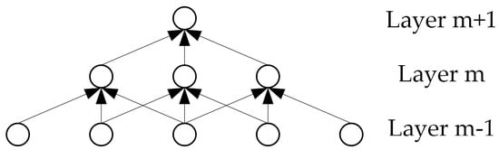
Figure 1.
Local connectivity pattern in CNNs. Each unit is connected to three spatially contiguous units in the layer below.
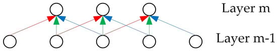
Figure 2.
Shared weights in CNNs. The same color indicates the same weight.
The input and output of each layer are sets of arrays called feature maps. A standard CNN usually contains three kinds of basic layers: a convolutional layer, nonlinear layer, and pooling layer. Deep CNNs are constructed by stacking several basic layers to form the deep architecture.
The convolutional layer performs a series of convolutional operations on the previous layer with a small kernel (e.g., 3 × 3, 5 × 5, etc.). Each convolutional operation computes the dot product between the weights of the kernel and a local region (called the receptive field) of the input feature map. The value at position (x, y) of the jth feature map in the mth layer is denoted as follows:
where i indexes the feature map in the (m − 1)th layer connected to the current jth feature map, represents the number of feature maps in (m − 1)th layer, is the weight at position (p, q) connected to the ith feature map, and are the height and the width of the convolutional kernel, and is the bias of the jth feature map in the mth layer. Figure 3 shows two layers of a CNN. Layer m − 1 contains four feature maps and layer m contains two feature maps. The pixels in layer m (blue or red squares) are computed from the pixels of layer m − 1, which fall within their 2 × 2 receptive field in the layer below (shown as colored rectangles). It is noted that the subscript m is omitted in the weight matrices.
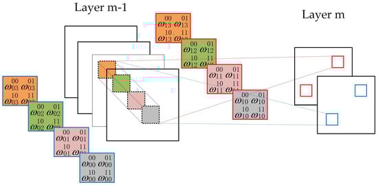
Figure 3.
Example of a convolutional layer. Pixels in layer m (blue or red squares) are computed from pixels of layer m − 1 that fall within their 2 × 2 receptive field in the layer below (shown as colored rectangles). Weight matrices for feature maps in layer m are listed in the squares with the same color.
The nonlinear layer embeds a nonlinear activation function that is applied to each feature map to learn nonlinear representations. The rectified linear unit (ReLU) [43,44] is widely used in recent deep neural networks and can be defined as . In other words, ReLU thresholds the non-positive value as zero and keeps the positive value unchanged. ReLU can alleviate the vanishing gradient problems [45] and speed up the learning process to achieve a considerable reduction in training time [46].
The pooling layer provides a way to perform sub-sampling along the spatial dimension and to make features invariant from the location. It summarizes the outputs of neighboring groups of neurons in the same kernel map. There are two kinds of pooling operations: max-pooling and average-pooling. The former samples the maximum in the region to be pooled while the latter computes the mean value. Figure 4 shows an example of different pooling operations. Traditionally, neighborhoods summarized by adjacent pooling units do not overlap. Overlapping max-pooling (OMP) is used in ImageNet [46], which is proven to be an effective way to avoid overfitting.
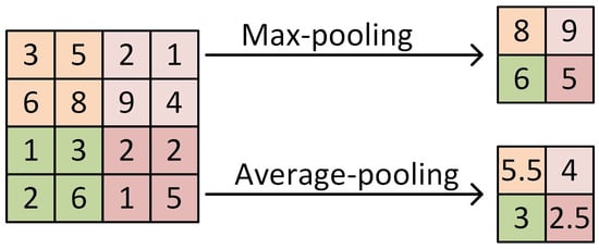
Figure 4.
Example of pooling operations. The kernel size is 2 × 2 and the stride is 2 pixels.
3. Data and Method
3.1. Data
The remote sensing (RS) images used in this study are Landsat 8 Operational Land Image (OLI) data, obtained from the Earth Explorer of the United States Geological Survey (USGS) (https://earthexplorer.usgs.gov/). The OLI is an instrument onboard the Landsat 8 satellite, which was launched in February 2013. The satellite collects images of the Earth with a 16-day repeat cycle. The approximate scene size is 170 km north–south by 183 km east–west. In total, the OLI sensor has eight multispectral bands. The spatial resolution of the OLI multispectral bands is 30 m, and the digital numbers (DNs) of the sensor data are 16-bit pixel values. As haze usually has an influence on the visible and near-infrared (NIR) bands, sequentially including band 1 (coastal/aerosol, 0.43–0.45 μm), band 2 (blue, 0.45–0.51 μm), band 3 (green, 0.53–0.59 μm), band 4 (red, 0.64–0.67 μm), and band 5 (NIR, 0.85–0.88 μm), thus just the first five bands of the OLI images are used as inputs of the following network for the prediction of haze transmission.
3.2. CNN Architecture
The haze degradation model in Section 2.1 suggests that the estimation of the haze transmission map is of the most important task to recover a clear image. To this end, we present a multi-scale residual CNN (MRCNN) to learn the mapping relations between the raw hazy images and their associated haze transmission automatically. Figure 5 illustrates the architecture of MRCNN, which mainly consists of four modules: spectral–spatial feature extraction, multi-scale context aggregation, residual learning and fully connected layers. The detailed configurations of all layers are summarized in Table 1, and are explained in the following.
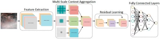
Figure 5.
Overview of the proposed MRCNN. The network mainly consists of four modules: spectral–spatial feature extraction, multi-scale context aggregation, residual learning, and fully connected layers.

Table 1.
Detailed configurations of MRCNN. Conv represents the convolutional layer, Conv-i (i = 1, 2, 4) represents the dilated convolutional layer, whose dilation rate equals i, OMP represents the overlapping max-pooling layer, and FC represents the fully-connected layer.
3.2.1. Spectral–Spatial Feature Extraction
To address the ill-posed nature of the single image dehazing problem, existing methods propose various empirical assumptions or prior knowledge to extract intermediate haze-relevant features, such as dark channel [15], hue disparity [47], and color attenuation [26]. These features reflect different perspectives of the original image and are helpful for the estimation of haze transmission. Inspired by this, we design the first module of (M1) MRCNN for haze-relevant feature extraction. In the field of image classification, it is proved that the usage of spectral features and spatial information in combined fashion can significantly improve the final accuracy [48]. Thus, we utilize 3D convolutional kernels to extract spectral and spatial features simultaneously in M1. The 3D convolution operation computes each pixel in association with d × d spatial neighborhoods and n spectral bands to exploit the important discriminative information and take full advantage of the structural characteristics of the 3D input data cubes.
After feature extraction, we apply a Maxout unit [49] for nonlinear mapping as well as dimension reduction, which is able to eliminate information redundancies and improve the performance of the network by removing multi-collinearity. Maxout generates a new feature map by taking a pixel-wise maximization operation over k feature maps in the layer below:
where j indexes the feature map in the mth layer, i indexes the feature map in the (m − 1)th layer, means the number of feature maps in mth layer, and denotes multiplicative operation.
Specifically, M1 connects to the input layer that contains 3D hazy patches of size 5 × 16 × 16 (channels × width × height, similarly hereafter). The inputs are padded with one pixel in the spatial dimensions. We use zero padding in this paper. The convolutional layer filters inputs with 64 kernels of size 5 × 3 × 3. The stride of these kernels, or the distance between the receptive fields’ centers of the neighboring neurons, is one pixel. The 3 × 3 convolutional filter is the smallest kernel to seize patterns in different directions, such as center, up/down, and left/right. Additionally, small convolutional filters will increase the nonlinearities inside the network and thus make the network more discriminative. The Maxout unit takes four feature maps that are generated by the convolutional layer in a non-overlapping manner as input, calculates maximum value at each pixel, and finally outputs one feature map with an unchanged size. Finally, M1 outputs 16 feature maps of size 16 × 16.
3.2.2. Multi-Scale Context Aggregation
When observing an image, we often zoom in or out to recognize its characteristics from local to global. This process demonstrates that features in different scales are important for inference of relative haze thickness from a single image when additional information is lacking. Herein, we design the second module (M2) for multi-scale context aggregation. Basically, there are two approaches to gain the feature in a large receptive field: deepening the network or enlarging the size of the convolutional kernels. Although theoretically, features from high-level layers of a network have a larger receptive field on the input image, in practice, they are much smaller [37]. Enlarging the convolution kernel size directly can also obtain wider information, but it is always associated with exponential growth of learnable parameters. Dilated convolution [50] provides us with a new approach to capture multi-scale context by using different dilation rates. Dilated convolution expands the receptive field without extra parameters so that it can efficiently learn more extensive, powerful and abstract information. In addition, dilated convolution is capable of aggregating multi-scale contextual information without losing resolution or analyzing rescaled images.
Figure 6 illustrates an example of 2-dilated convolution. The convolution kernel is of size 3 × 3 and its dilation rate equals 2. Thus, each element in the feature map after dilated convolution has a receptive field of 7 × 7. In general, the size of receptive field of 3 × 3 filters with different dilation rate can be computed as follows:
where represents the set of natural numbers. To make the size of resulting feature map unchanged, the padding rate should be set as in the corresponding direction. By setting a group of small-to-large dilation rates, a series of feature maps with local-to-global contexts can be obtained. Local contexts record low-level details of haze while global contexts identify the trend of haze spatial variations with its wide visual cues. Meanwhile, generated feature maps with multi-scale contexts can be aligned automatically due to their equal resolution.
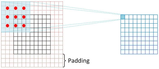
Figure 6.
An illustration of dilated convolution. The input feature map is of size 9 × 9 and padded with 3 pixels. The padding value is zero. The convolution kernel is of size 3 × 3 and its dilation rate equals 2. Each element in the resulting feature map has a receptive field of 7 × 7.
Specifically, M2 takes as input the output of M1. It contains three parallel sub-layers using 1-dilated, 2-dilated and 4-dialated convolution, respectively. Each layer has 16 convolution kernels of size 3 × 3. Thus, their actual receptive fields correspond to 3 × 3, 7 × 7 and 15 × 15. To ensure the multi-scale outputs are with the same size, inputs for three sub-layers are padded with 1, 3 and 7 pixels, respectively. Multi-scale feature maps are concatenated to form a 48 × 16 × 16 feature block before being fed into the following OMP layer. The kernel size of the pooling layer is 9 × 9 and its stride is 1 pixel. Therefore, the final output of M2 is 48 feature maps of size 8 × 8.
It should be noted that no activation function is used in M1 and M2 due to the experimental fact that remote sensing image blocks usually produce large gradients in the early stage. A large gradient flowing through a ReLU neuron could cause the weights to update in such a way that the neuron will never activate on any data point again. If this occurs, then the gradient flowing through the unit will forever be zero from that point on, i.e., the training process would “die”. As the process of extracting features proceeds, the distribution of the feature maps in deeper layers tends to be more stable. Therefore, it is more appropriate to add the ReLU activation function in the deeper convolutional layers instead of the shallow ones.
3.2.3. Residual Learning
Obtaining an accurate estimation of haze is not easily accessible, because surface coverage, not haze, is the dominant information in RS images. The features from high-level layers are likely to lose weak information, such as haze. Deeper networks also face a degradation problem [51]: with an increase in the network depth, accuracy gets saturated and then degrades rapidly; this outcome is not caused by overfitting. Herein, we introduce residual learning [52] to resolve these issues. Instead of anticipating that each layer will directly fit a desired underlying mapping, we explicitly allow some layers to fit a residual mapping. Formally, denoting the desired underlying mapping as , we expect stacked layers to fit another mapping of . Therefore, the original mapping is recast into . The residual learning is very effective in deep network, because it is easier to fit than to directly fit when the network deepens.
Figure 7 shows the residual block used in the third module (M3). All three convolutional layers have k kernels of size 3 × 3, equipped with ReLU nonlinear activation function. The first convolutional layer outputs its learned features , which are sent to the second and third convolutional layer for learning residual features . and are then fused using the sum operation to form the target features . The following OMP layer performs local aggregation on without padding. Specifically, M3 connects to the outputs of M2, which are of size 48 × 8 × 8. The inputs are sent to two sequential residual blocks. The convolutional layer in the first block has 64 kernels while 128 kernels are used in the second block. The kernel size of the OMP layers is 5 × 5 and 3 × 3, respectively. Finally, M3 outputs features of size 128 × 2 × 2.
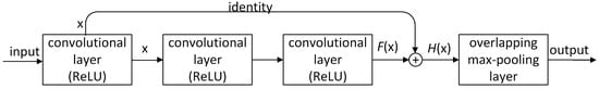
Figure 7.
Residual block used in MRCNN. The first convolutional layer outputs its learned features x, which are sent to the second and third convolutional layer for learning residual features F(x). F(x) and x are then fused using a sum operation to form the target features H(x).
3.2.4. Fully Connected Layers
At the end of the proposed network, we utilize fully connected (FC) layers to achieve our regressive task, i.e., predicting haze transmission relying on abstract features from stacked convolutional layers. The feature maps of the last convolutional layer are flattened and fed into the FC layers. However, the FC layers are prone to overfitting, thus hampering the generalization ability of the overall network. Dropout, a regularization method proposed by Hinton et al. [53], randomly sets a portion of the hidden neurons to zero during training. The dropped neurons do not contribute in the forward pass and are not used in the back-propagation procedure. Dropout has been proven to improve the generalization ability and largely prevents overfitting [54].
Specifically, three FC layers are implemented with 512, 64, and one nodes, respectively. They computes their output as , where are weight matrices, are bias vectors, is the output of the previous layer and represents the ReLU activation function. In addition, we have allowed a 50% dropout in the first FC layer. Finally, the FC layers produce a single value representing the haze transmission at the central pixel of each input of hazy patches.
3.3. Training Process
To train the designed MRCNN, a large number of training samples consisting of hazy patches and their corresponding haze transmissions are required. However, it is challenging to obtain the real haze transmission. Inspired by Tang et al.’s method [24], we generate training samples from clear image blocks by simulating the haze degradation process according to the model in Section 2.1. This work is based on two assumptions: first, the image content is independent of transmission, i.e., the same content can appear under any transmission; and second, the transmission is locally constant, i.e., image pixels in a small patch have a similar transmission. Given a clear patch , the atmospheric light , and a random transmission , a simulated hazy patch is generated as . As the surface radiances reached the sensor would be too weak when the transmission is lower than 0.3, we restrict in the range . To reduce the uncertainty of variables in learning, is simply set to 1 in all five channels, i.e., . Herein, a training pair is composed of the generated and given .
Considering the difficulty of building a complete dataset containing various kinds of surface cover types, clear samples are collected in a local clear region of a single scene of Landsat 8 OLI data (path 123, row 032, acquisition date 23 September 2015) in our experiments. In addition, if too many surface types are selected for training, the dataset would become extremely large when ensuring sufficient samples for each type, which requires a considerable amount of computer memory and training time. In total, 60 clear blocks of size 240 × 240 are sampled from the test scene. Some examples are shown in Figure 8. All original clear blocks are normalized using the max-min method to ensure identical scale and that the atmospheric light equals 1. For each block, we uniformly generate 20 random transmissions to generate hazy blocks, which are then tiled into patches with a size of 16 × 16. Thus, 270,000 simulated hazy patches are collected. To ensure the robustness, these patches are shuffled to break potential correlation. Finally, all patches are sorted into a 90% training set and a 10% testing set, whose numbers are 243,000 and 27,000, respectively. Hereafter, we refer to this dataset as D1. It is important to note that the simulated patches are directly used as input of the training network without additional normalization, which would change the real haze depth.
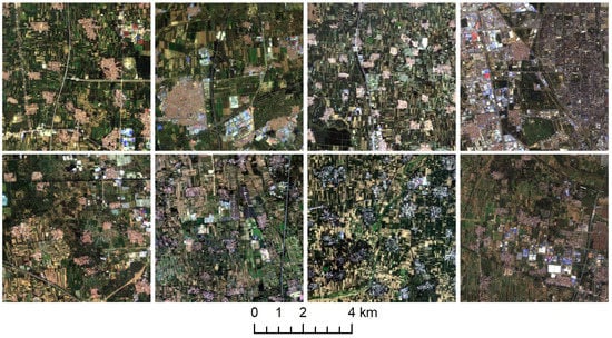
Figure 8.
Examples of clear blocks sampled from Landsat 8 OLI data (path: 123, row: 32, acquired date: 23 September 2015).
The MRCNN is trained through mini-batch stochastic gradient descent (MSGD) and an early-stopping mechanism. Gradient descent is a simple algorithm in which we repeatedly make small steps downward on an error surface defined by a loss function of some parameters. MSGD estimates the gradient from a mini-batch of examples to proceed more quickly. The batch size is set to 500 in our training. As the predicted variable is continuous, we use the mean squared error as the loss function:
where refers to the real transmission value, represents the predicted value, and is the batch size. Early-stopping combats overfitting by monitoring the network’s performance on a validation set. This technique relinquishes on further optimization when the network’s performance ceases to improve sufficiently on the validation set, or even degrades with further optimization. During training, we randomly chose 80% of the training samples to learn the parameters and the remaining 20% of the training samples were used as the validation set to identify if the network was overfitting. In our experiments, if the validation score is not improved by 1.0 × 10⁻⁵ within 10 epochs, the training process is terminated. The testing set is used to assess the final prediction performance of the trained network with the best validation score. The filter weights of each convolutional layer are initialized through the Xavier initializer [45], which uniformly samples from a symmetric interval:
where is the number of input units, and is the number of output units. For the first convolutional layer, equals 45 (5 × 3 × 3) and equals 576 (64 × 3 × 3). The biases are set to 0. The learning rate is 0.01 and is decreased by 0.5 when reaching a learning plateau. We implement our model using the keras [55] package with the theano backend [56]. Based on the parameters above, the best validation score is 0.0289% obtained at epoch 198, with a test performance of 0.0288%. It takes 145.68 min to finish training using an NVIDIA Quadro K620 GPU. Hereafter, we refer to this trained MRCNN as MODEL-O.
3.4. Dehazing and Post-Processing
After finishing training, we can predict the haze transmission given a new hazy patch. It is feasible to feed a small block into the network at one time for prediction. For each pixel in the block, its 16 × 16 surrounding neighborhood is used for prediction of haze transmission. While for the pixels belonging to the borders of the block, a 16 × 16 surrounding neighborhood cannot be defined. We have implemented a simple algorithm to replicate borders that allows us to handle all the border pixels as any other pixel in the block, i.e., mirroring eight pixels, half of the patch size, of the border outwards, to create the corresponding patches of the original border pixels. When handling a full-size image that occupies considerable physical memory, it is necessary to slice the original image and mosaic the output tiles to avoid running out of computer memory. The adjacent tiles overlap each other with pixels whose number equals the size of training patch, i.e., 16 pixels in our test, to prevent visual disruption. Furthermore, the original hazy image should multiply a scale factor depending on the pixel depth of the original data to ensure that the input values are in [0, 1]. In this way, we can predict the complete haze transmission map of the input block or full-size image. Finally, the clear image can be recovered according to Equations (4) and (5). The lowest decile of predicted transmission map is used as the threshold in Equation (4).
Generally, the radiances of directed dehazing results are lower than that of the clear scenes, as both haze contribution and clear scene aerosol are removed entirely. Meanwhile, the inaccurate estimation of the atmospheric light might lead to potential residual of radiances. Herein, we utilize clear regions, least influenced by haze, as a reference for the compensation of scene aerosol or correction of the residual. We slice the predicted transmission map into tiles of size 200 × 200. The tile with the maximum mean is considered as the clear region. The aim of compensating is to ensure mean radiance of the dehazed block corresponding to the clear region equals to that of the original block in all bands. The process of compensation can be expressed as:
where is the band number, is the final radiance, is the directed recovered value, represents the mean value of the original clear image block, and represents the mean value of the directed recovered image block corresponding to the clear region.
3.5. Transferring Application
To reduce the demand for computer memory and time consumption, MODEL-O is trained on a limited dataset. It is feasible to apply MODEL-O for haze removal of surrounding areas that covers the similar surface types. When handling images in another region, a new trained network is required. Learning from the beginning usually costs too much and is unnecessary. Transfer learning is an effective approach to apply stored knowledge gained while solving one problem to a different but related problem. The core of haze removal in different areas is essentially the same, but the surface types are dissimilar. Thus, the new MRCNN can be retrained on the basis of MODEL-O.
We choose another scene (path 119, row 038; acquisition date 14 April 2013) to collect new training samples. In total, 40 blocks of size 240 × 240 are sampled and then 180,000 simulated hazy patches are generated for training. Hereafter, we refer to this dataset as D2. The filter weights and biases are initialized using the learned parameters of MODEL-O, and other settings remain unchanged. The best validation score is 0.0128% obtained at epoch 43, with a test performance of 0.0168%. It takes 31.32 min to complete the optimization. Herein, the retrained MRCNN is named MODEL-T.
After fine-tuning, MODEL-T gains the ability to handle images covering this new type of surface coverage and theoretically still owns the ability of the previous network. The trained network can extend its applicability constantly through transferring learning. The more new types of samples are used for fine-tuning, the stronger the network will be. We expect that the network will finally be capable of addressing various complex situations after several cycles.
4. Experimental Results
4.1. Dehazing Results on Simulated Images
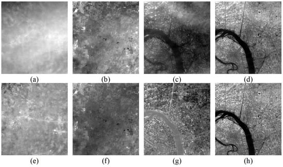
We first test the effectiveness of the trained networks using simulated hazy images. To better simulate the spatially varying haze, randomly generated haze transmissions are uniformly sampled in a small in range, such as [0.5, 0.6], [0.6, 0.8], etc., and smoothed with a Gaussian filter. The original clear images are used as references to assess the dehazed results quantitatively. MRCNN is compared with traditional haze removal methods (HOT [5], DCP [15], HTM [11]) and other networks (DehazeNet [30], VGGNet [57]). Herein, we use the trained networks with the best validation errors after 200-epoch training on D1 and 50-epoch fine-tuning on D2. Figure 9 shows an example of the dehazing results on simulated images using different methods. Serious color distortion appears in the HOT results. There still exists slight haze in DCP’s result. The colors in the HTM results are oversaturated. The recovered image of DehazeNet looks dim and has poor local contrast. In contrast, the results of VGGNet and MRCNN are better visually.
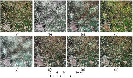
Figure 9.
Dehazing results of different methods on simulated images: (a) original clear image; (b) HOT [5]; (c) DCP [15]; (d) HTM [11]; (e) simulated hazy image; (f) DehazeNet [30]; (g) VGGNet [57]; (h) MRCNN.
Furthermore, we collect 20 clear image block of size 1000 × 1000 and generate 400 hazy images in total for our test. To quantitatively assess different methods, we utilize a series of indices, including the mean square error (MSE), peak signal-to-noise ratio (PSNR), visual image fidelity (VIF) [58], universal quality index (UQI) [59] and structural similarity (SSIM) [60], for image quality assessment (IQA) of dehazed results. Table 2 reports the average IQA results on simulated images. All indices indicate that the trained networks obtain dehazing results superior to the traditional methods using priors and MRCNN is state-of-the-art. Although MRCNN is optimized by the MSE loss function, it also achieves the best performance on the other types of evaluation indices. The average VIF is −0.0306, very close to zero, implying the image distortion is minimal or acceptable. The IQA result of UQI, which measures the loss of correlation, luminance distortion and contrast distortion of images, supports the same conclusion. Meanwhile, MRCNN gains relatively high values of SSIM, reflecting its powerful ability to preserve structural information.
Table 2.
Image quality assessment results of dehazed results.
4.2. Dehazing Results on Hazy RS Images
In this section, we validate the effectiveness of different MRCNN models on hazy RS images. Figure 10 shows the dehazing results of MODEL-O on three sub-scenes cut out from a full scene (path 123, row 033, acquisition date 23 September 2015). The surface of this area is mainly covered by bare soil, with sparse vegetation. The visibility of dehazed images is significantly improved and the color of the recovered surface is basically consistent with the actual surface. More details are visible, such as urban buildings in the central part of Figure 10d, the shape of rural villages in Figure 10e, and the transverse road in the middle of Figure 10f. Haze and thin clouds are entirely removed while thick cumulus clouds remain unchanged especially in Figure 10b. It is proven that the trained model is suitable for haze removal of surrounding areas covering the similar surface types with training samples in D1.
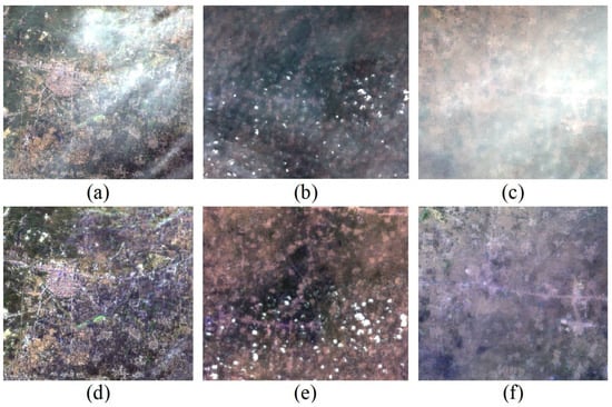
Figure 10.
Dehazing results (sub-scenes) of MODEL-O. (a–c) hazy sub-scenes cut out from a full scene (path 123, row 033, acquisition date 23 September 2015); (d–f) dehazed images using MODEL-O.
Figure 11 shows the dehazing results using MODEL-T. The three hazy images are from different scenes near the training samples in D2. Figure 11a,b covers rich vegetation while the surface in Figure 11c is much barer. The effect of the haze has been eliminated completely, and all surface covers, including bare soil, building areas, vegetation, water body etc., exhibit the proper color. As the training dataset contains samples for the water body, MODEL-T removes haze over the river properly, as shown in Figure 11e,f. MODEL-T handles these situations properly, implying that MRCNN gets the ability to solve new problems through transferring learning.
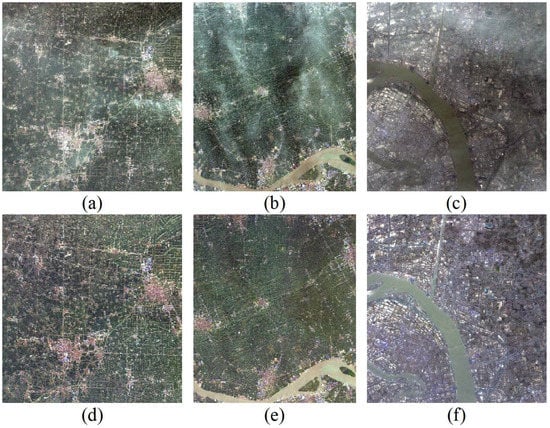
Figure 11.
Dehazing results (sub-scenes) of MODEL-T. (a) hazy block (path 119, row 037, acquisition date 22 April 2016); (b) hazy block (path 119, row 038, acquisition date 22 July 2014); (c) hazy block (path 119, row 038, acquisition date 2 February 2016); (d–f) dehazed images using MODEL-T.
Figure 12 shows the results of four full-size images affected by haze or transparent clouds using MODEL-T. Visually, hazy regions are recovered successfully, and clear regions remain unchanged. Although Figure 12a,b are far away from the training area and show different characteristics, MODEL-T succeeds in removing the haze over them, proving that MODEL-T inherits the learned knowledge of MODEL-O. Since MRCNN extracts abstract features of input images for prediction, MODEL-T does well in removing the haze over apparently different water bodies in Figure 11b,c and Figure 12c,d, even though training samples only contain one kind of water body, similar to Figure 11b.
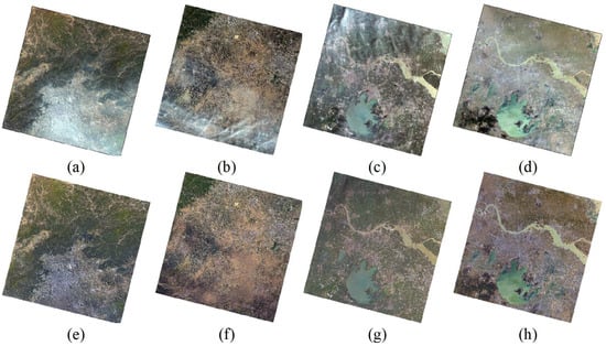
Figure 12.
Dehazing results of full-size Landsat 8 OLI data using MODEL-T. (a–d) original hazy images with spatially varying haze or clouds; (a) path 123, row 032, acquisition date 3 October 2013; (b) path 123, row 033, acquisition date 7 May 2015; (c) path 119, row 038, (d) acquisition date 22 July 2017; path 119, row 038, acquisition date 29 December 2014); (e–h) dehazed images.
Figure 13 shows the dehazing results in the coastal/aerosol band and near-infrared band of Landsat 8 OLI data. Obviously, the effect of haze has been eliminated, and the visibility of the results has been significantly enhanced.
5. Discussion
5.1. Model Performance
The estimation of the haze transmission map is of the greatest importance for haze removal. Its accuracy is directly related to the quality of dehazed images. To validate the accuracy of the proposed MRCNN for the prediction of haze transmission of RS images, the novel network is compared with DehazeNet [30] and VGGNet [57]. DehazeNet was originally designed for natural images and has five weight layers. We use the same network architecture except for replacing the BReLU [61] activation function with the Sigmoid [62] function, based on the experimental fact that the network is difficult to converge when using BReLU. VGGNet is designed for the image classification task. Herein, we adopt a network that has 16 weight layers and remove the softmax classifier to fit the regression problem. The proposed MRCNN has 13 weight layers, which achieves a balance between the network depth and trainable parameters. Three models are initialized in the same way and trained using the same datasets and method.
The qualities of the trained networks can be reflected by learning curves. As shown in Figure 14a, the training errors of the three networks reduce quickly and finally reach a relatively stable state. The speed of convergence for MRCNN is faster than that for DehazeNet and VGGNet. Compared with DehazeNet and VGGNet, the validation error of MRCNN declines more quickly and achieves a more stable state. With further training, the validation error for VGGNet and MRCNN varies between increasing and decreasing but can reduce to a lower value, indicating that the networks are trying to search for better solutions, while it decreases the original level for DehazeNet, implying that the network converges to a local minimum in the end, and the learning process is apparently slowed down. The smaller amplitude of oscillation in the validation error indicates that MRCNN is much easier to adjust. When applying the trained networks for a new dataset, MRCNN can achieve the best result as shown in Figure 14c,d, originally with 0.0294% training error and 0.1455% validation error. Fine-tuning can improve the performance of the networks. Finally, DehazeNet, VGGNet, and MRCNN can obtain the best validation error of 0.0317%, 0.0310%, and 0.0168%, respectively. The validation error of VGGNet remains approximately unchanged after 20 epochs, indicating that the network might have encountered a bottleneck. We further validate the feasibility of the transferring application using a small number of training samples. We divide the dataset D2 into a 30% training set and a 70% testing set. It takes approximately about 13.76 min to fine-tune MRCNN. The best validation score is 0.0179% obtained at epoch 45, with a test performance of 0.0193%. The accuracy is close to that of MODEL-T, but the training time is reduced greatly. The similar experiments are performed for DehazeNet and VGGNet. Their training errors closely approaches 0.035% after 100-epoch of fine-tuning, while the validation and testing errors remain stable at over 0.04% without further improvement.
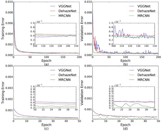
Figure 14.
Learning curves for DehazeNet, VGGNet, and the proposed MRCNN. (a,b) training error and validation error on D1 during the original training process; (c,d) training error and validation error on D2 during the transferring application.
Figure 15 plots the predicted value versus the true transmission on the testing set. The first row corresponds to the results of the trained networks using D1, and the second row shows the results of the fine-tuned networks using D2. The testing errors of different networks are labeled at the upper left of each sub-plot. The predicted values of DehazeNet are lower than the truth values when the real transmissions are close to 1. The center line of VGGNet is discrete, meaning that some transmissions are missed in the prediction result. For MRCNN, the predicted values are centered on the 45-degree line, and the testing errors are lower than that of other networks. In fact, DehazeNet is inherently a shallow network and the extracted features are still low-level. The network generally suffers from different surface types so that the trained network is unable to handle other images in most cases. VGGNet, a deep learning architecture, is capable of extracting high-level, hierarchical, and abstract features to avoid the influence from the surface coverage. However, the high-level features tend to lose weak information and local details, resulting in difficulties for achieving accurate haze transmission estimation. In contrast, MRCNN takes advantage of the multi-scale context aggregation and residual learning to balance between deepening the depth of network and preventing information loss. The trained or fine-tuned MRCNN can achieve higher prediction accuracy than other networks. Although the three networks can obtain a similar final training error, MRCNN converges faster and achieves better validation errors and testing errors during the original training and transferring application.
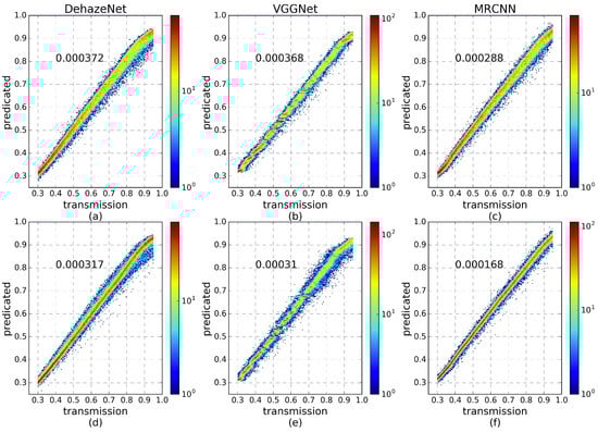
Figure 15.
The density plots between the predicted and truth transmission for DehazeNet, VGGNet, and the proposed MRCNN. (a–c) the results using the testing set of D1 during the original training process; (d–f) the results using the testing set of D2 during transferring learning.
5.2. Analysis of Spectral Consistency
It is difficult to evaluate a single-image based haze removal method quantitatively as the ground information corresponding to the hazy image is usually unknown. Therefore, we choose a pair of hazy and haze-free images that have minimal time difference and a minimal difference of sun/sensor geometry for our evaluation. The spectra of images are compared in two aspects: (1) the difference between the hazy image and the dehazed result in clear regions must be minimal; and (2) the spectra of the dehazed result and the haze-free image are highly similar. Figure 16 illustrates the dehazing result (Figure 16b) of a hazy image (Figure 16a) and the selected haze-free image (Figure 16c). The hazy and haze-free data were acquired with a time difference of 16 days. The dehazed image exhibits good recovery of the surface except slight residual under heavy hazy regions.
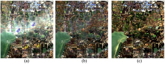
Figure 16.
Comparison of dehazing result and haze-free image: (a) hazy image (path: 119, row: 038, acquisition date: 1 January 2016); (b) dehazed image using MODEL-T; (c) haze-free image (path: 119, row: 038, acquisition date: 16 December 2015).
Figure 17 illustrates the spectra of pixels collected in hazy (asterisk), dehazed (plus), and haze-free (diamond) image. Figure 17a,b are spectral profiles of pixels (cross 1 and 2 in Figure 17a) located in clear regions. The spectra of different images have the same shape and similar DN value, proving that dehazing does not modify the spectral properties in clear regions. Figure 17c,d show spectral profiles of pixels (cross 3 and 4 in Figure 17a) located in hazy regions. The spectra of different images have a similar shape. The DN values of the dehazed and haze-free image are in close agreement but are different from the hazy image. This suggests that dehazing adjusts the radiances of hazy pixels to a certain degree and produces a spectrally consistent result.
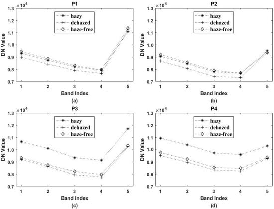
Figure 17.
Spectral profiles of pixels in hazy (asterisk), dehazed (plus) and haze-free (diamond) images. The location of sampled pixels is marked by cross 1–4 in Figure 8a. (a–d) spectra corresponding to cross 1 to 4, respectively. The X-axis is band index and Y-axis is DN (digital numbers) value.
Figure 18 presents the blue and red band profiles of hazy (red line), dehazed (green line), and haze-free (blue line) images. Along the vertical line, the hazy image is relatively clear on both sides while affected by haze in the middle. Correspondingly, the left and right parts of Figure 18a,c have similar shapes and DN values, while the middle parts are different. Along the horizontal line, the image is entirely covered by haze. In Figure 18b,d, the curves of the hazy image are remarkably different from the others. In contrast, the spectra of the dehazed and haze-free image are highly overlapping. This indicates that dehazing maintains the similarity in clear regions properly and reveals a noticeable enhancement in hazy regions. The remaining differences can be attributed to residual haze, different atmospheric conditions, or a change of surface.
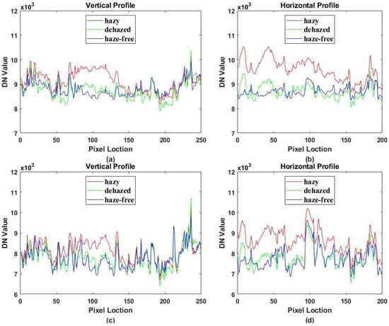
Figure 18.
Band profiles taken from hazy (red line), dehazed (green line) and haze-free (blue line) images. The location is marked by the red cross in Figure 8a. (a) vertical profile of blue band (0.483 μm); (b) horizontal profile of blue band; (c) vertical profile of red band (0.655 μm); (d) horizontal profile of red band.
5.3. Influence on Vegetation Index
Spectral consistency of dehazing results ensures that haze removal would not affect the algorithms that rely on the spectral information of remote sensing images. The dehazed images are expected to be used as data sources of land cover classification and mapping, surface change detection and other applications involving ground information extraction. Herein, we implement a test of extracting vegetation using the normalized difference vegetation index (NDVI) from the original hazy image, dehazed image, and haze-free reference image respectively. The expression of NDVI is written as:
where is the reflectivity for the indicated band, and stands for band NIR and red, respectively.
An example is given in Figure 19. The original hazy image, covering the urban and suburban areas of Beijing, was acquired on 19 August 2014 and processed with MODEL-T. The haze-free reference image is on 4 September 2014, having a minimal time difference with the hazy image. Both the original hazy or clear image and the dehazing result are run for atmospheric correction in FLAASH [63] module in ENVI software. Figure 19a–c shows the corrected results for the hazy image, dehazing result, and reference image respectively. Figure 19d–f are classification results using an NDVI threshold of 0.5. In this period, the vegetation in the north finishes growing and begins withering, while a comparison of Figure 19d,f displays a rapid growth of vegetation, which defies the common sense. Due to the influence of haze, NDVI of the hazy image is smaller than that of the usual, leading to neglection of some vegetation with a usual threshold. In contrast, the comparison of Figure 19e,f is much closer to the truth, which reflects a reduction of vegetation with the arrival of autumn. In fact, when adjusting the threshold of Figure 19d to 0.35, we reach the same conclusion as Figure 19e, with 66.74% of vegetation. It indicates that NDVI is strongly influenced by severe haze conditions, and haze removal can corrected the bias to some degree.
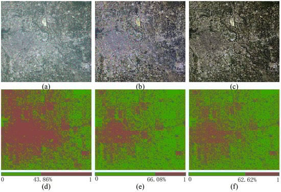
Figure 19.
Atmospheric correction of dehazing results: (a) hazy image (path: 123, row: 032, acquisition date: 19 August 2014); (b) dehazed image using MODEL-T; (c) haze-free image (path: 123, row: 032, acquisition date: 4 September 2014); (d–f) classification results of a-c respectively; the green represents pixels whose NDVI are equal to or larger than 0.5; the brown represents pixels whose NDVI are smaller than 0.5; the numbers at the bottom indicate the percentage of vegetation.
6. Conclusions
We present a multi-scale residual convolutional neural network (MRCNN), which takes advantage of both spatial and spectral information for haze removal of remote sensing images. The overall architecture mainly contains four sequential modules: (1) spectral–spatial feature extraction, which utilizes 3D convolutional kernels to extract spatial–spectral correlation information; (2) multi-scale context aggregation, which uses dilated convolution is used to capture abstract features in different receptive fields and aggregate multi-scale contextual information without losing resolution; (3) residual learning, which avoids the loss of weak information while deepening the network for high-level features; and (4) fully connected layers, which take advantage of dropout to improve the generalization ability and prevent overfitting. The network takes hazy patches as input and outputs haze transmission. The training datasets are generated from clear image blocks by simulating the haze degradation process. Considering the difficulty of building a complete dataset containing various kinds of surface cover types, clear samples are collected in a local clear region of a single scene in our experiments. MRCNN is trained through mini-batch stochastic gradient descent (MSGD) and an early-stopping mechanism to minimize the mean squared error between the predicted values and truth haze transmissions. After finishing training, the network is capable of predicting the haze transmission of hazy images in surrounding areas. Post-processing is necessary for the correction of the latent residual of dehazed images. The trained network can be reinforced and fine-tuned by means of further learning from new samples collected in other areas during the transferring application. The optimization costs little time since the initialized parameters have learned sufficient knowledge in the previous stage. The fine-tuned network not only gains the ability to solve new problems but also inherits the ability of the previous network. The trained network can extend its applicability constantly through transferring learning.
Experiments show that the trained network can achieve a validation score of 0.0289% and testing performance of 0.0288% during the original training, and 0.1455% validation error during transferring application, which can reach 0.0168% with further fine-tuning. Taking advantage of the multi-scale context aggregation and residual learning, MRCNN converges faster and can achieve a higher prediction accuracy compared with DehazeNet [30] and VGGNet [57]. We selected several scenes of Landsat 8 OLI data for haze removal. The result of image quality assessment indicates that the trained MRCNN is state-of-the-art to obtain dehazed images, whose color is consistent with the actual scene. Compared with the traditional methods based on different priors, the proposed MRCNN owns more powerful generalization ability. Since MRCNN extracts high-level, hierarchical, and abstract features for haze transmission estimation, it hardly suffers from different surface types and various haze or thin clouds. Meanwhile, MRCNN is able to preserve structural information, and prevent the loss of correlation, luminance distortion and contrast distortion of images.
A comparison to haze-free reference data reveals that the dehazing process maintains the proper similarity in clear regions and produces a noticeable enhancement in hazy regions. In addition, the spectral consistency of dehazing results ensures that haze removal would not affect algorithms that rely on the spectral information of remote sensing images.
Author Contributions
N.L. conceived and designed the experiments; H.J. performed the experiments and wrote the paper.
Funding
This work was supported by the Young Talent Fund of Institute of Geographic Sciences and Natural Resources Research (2015RC203).
Acknowledgments
The Landsat 8 OLI data were obtained from the Global Visualization Viewer of the United States Geological Survey (USGS).
Conflicts of Interest
The authors declare no conflict of interest. The founding sponsors had no role in the design of the study; in the collection, analyses, or interpretation of data; in the writing of the manuscript, or in the decision to publish the results.
References
- Chavez, P.S. An improved dark-object subtraction technique for atmospheric scattering correction of multispectral data. Remote Sens. Environ. 1988, 24, 459–479. [Google Scholar] [CrossRef]
- Chavez, P.S. Image-based atmospheric corrections revisited and improved. Photogramm. Eng. Remote Sens. 1996, 62, 1025–1036. [Google Scholar]
- Liang, S.; Fang, H.; Chen, M. Atmospheric correction of Landsat ETM+ land surface imagery. I. Methods. IEEE Trans. Geosci. Remote Sens. 2001, 39, 2490–2498. [Google Scholar] [CrossRef]
- Liang, S.; Fang, H.; Morisette, J.T.; Chen, M.; Shuey, C.J.; Walthall, C.; Daughtry, C.S.T. Atmospheric correction of Landsat ETM+ land surface imagery: II. Validation and applications. IEEE Trans. Geosci. Remote Sens. 2002, 40, 2736–2746. [Google Scholar] [CrossRef]
- Zhang, Y.; Guindon, B.; Cihlar, J. An image transform to characterize and compensate for spatial variations in thin cloud contamination of Landsat images. Remote Sens. Environ. 2002, 82, 173–187. [Google Scholar] [CrossRef]
- He, X.Y.; Hu, J.B.; Chen, W.; Li, X.Y. Haze removal based on advanced haze-optimized transformation (AHOT) for multispectral imagery. Int. J. Remote Sens. 2010, 31, 5331–5348. [Google Scholar] [CrossRef]
- Jiang, H.; Lu, N.; Yao, L. A high-fidelity haze removal method based on hot for visible remote sensing images. Remote Sens. (Basel) 2016, 8, 844. [Google Scholar] [CrossRef]
- Chen, S.L.; Chen, X.H.; Chen, J.; Jia, P.F.; Cao, X.; Liu, C.Y. An iterative haze optimized transformation for automatic cloud/haze detection of Landsat imagery. IEEE Trans. Geosci. Remote Sens. 2016, 54, 2682–2694. [Google Scholar] [CrossRef]
- Sun, L.X.; Latifovic, R.; Pouliot, D. Haze removal based on a fully automated and improved haze optimized transformation for Landsat imagery over land. Remote Sens. (Basel) 2017, 9, 972. [Google Scholar]
- Liu, C.; Hu, J.; Lin, Y.; Wu, S.; Huang, W. Haze detection, perfection and removal for high spatial resolution satellite imagery. Int. J. Remote Sens. 2011, 32, 8685–8697. [Google Scholar] [CrossRef]
- Makarau, A.; Richter, R.; Muller, R.; Reinartz, P. Haze detection and removal in remotely sensed multispectral imagery. IEEE Trans. Geosci. Remote Sens. 2014, 52, 5895–5905. [Google Scholar] [CrossRef]
- Makarau, A.; Richter, R.; Schlapfer, D.; Reinartz, P. Combined haze and cirrus removal for multispectral imagery. IEEE Geosci. Remote Sens. Lett. 2016, 13, 379–383. [Google Scholar] [CrossRef]
- Shen, H.F.; Li, H.F.; Qian, Y.; Zhang, L.P.; Yuan, Q.Q. An effective thin cloud removal procedure for visible remote sensing images. ISPRS J. Photogramm. 2014, 96, 224–235. [Google Scholar] [CrossRef]
- Mitchell, O.R.; Delp, E.J.; Chen, P.L. Filtering to remove cloud cover in satellite imagery. IEEE Trans. Geosci. Electron. 1977, 15, 137–141. [Google Scholar] [CrossRef]
- He, K.; Sun, J.; Tang, X. Single image haze removal using dark channel prior. IEEE Trans. Pattern Anal. Mach. Intell. 2011, 33, 2341–2353. [Google Scholar] [PubMed]
- Xie, B.; Guo, F.; Cai, Z. Improved single image dehazing using dark channel prior and multi-scale retinex. In Proceedings of the 2010 International Conference on Intelligent System Design and Engineering Application, Changsha, China, 13–14 October 2010; pp. 848–851. [Google Scholar]
- Zhu, Q.; Yang, S.; Heng, P.A.; Li, X. An adaptive and effective single image dehazing algorithm based on dark channel prior. In Proceedings of the 2013 IEEE International Conference on Robotics and Biomimetics, Shenzhen, China, 12–14 December 2013; pp. 1796–1800. [Google Scholar]
- Xiao, C.; Gan, J. Fast image dehazing using guided joint bilateral filter. Vis. Comput. 2012, 28, 713–721. [Google Scholar] [CrossRef]
- He, K.; Sun, J.; Tang, X. Guided image filtering. In Proceedings of the 2010 European Conference on Computer Vision, Heraklion, Greece, 5–11 September 2010; pp. 1–14. [Google Scholar]
- Tarel, J.P.; Hautière, N. Fast visibility restoration from a single color or gray level image. In Proceedings of the 2009 IEEE International Conference on Computer Vision, Kyoto, Japan, 29 September–2 October 2009; pp. 2201–2208. [Google Scholar]
- Long, J.; Shi, Z.W.; Tang, W.; Zhang, C.S. Single remote sensing image dehazing. IEEE Geosci Remote Sens. 2014, 11, 59–63. [Google Scholar] [CrossRef]
- Pan, X.; Xie, F.; Jiang, Z.; Yin, J. Haze removal for a single remote sensing image based on deformed haze imaging model. IEEE Signal Process. Lett. 2015, 22, 1806–1810. [Google Scholar] [CrossRef]
- Jiang, H.; Lu, N.; Yao, L.; Zhang, X.X. Single image dehazing for visible remote sensing based on tagged haze thickness maps. Remote Sens. Lett. 2018, 9, 627–635. [Google Scholar] [CrossRef]
- Tang, K.T.; Yang, J.C.; Wang, J. Investigating haze-relevant features in a learning framework for image dehazing. In Proceedings of the 2014 IEEE Conference on Computer Vision and Pattern Recognition (CVPR), Beijing, China, 23–28 June 2014; pp. 2995–3002. [Google Scholar]
- Breiman, L. Random forests. Mach. Learn. 2001, 45, 5–32. [Google Scholar] [CrossRef]
- Zhu, Q.S.; Mai, J.M.; Shao, L. A fast single image haze removal algorithm using color attenuation prior. IEEE Trans. Image Process. 2015, 24, 3522–3533. [Google Scholar] [PubMed]
- Schuler, C.J.; Burger, H.C.; Harmeling, S.; Scholkopf, B. A machine learning approach for non-blind image deconvolution. In Proceedings of the 2013 IEEE Conference on Computer Vision and Pattern Recognition (CVPR), Portland, OR, USA, 23–28 June 2013; pp. 1067–1074. [Google Scholar]
- Eigen, D.; Krishnan, D.; Fergus, R. Restoring an image taken through a window covered with dirt or rain. In Proceedings of the 2013 IEEE International Conference on Computer Vision (ICCV), Sydney, Australia, 1–8 December 2013; pp. 633–640. [Google Scholar]
- Dong, C.; Chen, C.L.; He, K.; Tang, X. Image super-resolution using deep convolutional networks. IEEE Trans. Pattern Anal. Mach. Intell. 2016, 38, 295–307. [Google Scholar] [CrossRef] [PubMed]
- Cai, B.L.; Xu, X.M.; Jia, K.; Qing, C.M.; Tao, D.C. Dehazenet: An end-to-end system for single image haze removal. IEEE Trans. Image Process. 2016, 25, 5187–5198. [Google Scholar] [CrossRef] [PubMed]
- Ghamisi, P.; Chen, Y.S.; Zhu, X.X. A self-improving convolution neural network for the classification of hyperspectral data. IEEE Geosci. Remote Sens. 2016, 13, 1537–1541. [Google Scholar] [CrossRef]
- Yang, J.X.; Zhao, Y.Q.; Chan, J.C.W.; Yi, C. Hyperspectral image classification using two-channel deep convolutional neural network. In Proceedings of the 2016 IEEE International Geoscience and Remote Sensing Symposium (IGARSS), Beijing, China, 10–15 July 2016; pp. 5079–5082. [Google Scholar]
- Paoletti, M.E.; Haut, J.M.; Plaza, J.; Plaza, A. A new deep convolutional neural network for fast hyperspectral image classification. ISPRS J. Photogramm. Remote Sens. 2017. [Google Scholar] [CrossRef]
- Sherrah, J. Fully convolutional networks for dense semantic labelling of high-resolution aerial imagery. arXiv, 2016; arXiv:1606.02585. [Google Scholar]
- Liu, Y.; Fan, B.; Wang, L.; Bai, J.; Xiang, S.; Pan, C. Semantic labeling in very high resolution images via a self-cascaded convolutional neural network. ISPRS J. Photogramm. Remote Sens. 2017. [Google Scholar] [CrossRef]
- Langkvist, M.; Kiselev, A.; Alirezaie, M.; Loutfi, A. Classification and segmentation of satellite orthoimagery using convolutional neural networks. Remote Sens. (Basel) 2016, 8, 329. [Google Scholar] [CrossRef]
- Zhou, B.; Khosla, A.; Lapedriza, A.; Oliva, A.; Torralba, A. Object detectors emerge in deep scene cnns. Comput. Sci. 2014, arXiv:1412.6856. [Google Scholar]
- Diao, W.; Sun, X.; Dou, F.; Yan, M.; Wang, H.; Fu, K. Object recognition in remote sensing images using sparse deep belief networks. Remote Sens. Lett. 2015, 6, 745–754. [Google Scholar] [CrossRef]
- Pacifici, F.; Frate, F.D.; Solimini, C.; Emery, W.J. An innovative neural-net method to detect temporal changes in high-resolution optical satellite imagery. IEEE Trans. Geosci. Remote Sens. 2007, 45, 2940–2952. [Google Scholar] [CrossRef]
- Narasimhan, S.G.; Nayar, S.K. Vision and the atmosphere. Int. J. Comput. Vis. 2002, 48, 233–254. [Google Scholar] [CrossRef]
- Narasimhan, S.G.; Nayar, S.K. Contrast restoration of weather degraded images. IEEE Trans. Pattern Anal. 2003, 25, 713–724. [Google Scholar] [CrossRef]
- Cun, Y.L.; Boser, B.; Denker, J.S.; Howard, R.E.; Habbard, W.; Jackel, L.D.; Henderson, D. Handwritten digit recognition with a back-propagation network. Adv. Neural Inf. Process. Syst. 1990, 2, 396–404. [Google Scholar]
- Nair, V.; Hinton, G.E. Rectified linear units improve restricted boltzmann machines. In Proceedings of the 2010 International Conference on International Conference on Machine Learning, Haifa, Israel, 21–24 June 2010; pp. 807–814. [Google Scholar]
- Glorot, X.; Bordes, A.; Bengio, Y. Deep sparse rectifier neural networks. JMLR W & CP 2012, 15, 315–323. [Google Scholar]
- Glorot, X.; Bengio, Y. Understanding the difficulty of training deep feedforward neural networks. J. Mach. Learn. Res. 2010, 9, 249–256. [Google Scholar]
- Krizhevsky, A.; Sutskever, I.; Hinton, G.E. Imagenet classification with deep convolutional neural networks. In Proceedings of the International Conference on Neural Information Processing Systems, Lake Tahoe, NV, USA, 3–8 December 2012; pp. 1097–1105. [Google Scholar]
- Ancuti, C.O.; Ancuti, C.; Hermans, C.; Bekaert, P. A fast semi-inverse approach to detect and remove the haze from a single image. Lect. Notes Comput. Sci. 2011, 6493, 501–514. [Google Scholar]
- Li, Y.; Zhang, H.K.; Shen, Q. Spectral-spatial classification of hyperspectral imagery with 3D convolutional neural network. Remote Sens. (Basel) 2017, 9, 67. [Google Scholar] [CrossRef]
- Goodfellow, I.J.; Warde-Farley, D.; Mirza, M.; Courville, A.; Bengio, Y. Maxout networks. In Proceedings of the 2013 ICML, Atlanta, GA, USA, 16–21 June 2013; pp. 1319–1327. [Google Scholar]
- Yu, F.; Koltun, V. Multi-scale context aggregation by dilated convolutions. arXiv, 2015; arXiv:1511.07122. [Google Scholar]
- He, K.M.; Zhang, X.Y.; Ren, S.Q.; Sun, J. Spatial pyramid pooling in deep convolutional networks for visual recognition. In Computer Vision—ECCV 2014, Pt III; Springer: Cham, Switzerland, 2014; Volume 8691, pp. 346–361. [Google Scholar]
- He, K.M.; Zhang, X.Y.; Ren, S.Q.; Sun, J. Deep residual learning for image recognition. In Proceedings of the 2016 IEEE Conference on Computer Vision and Pattern Recognition (CVPR), Las Vegas, NV, USA, 27–30 June 2016; pp. 770–778. [Google Scholar]
- Hinton, G.E.; Srivastava, N.; Krizhevsky, A.; Sutskever, I.; Salakhutdinov, R.R. Improving neural networks by preventing co-adaptation of feature detectors. Comput. Sci. 2012, 3, 212–223. [Google Scholar]
- Srivastava, N.; Hinton, G.; Krizhevsky, A.; Sutskever, I.; Salakhutdinov, R. Dropout: A simple way to prevent neural networks from overfitting. J. Mach. Learn. Res. 2014, 15, 1929–1958. [Google Scholar]
- Chollet, F. Keras. Available online: http://keras-cn.readthedocs.io/en/latest (accessed on 12 January 2018).
- Team, T.D.; Alrfou, R.; Alain, G.; Almahairi, A.; Angermueller, C.; Bahdanau, D.; Ballas, N.; Bastien, F.; Bayer, J.; Belikov, A. Theano: A python framework for fast computation of mathematical expressions. arXiv, 2017; arXiv:1605.02688. [Google Scholar]
- Simonyan, K.; Zisserman, A. Very deep convolutional networks for large-scale image recognition. Comput. Sci. 2014, arXiv:1409.1556. [Google Scholar]
- Sheikh, H.R.; Bovik, A.C. Image information and visual quality. IEEE Trans. Image Process. 2006, 15, 430–444. [Google Scholar] [CrossRef] [PubMed]
- Wang, Z.; Bovik, A.C. A universal image quality index. IEEE Signal Process. Lett. 2002, 9, 81–84. [Google Scholar] [CrossRef]
- Wang, Z.; Bovik, A.C.; Sheikh, H.R.; Simoncelli, E.P. Image quality assessment: From error visibility to structural similarity. IEEE Trans. Image Process. 2004, 13, 600–612. [Google Scholar] [CrossRef] [PubMed]
- Wu, Z.; Lin, D.; Tang, X. Adjustable bounded rectifiers: Towards deep binary representations. Comput. Sci. 2015, arXiv:1511.06201. [Google Scholar]
- Hinton, G.E.; Salakhutdinov, R.R. Reducing the dimensionality of data with neural networks. Science 2006, 313, 504–507. [Google Scholar] [CrossRef] [PubMed]
- Cooley, T.; Anderson, G.P.; Felde, G.W.; Hoke, M.L.; Ratkowski, A.J.; Chetwynd, J.H.; Gardner, J.A.; Adler-Golden, S.M.; Matthew, M.W.; Berk, A.; et al. Flaash, a modtran4-based atmospheric correction algorithm, its application and validation. Int. Geosci. Remote Sens. 2002, 3, 1414–1418. [Google Scholar]
© 2018 by the authors. Licensee MDPI, Basel, Switzerland. This article is an open access article distributed under the terms and conditions of the Creative Commons Attribution (CC BY) license (http://creativecommons.org/licenses/by/4.0/).