IMF-Slices for GPR Data Processing Using Variational Mode Decomposition Method

Abstract

Using traditional time-frequency analysis methods, it is possible to delineate the time-frequency structures of ground-penetrating radar (GPR) data. A series of applications based on time-frequency analysis were proposed for the GPR data processing and imaging. With respect to signal processing, GPR data are typically non-stationary, which limits the applications of these methods moving forward. Empirical mode decomposition (EMD) provides alternative solutions with a fresh perspective. With EMD, GPR data are decomposed into a set of sub-components, i.e., the intrinsic mode functions (IMFs). However, the mode-mixing effect may also bring some negatives. To utilize the IMFs’ benefits, and avoid the negatives of the EMD, we introduce a new decomposition scheme termed variational mode decomposition (VMD) for GPR data processing for imaging. Based on the decomposition results of the VMD, we propose a new method which we refer as “the IMF-slice”. In the proposed method, the IMFs are generated by the VMD trace by trace, and then each IMF is sorted and recorded into different profiles (i.e., the IMF-slices) according to its center frequency. Using IMF-slices, the GPR data can be divided into several IMF-slices, each of which delineates a main vibration mode, and some subsurface layers and geophysical events can be identified more clearly. The effectiveness of the proposed method is tested using synthetic benchmark signals, laboratory data and the field dataset.

1. Introduction

Most of the geophysical data are non-stationary. Especially for the ground-penetrating radar (GPR) data, which can be treated as a set of time-series signals, such non-stationarity appears more obviously. Non-stationarity can be defined and measured by certain statistical methods [1], however, geophysicists are prone to using the time-frequency decomposition methods (e.g., wavelet transform [2,3], S-transform [4,5] and matching pursuit [6,7]) to delineate the non-stationary characteristics. This is because these methods provide a visualization and are convenient for further applications.

Recently, empirical mode decomposition (EMD) has been providing alternative solutions with a fresh perspective. With EMD-based methods, the GPR data can be decomposed into a group of stationary sub-components (i.e., intrinsic mode functions, IMFs), and the subsequent processing for subsurface information is thus focused on the analysis of the generated IMFs instead [8]. The decomposed IMFs of GPR data highlight two important features. The first is that the IMFs are close to being stationary. This leads to a direct application of time-frequency analysis of GPR data [9], in which time-frequency structures can be computed steadily within each IMF. The other feature is that the decomposed IMFs correspond to different frequency bands or ranges. This means that any operation performed on the IMFs (e.g., removing or extracting a few IMFs) amounts to filtering in the corresponding frequency domain. In this regard, the derived applications based on IMFs may include denoising [10], subsurface objects identification [11], etc. However, the mode-mixing effect and the lack of a mathematical foundation limit their further applications in GPR data processing and imaging.

To utilize the benefits of the IMFs mentioned above, and avoid the negatives of the EMD, we introduce a new decomposition scheme called variational mode decomposition (VMD) [12] for GPR data processing as well as for imaging. The VMD decomposition is not “empirical” any more, while the mathematical framework is well-established. Specifically, though the decomposition results can still be seen as IMFs, the computation is implemented by solving an optimization problem. Some references have demonstrated that the VMD is able to avoid mode-mixing phenomena [13,14,15], and therefore the decomposition results match the input signal’s intrinsic vibration mode better. In this study, we test VMD decomposition on GPR data, and based on the VMD decomposition results, we propose a new method for GPR imaging which we refer as “the IMF-slice”. In the proposed method, the IMFs are generated by the VMD trace by trace, and then each IMF is sorted and recorded into different profiles (i.e., the IMF-slice) according to its center frequency. A GPR profile could be divided into several IMF-slices, each of which delineates a main vibration mode within certain frequency band. Using IMF-slices, some subsurface events are able to be identified more clearly.

As parts of the long-term study of the mathematical transformations of GPR data, this work shows elementary research on the applications of the VMD decomposition for GPR imaging. The objectives of this work are to: (1) introduce the VMD decomposition and test its feasibility on GPR data; (2) compare the decomposition results of GPR data between the VMD and the classic EMD; (3) propose the concept of IMF-slices and discuss their applications in GPR imaging and interpretation. The paper starts with a methods section introducing the VMD decomposition and the IMF-slices for GPR data. We then show some results based on synthetic benchmark tests, laboratory data tests and a field dataset. Finally, the conclusions and discussions are provided in the last section.

2. Methods

2.1. The Variational Mode Decomposition

The VMD algorithm was initially described as solving the following constrained optimization subject to equality constraints by Dragomiretskiy and Zosso [12],

$$\begin{array}{l}\underset{\left\{u_k\right\},\left\{w_k\right\}}{{\displaystyle \min }}\left\{{\displaystyle \sum _k^{}{\Vert {\partial }_t\left[\left(\delta \left(t\right)+\frac{j}{\pi t}\right)\ast u_k\left(t\right)\right]e^{-j{\omega }_{k}t}\Vert }_2^2}\right\}\\ s.t.{\displaystyle \sum _k^{}{u}_k\left(t\right)}=f\left(t\right)\end{array}$$

(1)

In the above form, $\delta \left(t\right)$ is the Dirac function, and ${\left\{u_k\left(t\right)\right\}}_{k=1,2,\dots N}$ denotes the decomposed sub-components (i.e., the IMFs) embedded in the input signal $f\left(t\right)$, where $k$ identifies the number of IMFs. ${\left\{{\omega }_k\right\}}_{k=1,2,\dots N}$ denotes the corresponding center frequencies of each IMF. Within the Lagangian-multiplier framework, the penalty-term and the Lagangian-multiplier $\lambda$ are introduced. Then the above optimization problem would be turned to solving the defined Lagrange function [16] as follows,

$$\begin{array}{l}L(\{u_k\},\{{\omega }_k\},\lambda )\\ =\alpha {\displaystyle \sum _k^{}{\Vert {\partial }_t\left[\left(\delta \left(t\right)+\frac{j}{\pi t}\right)\ast u_k\left(t\right)\right]e^{-j{\omega }_{k}t}\Vert }_2^2}+{\Vert f\left(t\right)-{\displaystyle \sum _k^{}{u}_k\left(t\right)}\Vert }_2^2+⟨\lambda \left(t\right),f\left(t\right)-{\displaystyle \sum _k^{}{u}_k\left(t\right)}⟩\end{array}$$

(2)

where $L(\{u_k\},\{{\omega }_k\},\lambda )$ denotes the Lagrange function, and the parameter $\alpha$ is used for balancing the reconstruction error. Its solution can be derived by the well-known alternating direction method of multipliers (ADMM) [17].

Assuming that there are K IMFs decomposed, the frequency-domain expression of the kth IMF derived by the VMD is,

$${\widehat{u}}_k^{n+1}(\omega )=\frac{\widehat{f}\left(\omega \right)-{\displaystyle \sum _{i=1}^{k-1}{\widehat{u}}_i^{n+1}\left(\omega \right)}-{\displaystyle \sum _{i=k+1}^K{\widehat{u}}_i^n\left(\omega \right)}+\frac{{\widehat{\lambda }}^n(\omega )}{2}}{1+2\alpha {(\omega -{\omega }_k^n)}^2}$$

(3)

in which $\widehat{f}\left(\omega \right)$, ${\widehat{u}}_i^{}\left(\omega \right)$, $\widehat{\lambda }(\omega )$, and ${\widehat{u}}_k^{n+1}\left(\omega \right)$ are the frequency-domain forms of $f\left(t\right)$, $u_i^{}\left(t\right)$, $\lambda (t)$, $u_k^{n+1}\left(t\right)$ using the Fourier transform, and n denotes iteration number. The criterion of iteration termination is

$${\displaystyle \sum _k{\Vert u_k^{n+1}\left(t\right)-u_k^n\left(t\right)\Vert }_2^2/{\Vert u_k^n\left(t\right)\Vert }_2^2}\le \epsilon ,$$

(4)

where $\epsilon$ denotes the tolerance of convergence. Based on the decomposed IMFs, the input signal can be represented by the decomposed IMFs and the residual signal $r\left(t\right)$,

$$f(t)={\displaystyle \sum _{i=1}^K{u}_i^{n+1}\left(t\right)}+r\left(t\right).$$

(5)

It should be noted that, though the final expansion form of the VMD decomposition (i.e., Equation (5)) is similar to that of the EMD, the computation of each IMF in VMD is totally different. Since the detailed deduction and comparisons with the EMD algorithm are not the main purposes of this paper, we will show the decomposition results in the Section 3.

2.2. IMF-Slices of GPR Data

Compared with traditional common-frequency slices, the IMF-slices can be treated as a set of IMFs. In the VMD scheme, the center frequency ${\omega }_k\left(t\right)$ of each decomposed IMF can be obtained simultaneously. Given a GPR profile (i.e., a B-scan), the IMFs can be derived by VMD trace by trace, where the “trace” here means the A-scan. If we pre-define the frequency intervals or ranges for the IMF-slices, the IMFs of each trace can be classified into different IMF-slices. It should be noted that the frequency ranges for each IMF-slice can be estimated empirically using the center frequencies obtained for each IMF of the first five or ten traces. For example, if the frequency range of a IMF-slice is defined as $\left[{\omega }_1,{\omega }_2\right]$, and combining the median filtering, each decomposed IMF of one trace are evaluated whether it belongs to this range. If yes, it is recorded in the corresponding trace of the IMF-slice, which can be represented as,

$$\mathit{IMF-slice}(x,t)={\displaystyle \sum _{i=1}^K\theta \left(\mathrm{M}\left({\omega }_i\left(t\right)\right)\right)u_i^{}\left(t\right)}$$

(6)

where $\mathrm{M}$ denotes the median filtering operator, and the $\theta$ is the Heaviside function,

$$\theta \left(\omega \right)=\{\begin{array}{l}1,\mathrm{for}\omega \in \left[{\omega }_1,{\omega }_2\right],\\ 0,\mathrm{else}.\end{array}$$

(7)

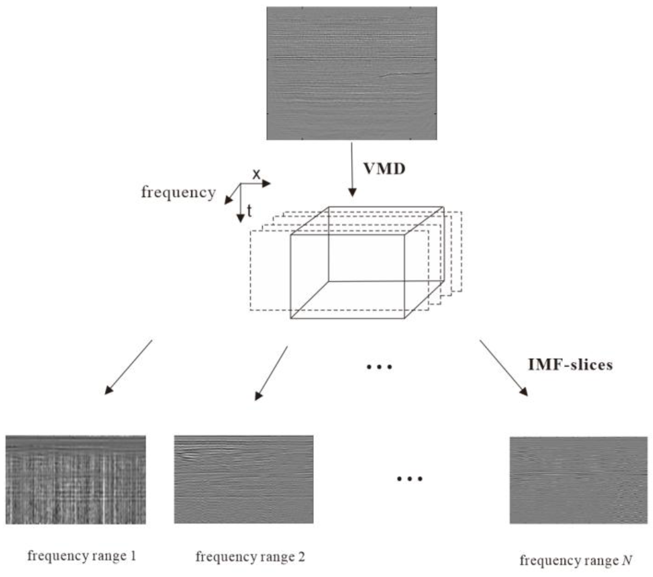
Equation (6) appears to be a band-pass filter for the IMFs. A schematic diagram based on the VMD decomposition is shown in Figure 1.

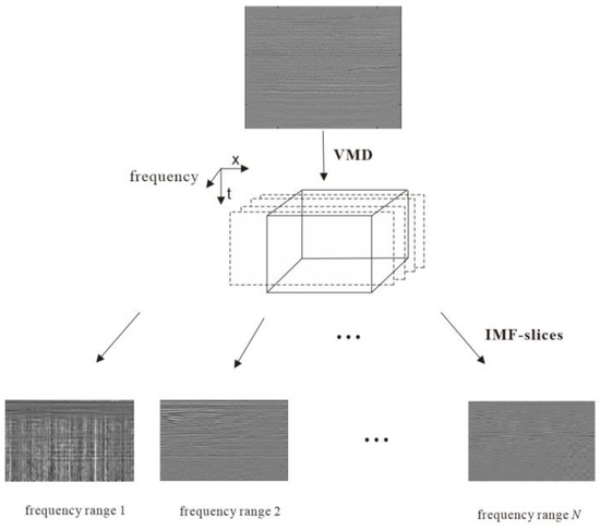
Figure 1. Schematic diagram of IMF-slices.

Similarly, the IMF-slices can be also generated based on EMD. However, since the center frequencies for each IMF, accompanied by the VMD decomposition results, cannot be obtained in the EMD scheme, we select the Taner’s instantaneous frequency [18] to replace it,

$$\omega \left(t\right)=\frac{1}{2\pi }\frac{f_{IMF}\left(t\right)\frac{d{f}_{IMF}{}^{*}\left(t\right)}{dt}-f_{IMF}{}^{*}\left(t\right)\frac{d{f}_{IMF}\left(t\right)}{dt}}{f_{IMF}{}^2\left(t\right)+f_{IMF}{}^{*2}\left(t\right)},$$

(8)

where $f_{IMF}\left(t\right)$ and $f_{IMF}{}^{*}\left(t\right)$ here denotes the IMF and its conjugate form.

3. Results

3.1. Synthetic Benchmark Tests

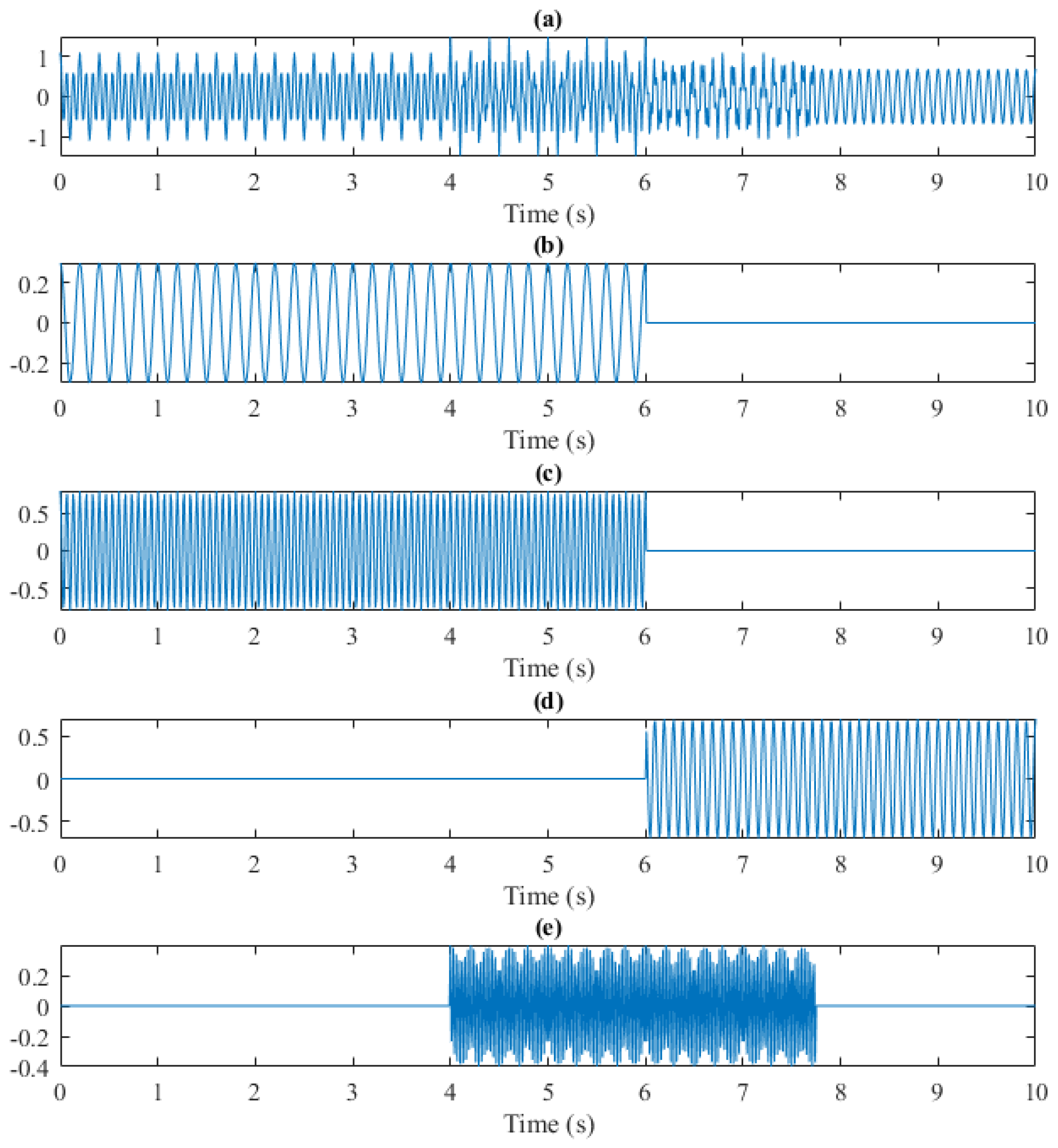
In this section, we firstly test a synthetic benchmark signal formulated by Herrera et al. [19,20], which can be characterized as a non-stationary and multi-component signal. The signal (Figure 2a) is comprised of four sub-components, which are relatively stationary in certain time ranges, see Figure 2b–e. Figure 3 shows the corresponding instantaneous frequencies (IFs).

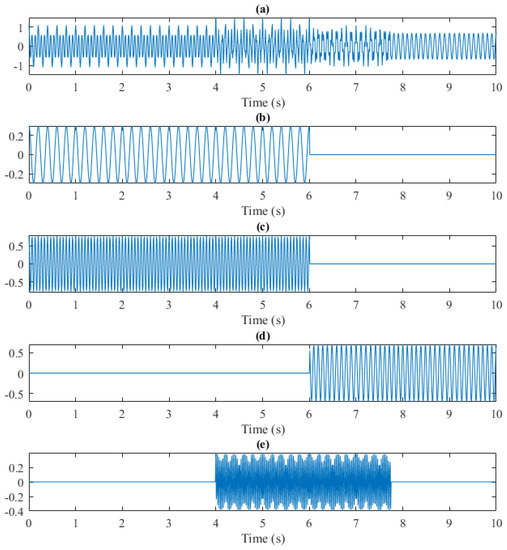
Figure 2. The synthetic data (a) composed of four sub-components (b–e).

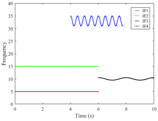
Figure 3. The corresponding instantaneous frequencies of the sub-components in Figure 1.

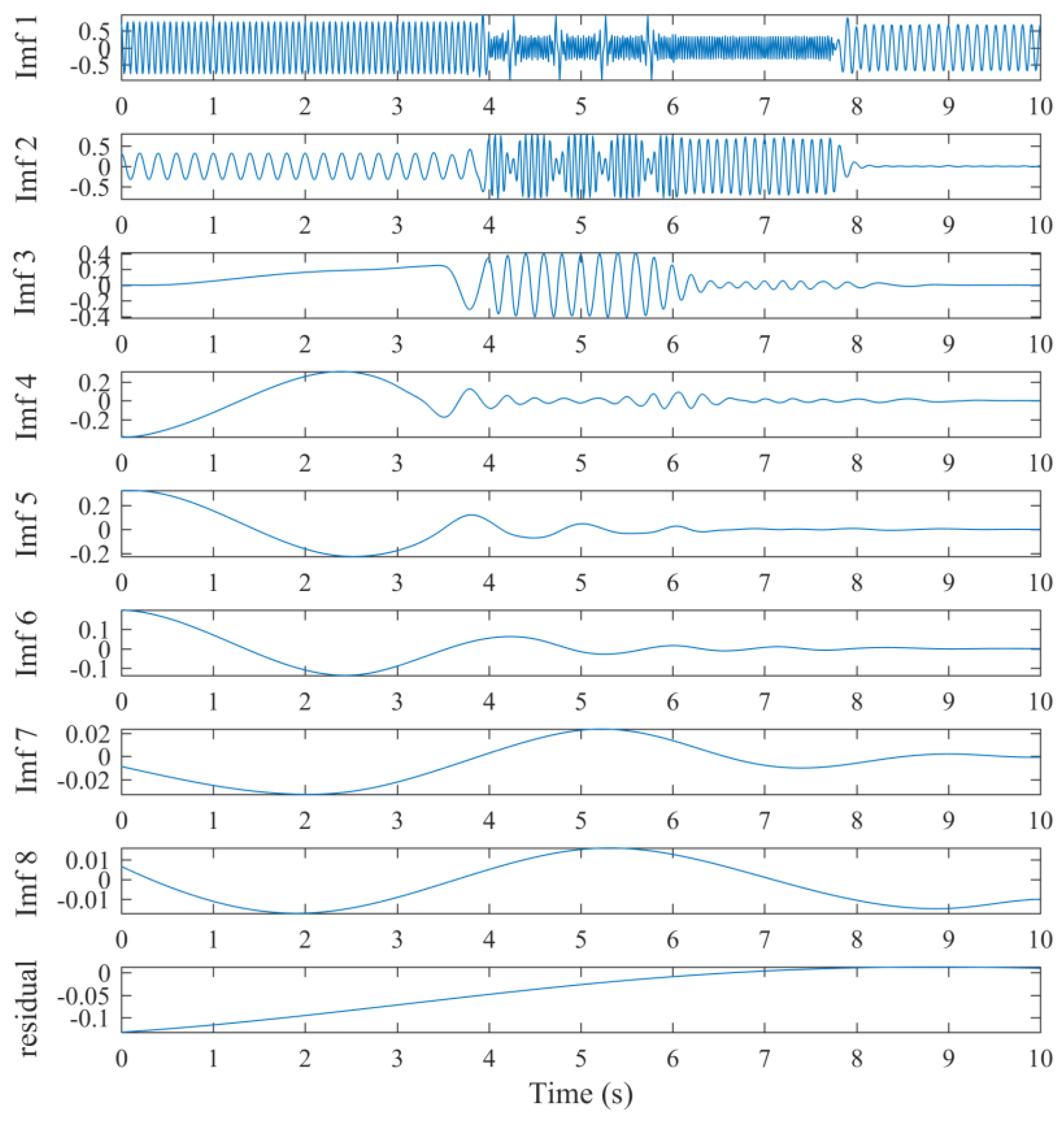
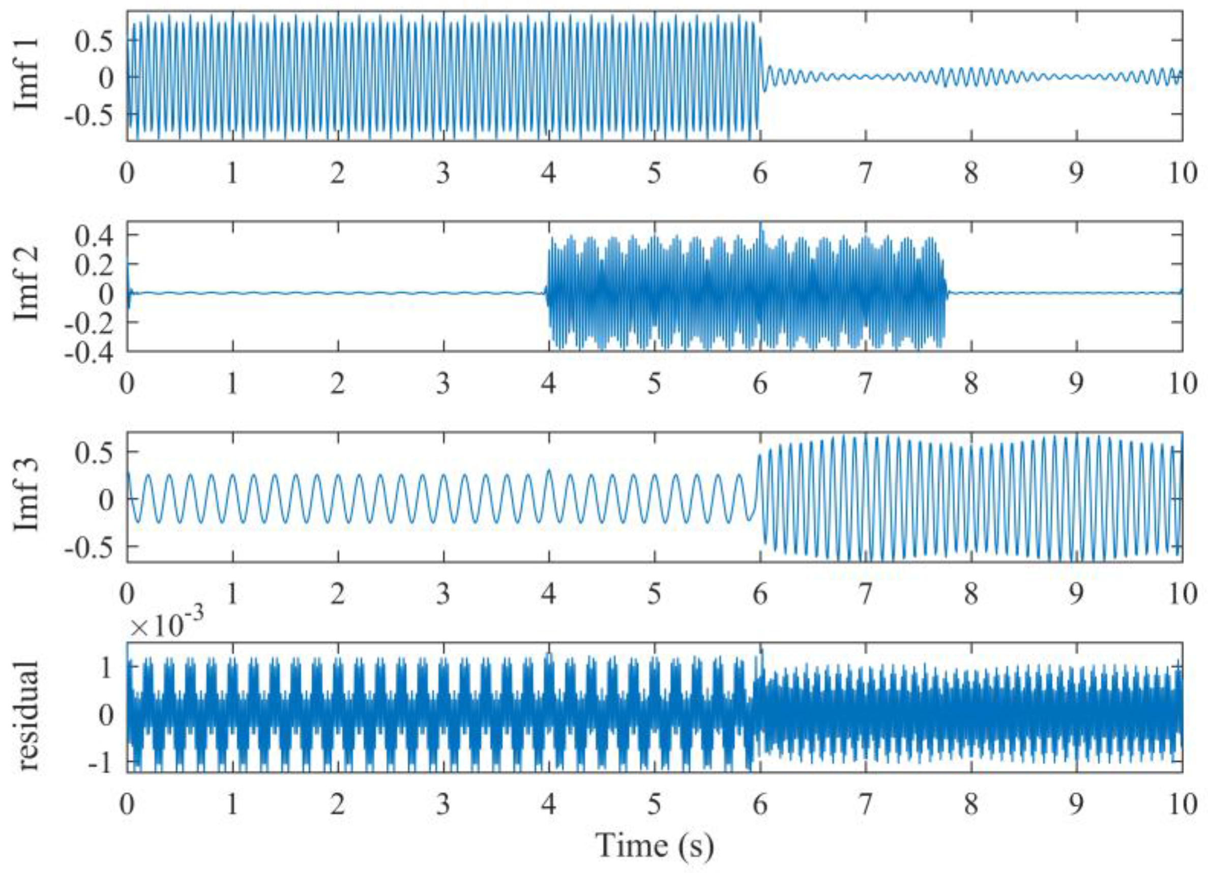
The benchmark signal can be decomposed into a set of IMFs by using both EMD and VMD, as shown in Figure 4 and Figure 5, respectively. It is obvious that the decomposition results using VMD are sparser than those obtained using the EMD method. Additionally, similar vibration modes (with similar time-frequency structures) are always decomposed into different IMFs, which is known as the mode-mixing effect). For example, the third sub-component signal (Figure 2d) is mainly located between 6–10 s and its IF is around 10 Hz. However, the EMD scheme separates them and records them in IMF1 and IMF2, in Figure 4. By contrast, the IMFs derived by the VMD scheme match the benchmark better (see Figure 5). More specifically, in Figure 5, IMF1 refers to Figure 2c, IMF2 refers to Figure 2e, and IMF3 refers to both Figure 2b,d. We remark here that the correspondence can be judged not only by the proximity of frequency ranges, but also by the proximity of amplitude.

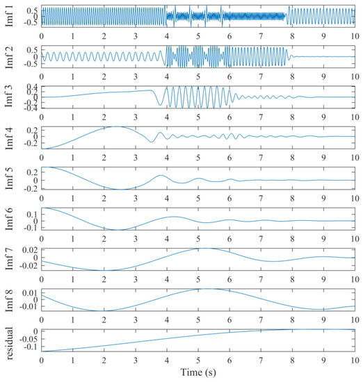
Figure 4. The EMD decomposition results and the residual.

Figure 5. The VMD decomposition results and the residual. IMF1 and IMF2 refer to Figure 2c,e, respectively, and IMF3 refers to both Figure 2b,d.

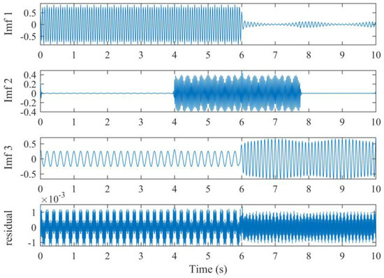
Although there still exist some “mode-mixing” phenomena in the decomposition results by VMD, this defect has been extremely reduced compared with EMD. For example in Figure 5, there are some vibrations with low amplitude or energy remaining at 6~10 s of IMF1, but the sub-component signals (Figure 2d) are mainly reflected in the IMF3. From the above benchmark tests, we observe that the IMFs by VMD are able to reveal the intrinsic properties of the non-stationary signal, whereas EMD may mislead us. Thus, we can draw the conclusion that decomposition by VMD is always more reasonable.

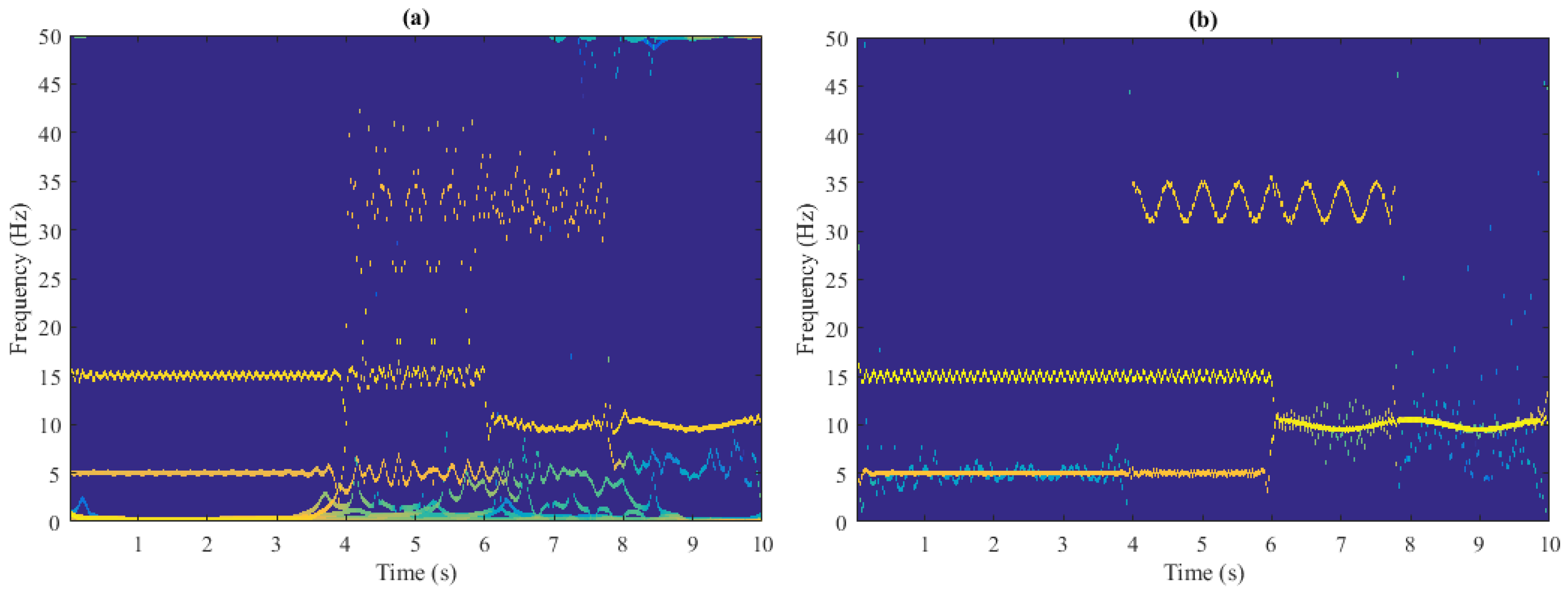
The corresponding IFs can be computed by Taner’s equation using the IMFs decomposed by EMD and VMD. Then the instantaneous spectra can be constructed as shown in Figure 6a,b. Compared with the time-frequency structures in Figure 3, the instantaneous spectrum by VMD is relatively more accurate. This is also because of the fact that VMD decomposition is more reasonable. These synthetic benchmark tests illustrate how the VMD decomposition can be conducted on non-stationary data, avoiding the mode-mixing phenomenon.

Figure 6. The instantaneous spectrum based on (a) EMD and (b) VMD.

3.2. Laboratory Data Tests

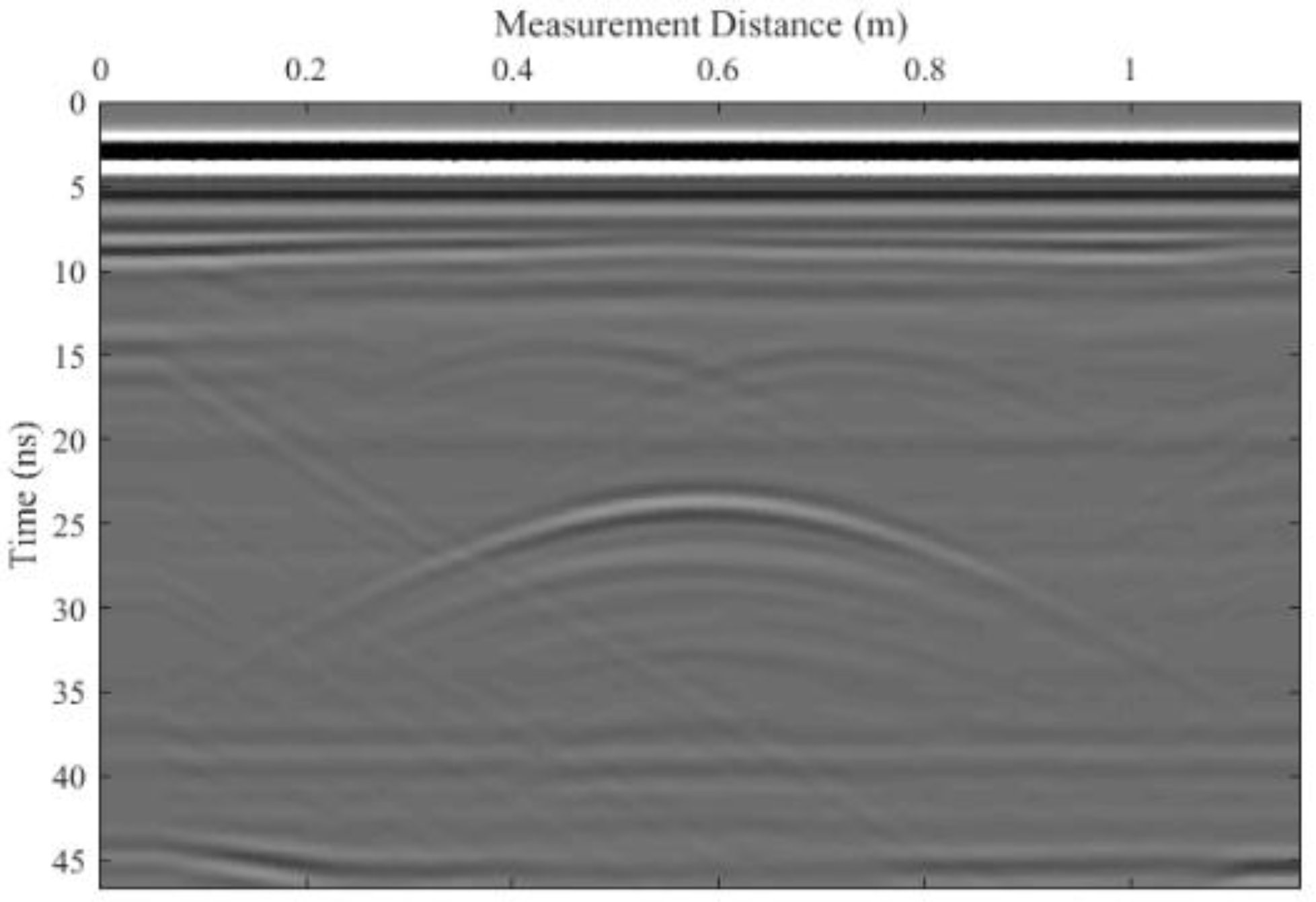
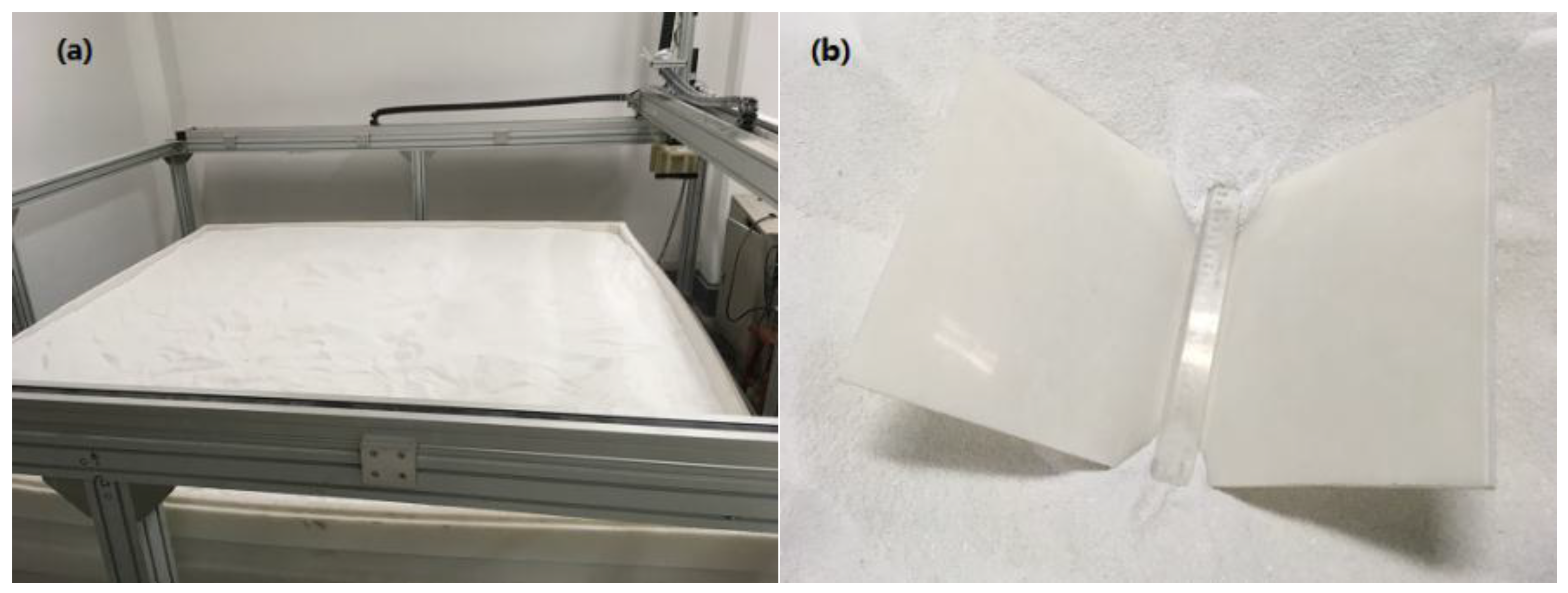
In order to test the VMD method for GPR data decomposition, we employ the laboratory data (shown in Figure 7) for further analysis. The data was collected in a sand trough as shown in Figure 8a, where the target body (Figure 8b) was set at a certain depth.

Figure 7. The laboratory data collected.

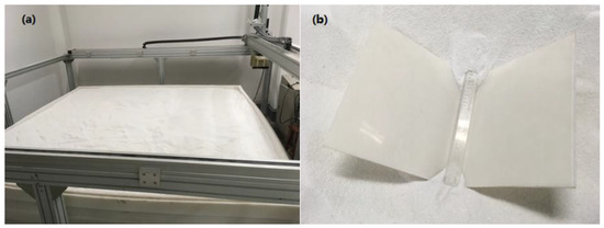
Figure 8. The sand trough (a) and the target body (b).

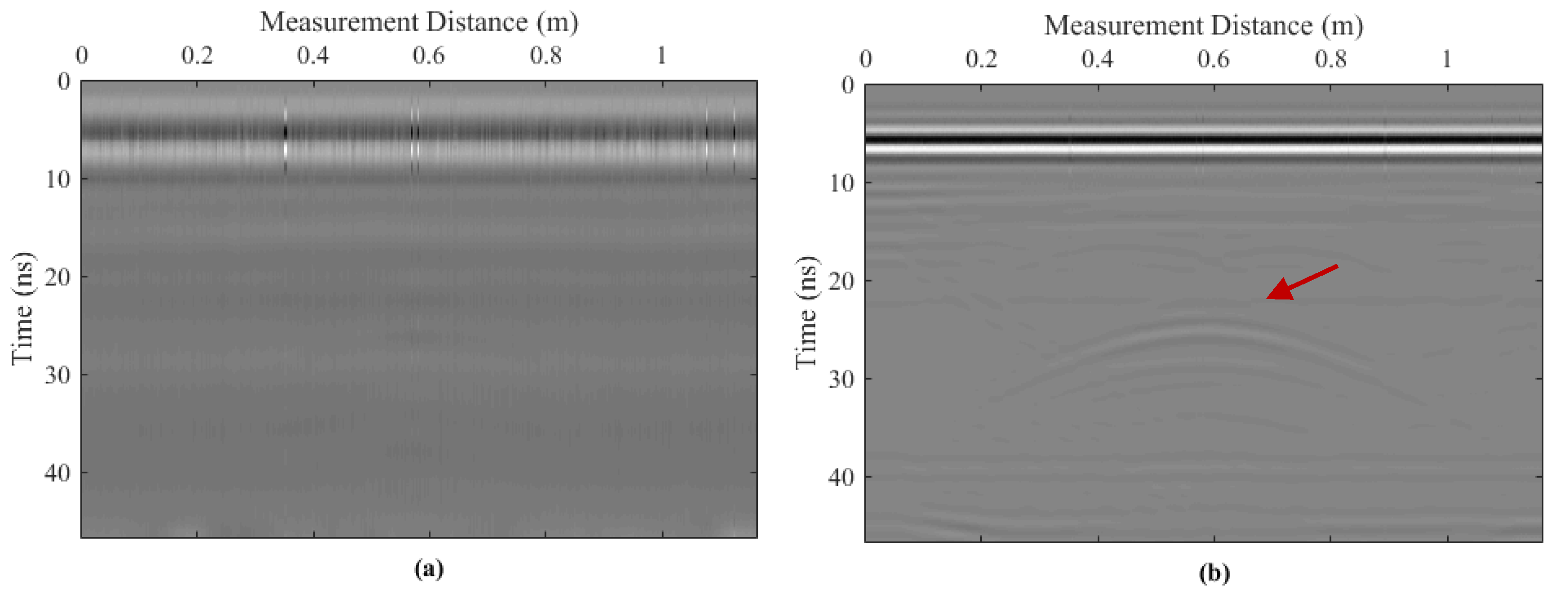
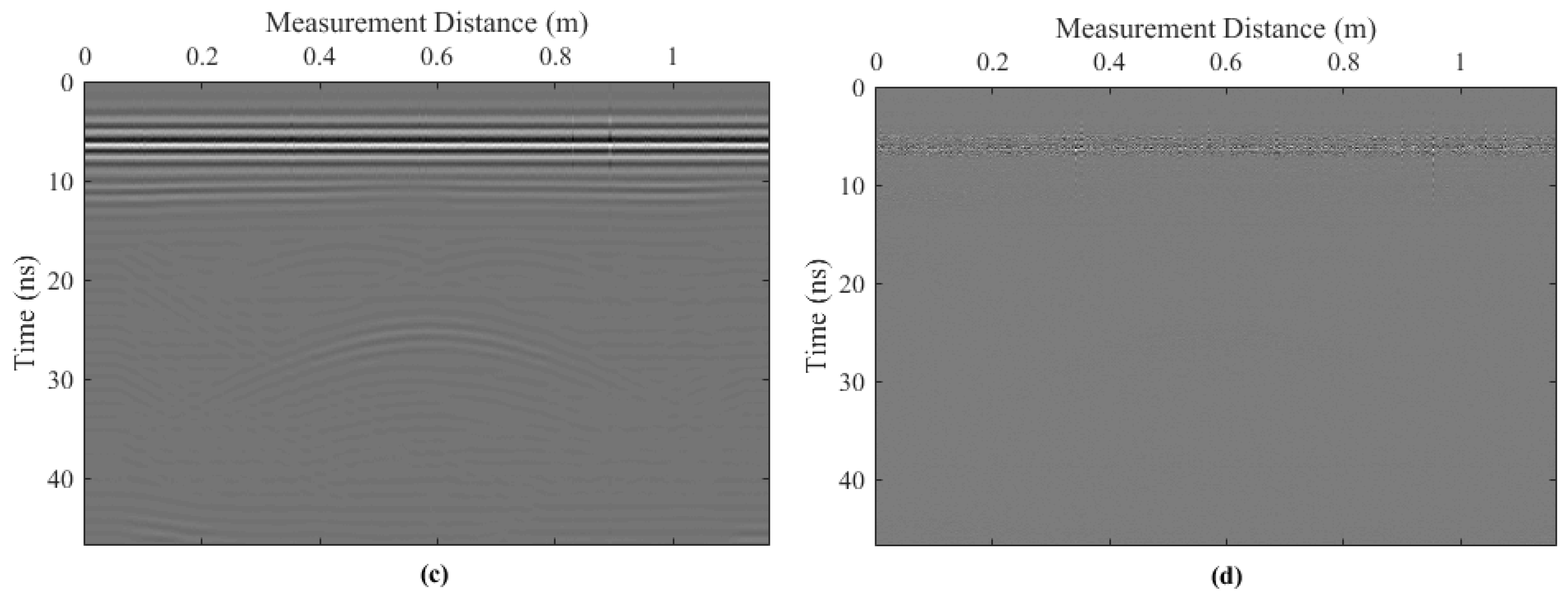
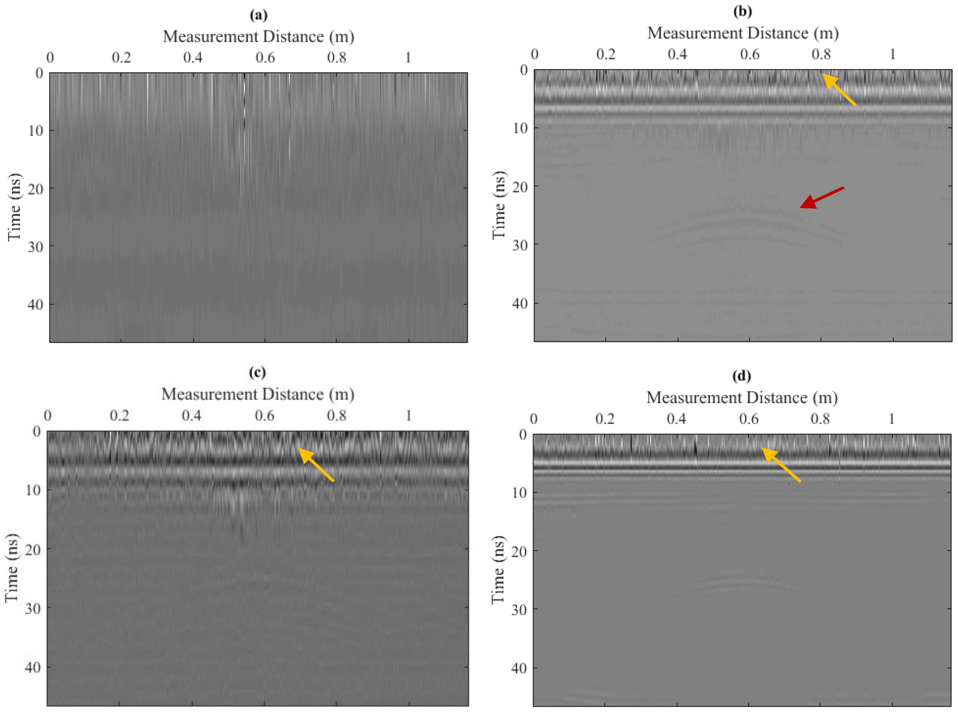
Typically, each trace of the GPR data is non-stationary. We apply the VMD method to decompose the GPR data trace by trace. Then we sort the main components and collect them into several profiles (i.e., the IMF-slices), see Figure 9a–d. For comparison, we adopt a similar way of processing the decomposed IMFs using EMD decomposition, and the generated IMF-slices are shown in Figure 10. In Figure 9, the GPR data are divided into four main components, each of which demonstrates a different vibration mode. The reflection of the buried target is identified in the second IMF-slice by the red arrow pointing to it (see Figure 9b). The noise is shown in Figure 9d, without any important information from the subsurface layers being mixed. In Figure 10, the first IMF-slice is meaningless, and the yellow arrows illustrate the so-called mode-mixing effect. Additionally, the reflection indicated by the red arrow in Figure 10b is not as distinct as that achieved using VMD.

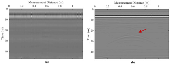
Figure 9. The derived IMF-slices using VMD. (a–d) show the IMF-slice 1–4 respectively.

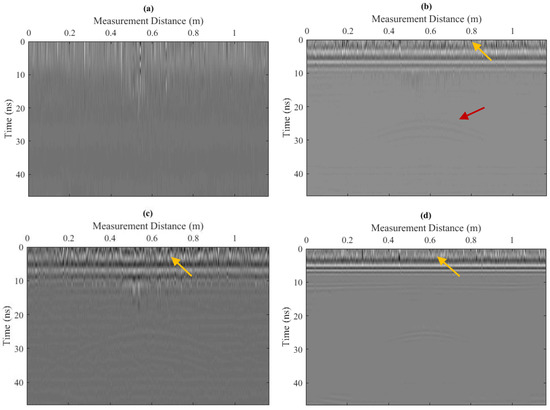
Figure 10. The derived IMF-slices using EMD. (a–d) show the IMF-slice 1–4 respectively.

4. The Use of VMD with Field Dataset

In this section, we use variational mode decomposition to process a field dataset and show the results of the proposed IMF-slices. Subsequently, the corresponding interpretations are drawn.

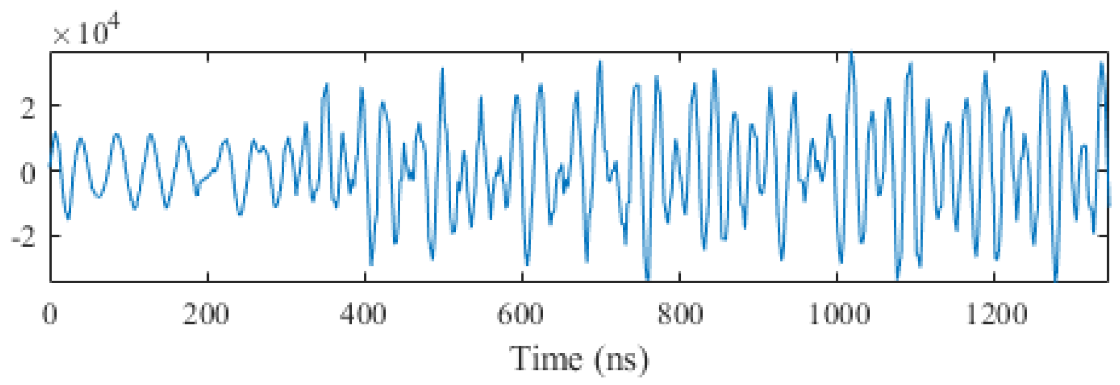
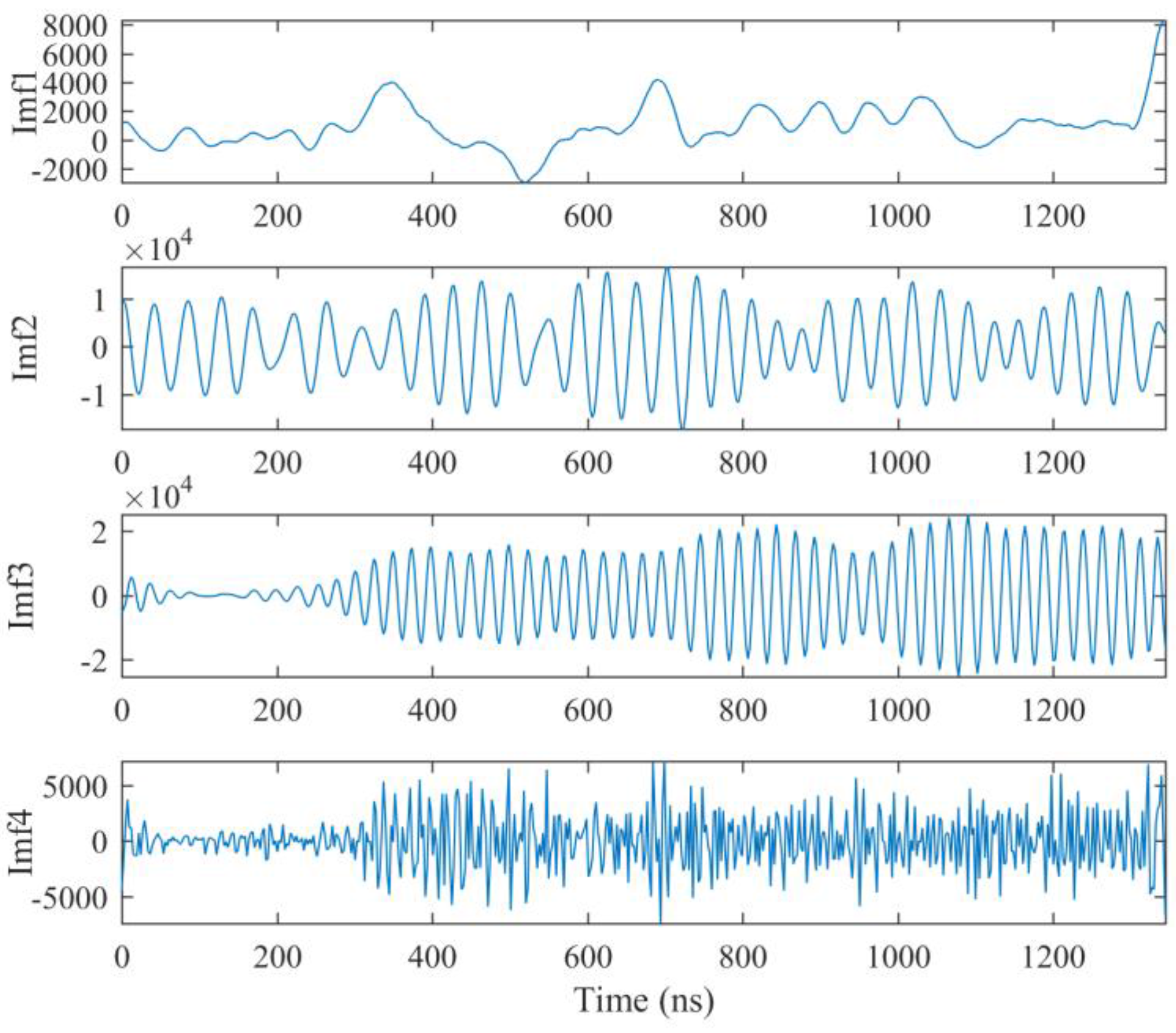
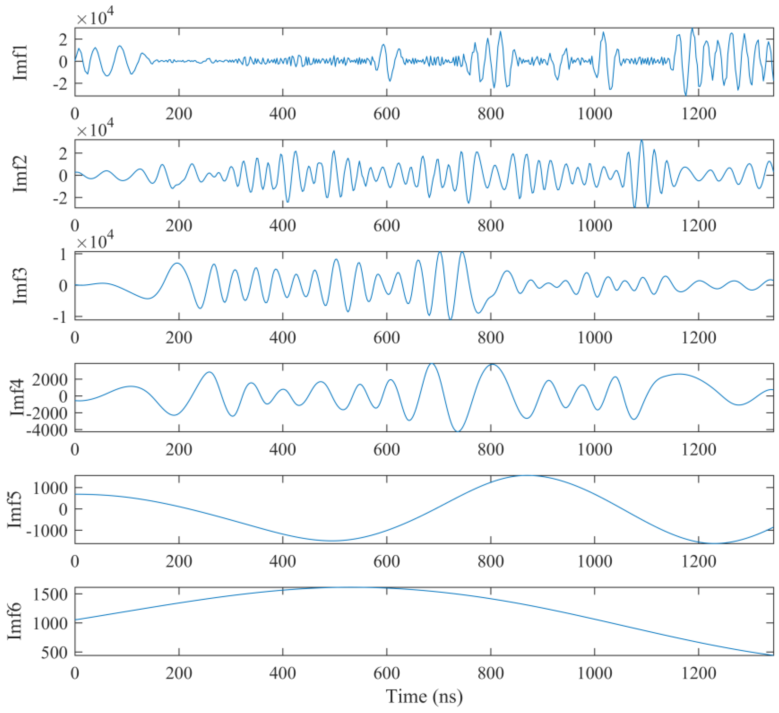
The dataset is shown in Figure 11. It was collected in Yan’an, in the Shanxi Province of China. The data had initially been processed; however, the noise still remains. We firstly use VMD and EMD to decompose one trace respectively (Figure 12), and the decomposed results are shown in Figure 13 and Figure 14, respectively. There are four IMFs generated in Figure 13, of which the first three IMFs are the main components. The fourth IMF can be seen as the noise components. In contrast, the EMD generates more IMFs in Figure 14, and the noise is mixed into the first IMF. In this case, the mode-mixing phenomenon that accompanies EMD decomposition can be lessened by the VMD.

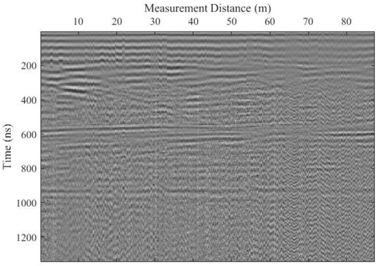
Figure 11. The field GPR dataset.

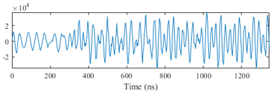
Figure 12. A single trace of the GPR dataset.

Figure 13. The decomposed IMFs using VMD.

Figure 14. The decomposed IMFs using EMD.

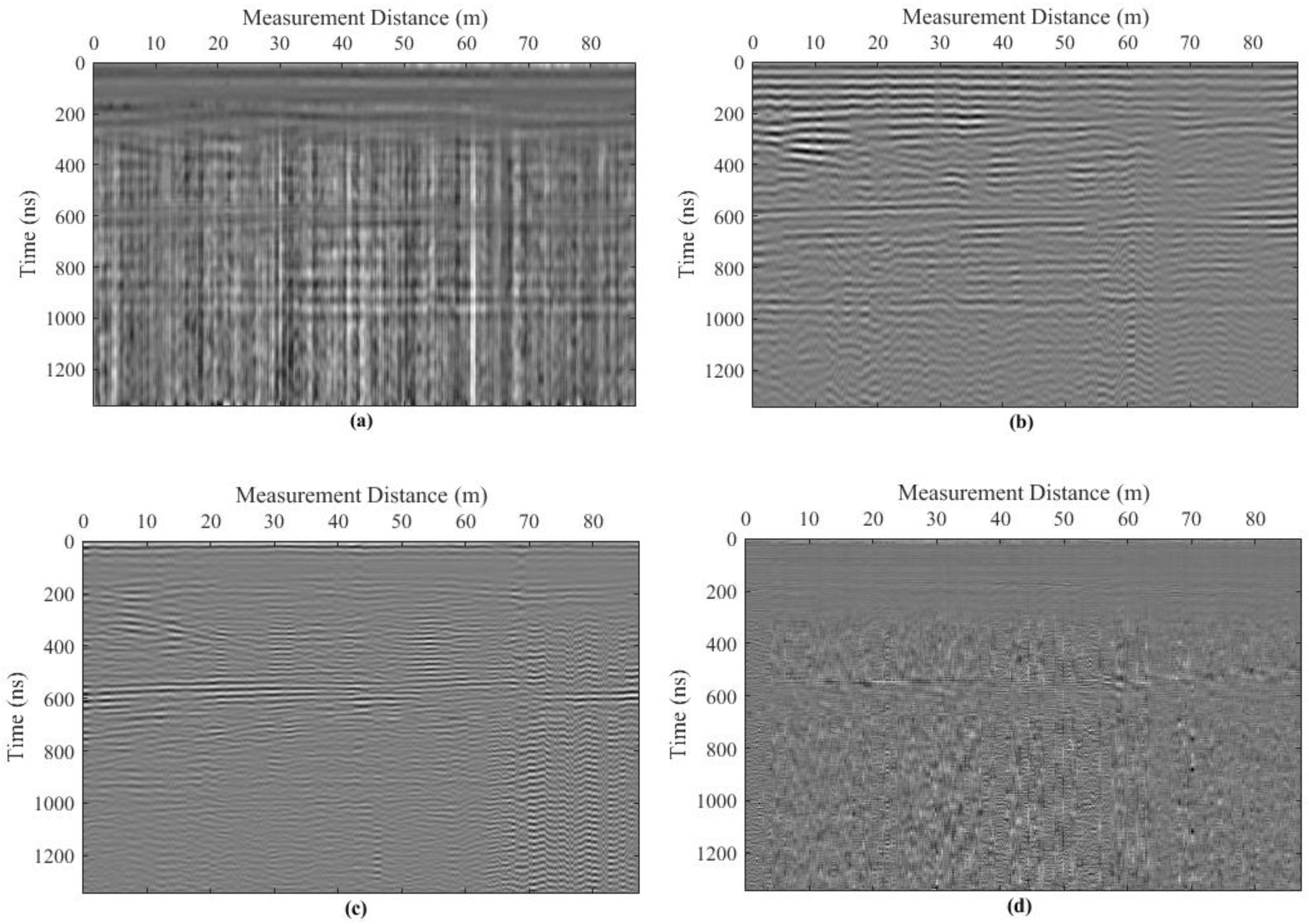
We then compute VMD decomposition for the whole dataset; the derived IMF-slices are shown in Figure 13. The low-frequency components are mainly collected in the first IMF-slice (Figure 15a). We remark here that in this IMF-slice, the DC and the slowly-varying trend term [1] are also collected, so there exists discontinuity of neighboring traces in gray scale. The second and third IMF-slices (Figure 15b–c) demonstrate the subsurface structures at different scales. In the last IMF-slice, the noise of the dataset is extracted, especially in the deep part of the profile.

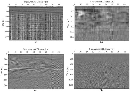
Figure 15. The derived IMF-slices of the field dataset using VMD. (a–d) show the IMF-slice 1–4 respectively.

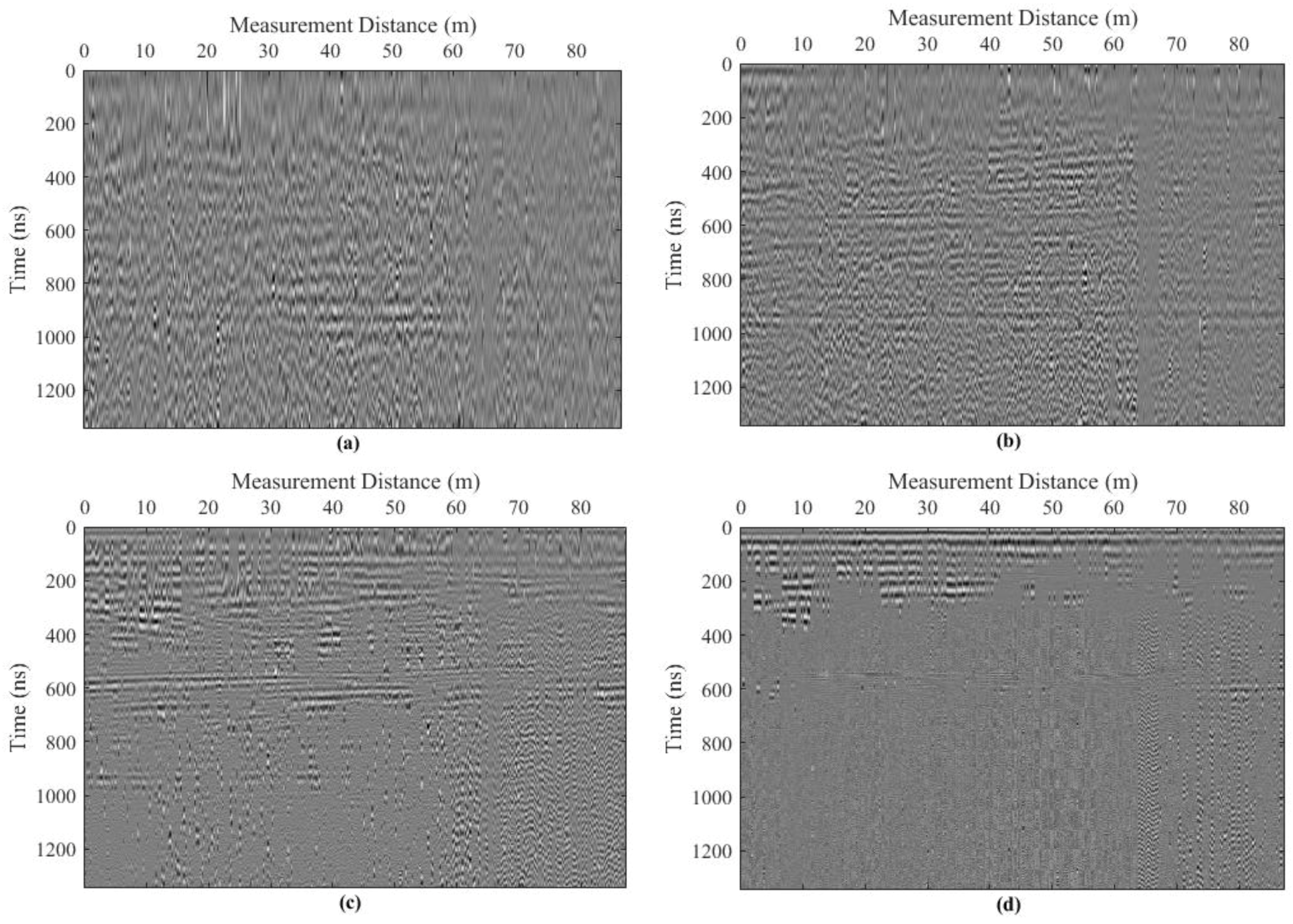
In Figure 16, we also provide comparisons with the IMF-slices based on EMD. In some locations of these IMF-slices, the interpretations are greatly influenced by the mode-mixing of IMFs for different traces. For instance, in Figure 16d the important information in the shallow part and the noise in the deep part are mixed up. It can be observed that, although the IMF-slices by EMD may refer to different frequency ranges, the continuity between neighboring traces is not as good as that achieved with VMD.

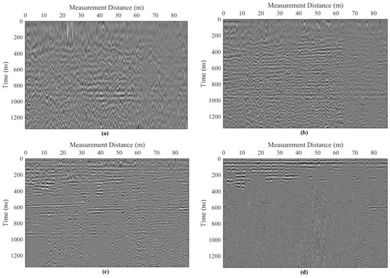
Figure 16. The derived IMF-slices of the field dataset using EMD. (a–d) show the IMF-slice 1–4 respectively.

5. Conclusions

EMD-based methods for GPR imaging provide a novel prospect for interpreting GPR data. Using EMD, the GPR data are decomposed, and the relative stationary IMFs are derived and analyzed for subsequent application. In this paper, variational mode decomposition was introduced. Using VMD, the derived IMFs are sparser and match well with the signal’s intrinsic properties. Based on the decomposition results, the IMFs are sorted and recorded into the proposed IMF-slices for GPR data imaging. We showed its utility on a group of examples, including synthetic benchmark signals, laboratory data and a field dataset. Using IMF-slices, GPR data could be divided into several IMF-slices, each of which delineates a main vibration mode and some subsurface layer and geophysical events can be identified more clearly.

However, the proposed IMF-slices method still requires empirically pre-defined parameters. If the frequency ranges for each IMF-slice are estimated wrongly, or the time-frequency structures of the traces in the GPR profile vary sharply, it is difficult to find a unified standard to separate the different IMF-slices. In our future work, we need to rethink and seek for more intelligent schemes or more automatic procedures for classifying the derived IMFs for the IMF-slices. Additionally, for the accurate detection of the subsurface targets, some figures of merit could also be employed to assess the generated IMF-slices, such as receiver operating characteristics (ROC) [21]. In this case, VMD decomposition may be extended and applied to more aspects for GPR data processing and imaging.

References

- Huang, N.E.; Shen, Z.; Long, S.R.; Wu, M.C.; Shih, H.H.; Zheng, Q.; Yen, N.-C.; Tung, C.C.; Liu, H.H. The empirical mode decomposition and the Hilbert spectrum for nonlinear and non-stationary time series analysis. Proc. R. Soc. Lond. Seri. A Math. Phys. Eng. Sci. 1998, 454, 903–995. [Google Scholar] [CrossRef]
- Rioul, O.; Vetterli, M. Wavelets and signal processing. IEEE Signal Process. Mag. 1991, 8, 14–38. [Google Scholar] [CrossRef]
- Sinha, S.; Routh, P.; Anno, P.; Castagna, J. Spectral Decomposition of Seismic Data with Continuous Wavelet Transform. Geophysics 2005, 70, P19–P25. [Google Scholar] [CrossRef]
- Stockwell, R.G.; Mansinha, L.; Lowe, R.P. Localization of the complex spectrum: The S transform. IEEE Trans. Signal Process. 1996, 44, 998–1001. [Google Scholar] [CrossRef]
- Cheng, Z.; Chen, W.; Chen, Y.; Liu, Y.; Liu, W.; Li, H.; Yang, R. Application of bi-Gaussian S-transform in high-resolution seismic time-frequency analysis. Interpretation 2017, 5, SC1–SC7. [Google Scholar] [CrossRef]
- Feng, X.; Zhang, X.; Liu, C.; Lu, Q. Single-channel and multi-channel orthogonal matching pursuit for seismic trace decomposition. J. Geophys. Eng. 2017, 14, 90–99. [Google Scholar] [CrossRef]
- Zhang, X.; Feng, X.; Liu, C.; Chen, C.; Li, X.; Zhang, Y. Seismic matching pursuit decomposition based on the attenuated Ricker wavelet dictionary. In Proceedings of the 79th EAGE Conference and Exhibition 2017, Paris, France, 12–15 June 2017. [Google Scholar]
- Li, J.; Liu, C.; Zeng, Z.; Chen, L. GPR Signal Denoising and Target Extraction With the CEEMD Method. IEEE Geosci. Remote Sens. Lett. 2015, 12, 1615–1619. [Google Scholar]
- Lu, Q.; Liu, C.; Zeng, Z.; Li, J.; Zhang, X. Detection of human’s motions through a wall using UWB radar. In Proceedings of the 2016 16th International Conference on Ground Penetrating Radar (GPR), Hong Kong, China, 13–16 June 2016; pp. 1–4. [Google Scholar]
- Chen, Y.; Ma, J. Random noise attenuation by f-x empirical-mode decomposition predictive filtering. Geophysics 2014, 79, V81–V91. [Google Scholar] [CrossRef]
- Qin, Y.; Qiao, L.H.; Ren, X.Z.; Wang, Q.F. Using bidimensional empirical mode decomposition method to identification buried objects from GPR B-scan image. In Proceedings of the 2016 16th International Conference on Ground Penetrating Radar (GPR), Hong Kong, China, 13–16 June 2016; pp. 1–5. [Google Scholar]
- Dragomiretskiy, K.; Zosso, D. Variational Mode Decomposition. IEEE Trans. Signal Process. 2014, 62, 531–544. [Google Scholar] [CrossRef]
- Liu, W.; Cao, S.; Chen, Y. Applications of variational mode decomposition in seismic time-frequency analysis. Geophysics 2016, 81, V365–V378. [Google Scholar] [CrossRef]
- Liu, W.; Cao, S.; Wang, Z.; Kong, X.; Chen, Y. Spectral Decomposition for Hydrocarbon Detection Based on VMD and Teager-Kaiser Energy. IEEE Geosci. Remote Sens. Lett. 2017, 14, 539–543. [Google Scholar] [CrossRef]
- Liu, W.; Cao, S.; Wang, Z. Application of variational mode decomposition to seismic random noise reduction. J. Geophys. Eng. 2017, 14, 888–899. [Google Scholar] [CrossRef]
- Boyd, S.; Vandenberghe, L. Convex Optimization; Cambridge University Press: New York, NY, USA, 2004. [Google Scholar]
- Hestenes, M.R. Multiplier and gradient methods. J. Optim. Theory Appl. 1969, 4, 303–320. [Google Scholar] [CrossRef]
- Taner, M.; Koehler, F.; Sheriff, R. Complex seismic trace analysis. Geophysics 1979, 44, 1041–1063. [Google Scholar] [CrossRef]
- Herrera, R.H.; Tary, J.B.; van der Baan, M. Time-frequency representation of microseismic signals using the synchrosqueezing transform. In Proceedings of the GeoConvention 2013, Integration, Calgary, AB, Canada, 6–12 May 2013. [Google Scholar]
- Fomel, S. Seismic data decomposition into spectral components using regularized nonstationary autoregression. Geophysics 2013, 78, O69–O76. [Google Scholar] [CrossRef]
- Rodríguez, A.; Salazar, A.; Vergara, L. Analysis of split-spectrum algorithms in an automatic detection framework. Signal Process. 2012, 92, 2293–2307. [Google Scholar] [CrossRef]
© 2018 by the authors. Licensee MDPI, Basel, Switzerland. This article is an open access article distributed under the terms and conditions of the Creative Commons Attribution (CC BY) license (http://creativecommons.org/licenses/by/4.0/).