A Markovian Approach to Unsupervised Change Detection with Multiresolution and Multimodality SAR Data

Abstract

In the framework of synthetic aperture radar (SAR) systems, current satellite missions make it possible to acquire images at very high and multiple spatial resolutions with short revisit times. This scenario conveys a remarkable potential in applications to, for instance, environmental monitoring and natural disaster recovery. In this context, data fusion and change detection methodologies play major roles. This paper proposes an unsupervised change detection algorithm for the challenging case of multimodal SAR data collected by sensors operating at multiple spatial resolutions. The method is based on Markovian probabilistic graphical models, graph cuts, linear mixtures, generalized Gaussian distributions, Gram–Charlier approximations, maximum likelihood and minimum mean squared error estimation. It benefits from the SAR images acquired at multiple spatial resolutions and with possibly different modalities on the considered acquisition times to generate an output change map at the finest observed resolution. This is accomplished by modeling the statistics of the data at the various spatial scales through appropriate generalized Gaussian distributions and by iteratively estimating a set of virtual images that are defined on the pixel grid at the finest resolution and would be collected if all the sensors could work at that resolution. A Markov random field framework is adopted to address the detection problem by defining an appropriate multimodal energy function that is minimized using graph cuts.

1. Introduction

Multitemporal image analysis represents a powerful source of information in Earth observation, especially in applications to environmental monitoring and disaster management. For example, monitoring the dynamics of desertification and urbanization can be accomplished by taking advantage of automatic change detection methods [1,2]. Analyzing the dramatic effects of flooding, fires, earthquakes and other natural disasters as immediately as possible also benefits from multitemporal image analysis techniques [3]. Therefore, being able to jointly process a pair of images taken at different times plays a major role in this context.

Techniques allowing for the detection of changes from remotely-sensed data have been studied for the last two decades [1]. The usage of either multispectral or radar data has been especially investigated. On the one hand, multispectral and hyperspectral data offer the possibility of operating with multidimensional feature spaces, often granting an effective discrimination between changed and unchanged areas [2,4,5,6,7,8]. On the other hand, this type of data is affected by such factors as illumination, atmospheric conditions and cloud cover. These factors critically influence both the performance and the operational applicability of a change detection technique. Conversely, synthetic aperture radar (SAR) imagery is not sensitive to those factors, allowing for the collection of data at nighttime or in conditions where the cloud cover would make it impossible for an optical sensor to gather any information on the Earth’s surface. However, SAR sensors allow one or a few data features (e.g., one amplitude or intensity with a single-polarization SAR or up to four polarimetric channels with a polarimetric SAR-PolSAR-instrument) to be acquired, and these measurements are affected by speckle, which acts as a multiplicative noise-like phenomenon [9]. These issues often reduce the capability to discriminate changed and unchanged areas as compared to the case of multispectral and hyperspectral imagery [3,10]. Because of the speckle, unsupervised change detection with SAR intensity or amplitude data is often addressed by using image ratioing or log-ratioing. The former consists of dividing, pixel by pixel, the SAR intensity or amplitude collected on the first acquisition time by that acquired on the second acquisition time or vice versa [9]. The latter also applies a logarithm to this pixel-wise ratio. Because of the strict monotonicity of the logarithm, these two multitemporal features essentially convey the same information for change detection purposes. The resulting ratio or log-ratio image is processed to determine whether a pixel represents a changed or an unchanged area on the ground. Approaches alternative to image ratioing include the computation of metrics between local pixel intensity distributions at the two acquisition dates (e.g., the Kullback–Leibler distance) [11,12]. On the contrary, while ratioing and log-ratioing are typical choices for change detection with SAR data, other feature extraction strategies are generally used for change detection with multi- and hyper-spectral imagery, because of the different data and noise statistics. These strategies include image differencing [5], change vector analysis [2], the Reed–Xiaoli (RX) detector and its extensions [6,7] and spectrally-segmented linear predictors [8], among others.

In this framework, the possibility of developing techniques that exploit SAR imagery at multiple spatial resolutions presents a great potential. This potential is also enforced by current missions, such as COSMO-SkyMed, TerraSAR-X, RADARSAT-2, PALSAR-2, Kompsat-5 and Sentinel-1, which provide single- or multi-polarimetric images with multiple spatial resolutions and possibly short revisit times. Taking benefit from the data of current and future missions requires exploiting all the information they bring, hence their multiple spatial resolutions, polarizations or frequencies. In this paper, a novel unsupervised method for the identification of changes in multiresolution and multimodal SAR intensity images is proposed.

Indeed, the current state of the art enumerates only a few examples of approaches addressing the change detection problem with multiresolution/multiscale and multimodal SAR data. A research line that has been explored in this perspective is the joint exploitation of unsupervised change detection techniques together with the application of wavelet transformations [13,14]. Wavelet transforms allow decomposing an input image to obtain a pyramid of new images at progressively coarser spatial scales. Change detection is then applied to this pyramid, either hierarchically, from coarser to finer scales, or jointly, in order to fuse the information captured at the considered scales. However, this is different from the task addressed in this paper. While here the problem of change detection from an input pair of multiresolution images is addressed, techniques based on wavelet decompositions usually take single-resolution imagery as input data and generate multiscale data as an internal process for feature extraction purposes.

In 2005, Bovolo and Bruzzone [15] proposed an approach based on an undecimated stationary wavelet transform (SWT) decomposing the log-ratio image into a set of scale-dependent images characterized by different trade-offs between speckle reduction and preservation of geometrical details. The final change map was obtained through adaptive scale-driven fusion algorithms properly exploiting the wavelet transforms at the different scales. In 2010, Moser and Serpico proposed a method [16] for unsupervised change detection integrating decimated wavelet transforms, Markov random fields (MRFs) for contextual modeling and generalized Gaussian models. The method was evaluated on very high resolution COSMO-SkyMed data. Celik and Ma proposed a method [17] exploiting the robustness against noise of the SWT to obtain a multiscale representation of the ratio image. These multiscale data were segmented with a region-based active contour model for discriminating changed and unchanged regions. Another example was given by [18], where Chabira et al. proposed an unsupervised process for the identification of changes in multitemporal and multichannel SAR images not requiring speckle filtering. The method was based on SWT and linear discriminant analysis. On the one hand, these wavelet-based methods extract multiscale information through the related wavelet decompositions, thus intrinsically introducing contextual information into the change detection process and favoring the preservation of image structures at different spatial scales. On the other hand, all of these techniques were developed for the case of single-resolution and single-modality input SAR data. Hence, they are not applicable per se to input data collected at multiple spatial resolutions, unless case-specific reformulations are introduced.

Regarding approaches not based on wavelet decompositions, Moser et al. presented a method [19] using MRFs for spatial-contextual modeling and graph cuts for the optimization of a suitable energy function defined with the goal of discriminating changed and unchanged areas in multiresolution SAR imagery. In 2014, Dellinger et al. proposed a feature-based approach [20] to detect changes between a pair of either optical or radar images. This method was based on the scale-invariant feature transform (SIFT) and on an a contrario approach. In 2015, the same authors presented the SAR-SIFT algorithm [21], which extended the previous approach to SAR images by introducing a speckle-robust definition of the gradient and by taking into consideration both the detection of keypoints and the computation of local descriptors. However, while [19] addressed the same change detection problem as the present paper, the previous works based on SIFT follow a different approach. They rely on the extraction of local features useful for registering the multiresolution data sources; then, change detection is applied to the registered data and not to input images at different resolutions.

While the literature of change detection algorithms for multiresolution SAR data is scarce, significant effort has been put on the development of change detection methods for multichannel SAR images collected by a PolSAR instrument or at multiple radar frequencies. Methods based on the representation of the backscattered signal through the complex-valued polarimetric sample covariance matrix are common in this framework. On the one hand, this representation is comprehensive in the sense that it characterizes all properties of the backscattered SAR return in terms of both amplitude and phase. On the other hand, in this case as well, the related methods focus on single-resolution data and do not address change detection with SAR imagery associated with multiple spatial resolutions. Furthermore, most of these techniques incorporate local spatial information associated with a neighborhood of each pixel, but do not make use of multiscale information within the change detection process. In [22], Erten et al. proposed a method based on the analytical computation of the mutual information, assumed to be maximal where two images taken at different times were identical. The analytical formulation was derived from the joint density function of multitemporal multichannel images based on their second-order statistics. In 2013, Marino et al. [23] proposed a test for the detection of changes in the internal structure of the covariance matrix. In both [22,23], it was assumed that the covariance matrices associated with each SAR pixel followed complex Wishart distributions and that the input data were at the same resolution. In [24], Liu et al. presented an unsupervised change detection method using heterogeneous clutter models and whose similarity measure was not based on the Wishart distribution. Moreover, in [25], a patch-based change detection method for polarimetric SAR data was proposed, while in [26], Akbari et al. presented an unsupervised method based on the relaxed Wishart distribution for textured change detection analysis. Nielsen et al. proposed a method extending the generalized likelihood ratio test to multitemporal and multifrequency data [27]. In 2016, Akbari et al. proposed a test statistic working with multilook covariance matrix data, whose underlying model was assumed to be the scaled complex Wishart distribution and where the similarity between the covariance matrices was measured through the complex-kind Hotelling–Lawley trace statistic [28].

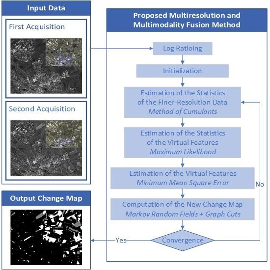
This paper presents a novel algorithm for unsupervised change detection from a multitemporal pair of multiresolution and multimodality SAR images. We assume that the input images are collected over the same geographical area at multiple spatial resolutions at both observation dates and that, for each considered resolution, one or several SAR amplitude channels associated with different modalities (e.g., different polarizations or different frequencies) are acquired. The spatial resolutions and the acquisition modalities are assumed to be the same at both dates, an assumption that is naturally satisfied if the same spaceborne sensors are used for both observations. Log-ratioing is applied to the multitemporal SAR amplitude data of all resolutions and modalities.

The proposed algorithm methodologically comprises MRF modeling [29,30], graph cut minimization [31,32], linear mixtures [33,34], generalized Gaussian distributions [35], Gram–Charlier series expansions [36], maximum likelihood (ML) and minimum mean squared error (MMSE) estimation [37]. It receives, as input, the SAR data collected with all modalities and resolutions and outputs a single change map that takes into account the information gathered by all such sources. The output change map is at the finest among the spatial resolutions of the input multitemporal imagery. This multiresolution and multimodality fusion task is addressed, first, by parametrically modeling the distribution of the data at the different resolutions and by estimating, in the MMSE sense, the “virtual” images that would have been collected in case all modalities worked at the finest resolution. Probability density function (PDF) estimation is accomplished by a case-specific novel approach that combines generalized Gaussians, the Gram–Charlier expansion and a linear mixture model to formulate the ML rule consistently with the multiresolution structure of the input data. This choice makes it possible to benefit from the good properties of ML estimators, such as consistency and asymptotic efficiency, which are well known from the Bayesian estimation theory [38]. Then, the virtual and the finest resolution images are fused in a Markovian framework by defining a novel energy function that is minimized through graph cuts. The MRF formalization based on virtual features is partly inspired by [33,34], in which a similar idea was used to address the classification of optical multispectral images based on Gaussian class-conditional distributions.

The main novel contributions of this paper include: (i) the development of an unsupervised change detection method for the challenging case of an input pair of multiresolution and multimodality SAR images; (ii) the generalization of the MRF modeling with virtual features in [33,34] from the case of multispectral image classification to that of SAR change detection, and the corresponding methodological extension through generalized Gaussian and Gram–Charlier probabilistic models; and (iii) the development of a case-specific ML parameter estimation algorithm for these non-Gaussian models, when combined with the considered multiresolution data structure. We recall that we presented a first preliminary formulation of this approach in the conference paper [19]. On the one hand, the present work and the one in [19] share the idea of addressing multiresolution change detection through virtual features. On the other hand, the method developed here is based on a complete redefinition of the related probabilistic models and parameter estimation strategies (see also Section 3).

We assume that the temporal pair of input images is registered. For the sake of clarity, we shall methodologically describe the proposed technique in the case of a pair of images collected at two distinct spatial resolutions with a single-channel acquisition at each resolution. An example may be the joint use of higher resolution COSMO-SkyMed stripmap data and of lower resolution COSMO-SkyMed ScanSAR data. The extension to other multiresolution SAR data configurations, possibly involving more than two resolution levels and/or multiple polarizations or multiple frequencies for each level, is straightforward and is discussed in a later section.

This paper is organized as follows. The developed methodology is presented in Section 2. First, Section 2.1 proposes the mathematical formulation of the algorithm and presents the required assumptions. Then, the techniques developed for estimating the PDFs of the input and virtual data are reported in Section 2.2, and the estimation of the virtual features is described in Section 2.3, while energy minimization is discussed in Section 2.4. Finally, the extension of the proposed methodology to the general case of more than two resolutions and multiple channels is presented in Section 2.5. Section 3 and Section 4 report the experimental results obtained with COSMO-SkyMed images. The dataset used for experiments is described, experimental results and comparisons reported and an in-depth discussion of the change detection performances presented. Conclusions are drawn in Section 5.

2. Methodology

2.1. Proposed Multiresolution Model and Change Detection Method

2.1.1. Model, Assumptions and Overview of the Method

Let us consider a multitemporal pair of multiresolution and possibly multimodality SAR images. As mentioned in the previous section, we shall describe the methodological formulation of the proposed technique by focusing on the case in which, on each of the two acquisition dates, a finer resolution and a coarser resolution image are available. All such images are assumed to be in SAR amplitude format. For the sake of clarity, first we will consider the case of a single-channel finer resolution image and a single-channel coarser resolution image. Indeed, an assumption implicit in the described input dataset is that the same spatial resolutions and data modalities are observed on both dates, an assumption consistent with the use of the same SAR sensors for both acquisitions.

To address the change detection problem, as a first processing step, image log-ratioing is applied at both resolution levels. Image log-ratioing results in a single-channel log-ratio image at the finer resolution and a single-channel log-ratio image at the coarser resolution. Log-ratioing allows extracting, from the images collected at different dates at each resolution level, a feature that is expected to emphasize the discrimination between changed and unchanged areas. Indeed, log-ratioing transforms the multiplicative speckle into an additive noise-like term. Therefore, if the speckle contributions associated with the same pixel in the observations taken on the two acquisition times are independent, then they contribute additively to noise variance in the log-ratio domain. Hence, the log-ratio image is generally expected to look more noisy than the two individual single-time images on a log scale.

Let $I\subset {\mathbb{Z}}^2$ be the pixel lattice at the finer resolution and $S\subset {\mathbb{Z}}^2$ be the pixel lattice at the coarser resolution. We define $\rho$ to be the linear resolution ratio between the two pixel lattices. We consider here the finer resolution channel and the coarser resolution channel to have an integer resolution ratio and to be coregistered. Hence, ${\rho }^2$ finer resolution pixels are contained in a single coarser resolution pixel. We indicate that the finer resolution pixel $i\in I$ is contained in the coarser resolution pixel $s\in S$ by $i\prec s$ (Figure 1). Moreover, since we are considering the case of single-channel imagery at both resolution levels, both a pixel $i\in I$ at the finer resolution and a pixel $s\in S$ at the coarser resolution are associated with scalar log-ratio data, which are denoted $x_i^{\prime }$ and $x_s$, respectively.

The goal of the method is the generation of a change map at the finest observed resolution. Let $X={\{x_s\}}_{s\in S}$ and $X^{\prime }={\{x_i^{\prime }\}}_{i\in I}$ be the random fields of coarser resolution and finer resolution SAR log-ratios, respectively. We define a random field $Y={\{y_i\}}_{i\in I}$ of change labels on the finer resolution lattice I. The label of each pixel (a) may be binary, with $y_i=1$ and $y_i=0$ indicating “change” and “no-change” respectively, or (b) may possibly take on three values ($y_i=0,1,2$) to also discriminate changes due to a increased or decreased backscattering coefficient. In Case (a), which is the more common in the area of unsupervised change detection, no further assumptions are necessary. On the contrary, in the addressed multiresolution scenario, Case (b) requires the additional assumption that the increase or decrease in the backscattering coefficient appears consistently across the two resolutions and modalities. Should this assumption be violated, the proposed method would still be applicable as in (a) to generate a binary output. Let C be the set of change classes (i.e., $C=\{0,1\}$ in (a) and $C=\{0,1,2\}$ in (b)).

The input to the proposed method consists of observations of both random fields X and $X^{\prime }$ of log-ratios. To take into account the information from both resolutions, we also assume the existence of a further random field of virtual features to be estimated on the basis of the coarser resolution observations. We define a random field $V={\{v_i\}}_{i\in I}$ of virtual features $v_i\in \mathbb{R}$, defined on the finer resolution lattice, but related to the coarser resolution observations through a linear mixture:

$${\displaystyle x_s=\alpha \sum _{i\prec s}{v}_i,\forall s\in S,\alpha ={\rho }^{-2}.}$$

(1)

A similar assumption is used for optical data in [33,34], where Solberg et al. and Moser et al. postulated the existence of a linear mixture relating the observations at coarser resolution with virtual data at finer resolution. Those methods regarded multispectral data, for which unmixing concepts provided an indirect background to this assumption. This paper proposes the adaption of a similar model to the case of multiresolution SAR log-ratio images. For this purpose, the related probabilistic model has been completely reformulated according to the different distribution of the input data (see Section 2.1.2). On the one hand, the linear mixture formulation may bear formal similarities with the multilooking concept, although multilooking is applied in the SAR intensity domain and not in the SAR log-ratio domain. On the other hand, this model assumption is accepted here to favor analytical tractability of the multiresolution fusion process. Moreover, as a further hypothesis, the virtual features $v_i$ are assumed independent and identically distributed (i.i.d.) when conditioned to the labels $y_i$ ($i\in I$). The same i.i.d. assumption is accepted with regard to the distribution of the finer resolution log-ratios $x_i^{\prime }$ when conditioned to the labels $y_i$ ($i\in I$). Such i.i.d. conditions are usually accepted working hypotheses in change detection methods based on Bayesian probabilistic modeling [4].

The change detection problem is solved in a Bayesian framework through the adoption of a Markov model. Markov random fields [29,39,40] are a family of two-dimensional stochastic processes allowing multisource data [41] and contextual information [30,40] to be included in Bayesian image analysis tasks. Through MRF modeling, it is possible to formulate the maximum a posteriori (MAP) decision rule in terms of the minimization of a suitable energy function [29,39].

The energy function of the proposed model is composed of three terms. The first is a pixel-wise contribution related to the distribution of the pixel log-ratios on the finer resolution lattice. The second is another pixel-wise term related to the distribution of the virtual features. The third one brings about local contextual information and is represented by a spatial MRF model [30] for the local neighborhood of each pixel:

$${\displaystyle U(Y\mid X,X^{\prime })={\beta }_1\sum _{i\in I}{D}^{\prime }(x_i^{\prime }\mid y_i)+{\beta }_2\sum _{i\in I}D(v_i\mid y_i)+{\beta }_3\sum _{i\sim j}W(y_i,y_j),}$$

(2)

where ${\beta }_1,{\beta }_2$ and ${\beta }_3$ are weight coefficients, $W(·)$ is the pairwise potential of the MRF model, $D^{\prime }(·)$ and $D(·)$ are unary potentials related to the class-conditional statistics of $x_i^{\prime }$ and $v_i$, respectively, and $i\sim j$ indicates that pixels $i,j\in I$ are neighbors. The first order neighborhood is used, i.e., the neighbors of $i\in I$ are its four adjacent pixels. The two unary potentials are defined according to the PDFs of $x_i^{\prime }$ and $v_i$, conditioned to the label $y_i$ ($i\in I$) and parametrically or semi-parametrically modeled as described in Section 2.1.2. Specifically, $U(Y|X,X^{\prime })$ is the energy associated with the posterior probability distribution of the label random field Y, given the observed random fields X and $X^{\prime }$. As we shall discuss in the next paragraph, the random field V of the virtual features is iteratively estimated as a function of $X^{\prime }$ and Y. Hence, consistent with Bayes’ theorem and with the usual formulation of MRF-based classifiers [29,30], the pairwise potential $W(y_i,y_j)$ is related to the prior distribution of Y, whereas the unary potentials $D(v_i\mid y_i)$ and $D^{\prime }(x_i^{\prime }\mid y_i)$ are related to the conditional PDFs of $x_i^{\prime }$ and $v_i$ given Y.

An overview of the proposed method is reported in Figure 2. The method, after an initialization phase, is iterative and estimates, on each iteration, the conditional PDFs of the finer resolution log-ratios and of the virtual features. The estimated PDFs are incorporated into the unary potentials and used in a minimum energy problem that is solved through graph cuts.

More in detail, the initial change map is obtained by applying the generalized Kittler and Illingworth thresholding (GKIT) algorithm [42] to the coarser resolution input channel. This input is used in the initialization phase because a preliminary detection of changed areas may generally be easier at a coarser than at a finer spatial resolution. The map obtained by GKIT at the coarser resolution is upsampled through nearest-neighbor interpolation to provide the initial change map on the finer resolution pixel lattice. Here, nearest neighbor interpolation is used to make sure that the upsampled map takes again values in the set C of classes. GKIT is an unsupervised Bayesian thresholding technique, in which case-specific parametric models for the statistics of SAR ratio data are integrated. Details on this method can be found in [42].

On each iteration of the proposed method, the current change map is used to estimate the class-conditional PDFs of the finer resolution log-ratio and of the virtual features (see Section 2.2). Then, given again the current change map, an MMSE estimate of the random field V of the virtual features is computed (see Section 2.3). Finally, given the estimated virtual features and class-conditional PDFs, a MAP estimate of the label field Y is obtained by solving the minimum energy problem through graph cuts, thus resulting in an updated change map (see Section 2.4). These steps are iterated until the percentage of pixels whose labels are different in two consecutive iterations goes below a predefined threshold (equal to 0.1% in the experiments of the paper). Therefore, the change map is iteratively used to tune the estimated PDF models and virtual features. At the same time, the label field Y is updated at each iteration based on the observation of the field $X^{\prime }$ (i.e., the finer resolution log-ratio data) and on the estimation of the field V (i.e., the virtual features). Hence, as the proposed method iterates, the evolution of the estimates of the virtual features is determined by the evolution of the change map and vice versa.

2.1.2. PDF Models for Finer-Resolution Log-Ratios and Virtual Features

Regarding the observed pixel intensities, Bruzzone et al. have demonstrated in [43] that the generalized Gaussian (GG) distribution is an accurate model for the statistics of the log-ratio of SAR amplitudes or intensities in changed and unchanged areas. Here, we use this model for the distribution of the log-ratio data on both the finer- and the coarser resolution pixel lattices, when conditioned to the label field. A random variable z is GG-distributed if its PDF is [35]:

$$g(z\mid \mathit{\kappa })=\frac{\lambda \Gamma {(\frac{3}{\lambda })}^{\frac{1}{2}}}{2\sqrt{{\kappa }_2}\Gamma {(\frac{1}{\lambda })}^{\frac{3}{2}}}exp\left[-\frac{\Gamma {(\frac{3}{\lambda })}^{\frac{\lambda }{2}}}{\Gamma {(\frac{1}{\lambda })}^{\frac{\lambda }{2}}}{\left|\frac{z-{\kappa }_1}{\sqrt{{\kappa }_2}}\right|}^{\lambda }\right].$$

(3)

It is characterized by the first-, second- and fourth-order cumulants ${\kappa }_1=E\{z\}$, ${\kappa }_2=\mathrm{Var}\{z\}$ and:

$${\kappa }_4={\mathrm{Cumul}}_4\{z\}=E\{{(z-{\kappa }_1)}^4\}-3{\kappa }_2^2,$$

(4)

which are collected in the parameter vector $\mathit{\kappa }=[{\kappa }_1,{\kappa }_2,{\kappa }_4]$. The shape parameter $\lambda$ ($\lambda >0$) is, in turn, determined univocally by ${\kappa }_2$ and ${\kappa }_4$ through the relation:

$$\gamma =\frac{{\kappa }_4}{{\kappa }_2^2}+3=\frac{\Gamma (\frac{5}{\lambda })\Gamma (\frac{1}{\lambda })}{{\Gamma (\frac{3}{\lambda })}^2},$$

(5)

which is invertible with respect to $\lambda$ and in which $\gamma$ is the normalized excess kurtosis of z [35]. The third-order cumulant is not considered because it vanishes for the GG distribution.

In the proposed method, for each class $c\in C$, a separate GG model $g(·|{\mathit{\kappa }}_c^{\prime })$ with a parameter vector ${\mathit{\kappa }}_c^{\prime }=[{\kappa }_{1c}^{\prime },{\kappa }_{2c}^{\prime },{\kappa }_{4c}^{\prime }]$ is defined for the PDF of the finer resolution log-ratio $x_i^{\prime }$ conditioned to $y_i=c$:

$${\kappa }_{1c}^{\prime }=E\{x_i^{\prime }\mid y_i=c\},{\kappa }_{2c}^{\prime }=\mathrm{Var}\{x_i^{\prime }\mid y_i=c\},{\kappa }_{4c}^{\prime }={\mathrm{Cumul}}_4\{x_i^{\prime }\mid y_i=c\}.$$

(6)

Based on this GG model for the class-conditional statistics of the log-ratio data on the pixel lattice I, the corresponding unary potential is defined as ($i\in I;c\in C$):

$$D^{\prime }(x_i^{\prime }\mid y_i=c)=-lng(x_i^{\prime }\mid {\mathit{\kappa }}_c^{\prime }).$$

(7)

Note that the conditional distribution of $x_i^{\prime }$ given $y_i=c$ does not depend on the pixel location $i\in I$. This is consistent with the aforementioned assumption that the samples of the random field $X^{\prime }$ are i.i.d. when conditioned to the random field Y.

Regarding the PDF of the virtual features, we note that according to Equation (1), if the log-ratios $x_s$ ($s\in S$) on the coarser resolution lattice are GG-distributed when conditioned to the label field Y, then it is not consistent to also model the virtual intensities $v_i$ ($i\in I$) as GG-distributed given Y. Indeed, a linear combination of GG random variables is generally not GG. Nevertheless, a model for the distribution of the virtual features, when conditioned to the label field, is a necessary input to define the corresponding unary potential $D(·)$. The solution proposed here consists of the definition of a new semi-parametric model, where the distribution of the virtual intensities is approximated, in terms of cumulants, through a truncated Gram–Charlier expansion [36].

This expansion provides, under mild assumptions, an asymptotic formulation for a non-Gaussian PDF in terms of a Gaussian term with the same mean and variance and of corrective terms associated with higher-order cumulants and expressed through Hermite polynomials [44]. The Gram–Charlier expansion provides per se an exact formulation of this PDF through a uniformly-convergent series. Truncating this series at a certain order leads to a rather flexible approximation of the PDF based on correcting a Gaussian shape to incorporate skewed, kurtotic, etc., behaviors. This approach has become popular in the literature of the independent component analysis (ICA), as it relates information-theoretic and kurtosis-based formulations of ICA [45]. It is extended here to PDF modeling for multiresolution SAR data fusion. The idea is to adopt a class-conditional distribution defined by such a “perturbed Gaussian”, where the perturbation depends on the cumulants of the virtual features.

For a random variable z with zero mean and unitary variance, the Gram–Charlier approximation $\tilde{p}(z)$ of order n of the PDF of z is constructed as the product [36]:

$$\tilde{p}(z)=\varphi (z)·\sum _{i=0}^n{a}_i{\mathrm{He}}_i(z),$$

(8)

where $\varphi (z)$ is the PDF of the normalized Gaussian distribution $\mathcal{N}(0,1)$, ${\mathrm{He}}_i(z)$ is the Hermite polynomial of order i ($i=0,1,2,\dots$):

$${\mathrm{He}}_i(z)={(-1)}^i{e}^{\frac{z^2}{2}}\frac{d^i}{d{z}^i}(e^{-\frac{z^2}{2}}),$$

(9)

and the coefficients $a_i$ can be related to the cumulants of z. In particular, the fourth-order approximation ($n=4$) can be expressed as [44]:

$$\tilde{p}(z)=\varphi (z)\left[1+\frac{{\kappa }_3}{6}{\mathrm{He}}_3(z)+\frac{{\kappa }_4}{24}{\mathrm{He}}_4(z)\right],$$

(10)

where ${\kappa }_3$ and ${\kappa }_4$ are the third- and fourth-order cumulants of z. If z has zero skewness, then ${\kappa }_3=0$, and the third-order term of Equation (10) vanishes. For a random variable z with generic mean ${\kappa }_1$ and variance ${\kappa }_2$ and with zero skewness, this approximation generalizes as:

$$\tilde{p}(z\mid \mathit{\kappa })=\frac{1}{\sqrt{{\kappa }_2}}\varphi \left(\frac{z-{\kappa }_1}{\sqrt{{\kappa }_2}}\right)\left[1+\frac{{\kappa }_4}{24{\kappa }_2^2}{\mathrm{He}}_4\left(\frac{z-{\kappa }_1}{\sqrt{{\kappa }_2}}\right)\right],$$

(11)

where $\mathit{\kappa }=[{\kappa }_1,{\kappa }_2,{\kappa }_4]$ (as in Equation (3)) and, in particular, ${\mathrm{He}}_4(u)=u^4-6u^2+3$ ($u\in \mathbb{R}$). For additional details on the Gram–Charlier expansion, we refer to [36,44].

In the proposed method, a separate Gram–Charlier approximation $\tilde{p}(·|{\mathit{\kappa }}_c)$ of the form in Equation (11), with a parameter vector ${\mathit{\kappa }}_c=[{\kappa }_{1c},{\kappa }_{2c},{\kappa }_{4c}]$, is introduced for the PDF of the virtual feature $v_i$, given $y_i=c$ ($c\in C;i\in I$):

$${\kappa }_{1c}=E\{v_i\mid y_i=c\},{\kappa }_{2c}=\mathrm{Var}\{v_i\mid y_i=c\},{\kappa }_{4c}={\mathrm{Cumul}}_4\{v_i\mid y_i=c\}.$$

(12)

The zero skewness of this conditional distribution of the virtual features on the finer resolution lattice I is aimed at ensuring consistency with the zero skewness of the conditional GG distribution of the log-ratios on the coarser resolution lattice S. More details on this aspect will be specified in Section 2.2.2. Moreover, in the case of $v_i$, as well, the pixel-wise distribution does not depend on the pixel location because the samples of the random field V are i.i.d. when conditioned to the random field Y.

Based on the described Gram–Charlier model, the corresponding unary potential is defined as ($i\in I;c\in C$):

$$D(v_i\mid y_i=c)=-ln\tilde{p}(v_i\mid {\mathit{\kappa }}_c).$$

(13)

The vectors ${\mathit{\kappa }}_c^{\prime }$ and ${\mathit{\kappa }}_c$ ($c\in C$) parameterize the class-conditional distributions of the observed log-ratios and of the virtual features on the finer resolution lattice, and in turn, the corresponding unary potentials. The following section describes the techniques used to estimate these parameter vectors within the proposed change detection algorithm.

2.2. PDF Parameter Estimation

2.2.1. Estimation of the Class-Conditional PDF of the Log-Ratio at the Finer Resolution

In each iteration of the proposed change detection technique, the method of cumulants is used to estimate the parameters of the GG distribution of $x_i^{\prime }$ conditioned to the current realization of the label random field Y. Estimates ${\widehat{\kappa }}_{1c}^{\prime },{\widehat{\kappa }}_{2c}^{\prime }$ and ${\widehat{\kappa }}_{4c}^{\prime }$ of the cumulants ${\kappa }_{1c}^{\prime },{\kappa }_{2c}^{\prime }$ and ${\kappa }_{4c}^{\prime }$ conditioned to class $c\in C$ are computed as the corresponding sample cumulants (i.e., the sample mean, the sample variance and the fourth-order sample cumulant) of the finer resolution log-ratios over the set of pixels assigned to class c in the current change map.

An estimate ${\widehat{\lambda }}_c$ of the corresponding shape parameter ${\lambda }_c$, to be used in the computation of the GG PDF, is derived through Equation (5) from ${\widehat{\kappa }}_{2c}^{\prime }$ and ${\widehat{\kappa }}_{4c}^{\prime }$. If ${\widehat{\gamma }}_c={\widehat{\kappa }}_{4c}^{\prime }{({\widehat{\kappa }}_{2c}^{\prime })}^{-2}+3$ is the sample normalized excess kurtosis, then in the range ${\widehat{\gamma }}_c\in [1.865,15]$, the inversion of Equation (5) is well approximated as [35]:

$${\widehat{\lambda }}_c=\sqrt{\frac{5}{{\widehat{\gamma }}_c+1.135}}-0.12.$$

(14)

Outside this range, Equation (5) is numerically inverted through Newton’s method. Let ${\widehat{\lambda }}_c=e^{\theta }$. Newton’s procedure is applied with respect to $\theta \in \mathbb{R}$ to avoid an explicit positivity constraint on the shape parameter, and can be expressed as ($n=0,1,2,\dots$):

$${\theta }^{n+1}={\theta }^n-\frac{ln\Gamma (5e^{{\theta }^n})+ln\Gamma (e^{{\theta }^n})-2ln\Gamma (3e^{{\theta }^n})-ln{\widehat{\gamma }}_c}{e^{{\theta }^n}\left[5\Psi (5e^{{\theta }^n})+\Psi (e^{{\theta }^n})-6\Psi (3e^{{\theta }^n})\right]},$$

(15)

where $\Psi (·)$ is the digamma function (i.e., the logarithmic derivative of the Gamma function).

2.2.2. Estimation of the Class-Conditional PDF of the Virtual Features

By definition, the virtual features are not observable (indeed, they are iteratively estimated within the proposed method). Thus, a direct parameter estimation based on the method of cumulants is not possible for their parameter vectors ${\mathit{\kappa }}_c$ ($c\in C$). Here, a case-specific formulation of the ML rule is developed and is applied at each iteration of the proposed change detection method, based on the observed coarser resolution log-ratios and on the current change map. The key idea is that the i.i.d. assumption on the virtual features, given the label field and the linear mixture relation between the virtual features and the coarser resolution log-ratios, allows relating the cumulants of the coarser resolution data to the unknown cumulants of the virtual features. Hence, even though the real class-conditional distribution of the virtual images is unknown, we are able to find a formulation that involves its cumulants, which, in turn, makes it possible to apply the ML criterion.

Specifically, let us collect in the vector ${\mathit{Y}}_s$ all the labels in the finer resolution lattice contained in the coarser resolution pixel $s\in S$, i.e., ${\mathit{Y}}_s={\left[y_i\right]}_{i\prec s}$. Owing to Equation (1) and to the aforementioned i.i.d. assumption, the first-, second- and fourth-order cumulants of $x_s$, given ${\mathit{Y}}_s$, are [37]:

$$\begin{array}{ccc}\hfill K_1({\mathit{Y}}_s,\mathit{\kappa })& =& E\{x_s\mid {\mathit{Y}}_s\}=\alpha \sum _{i\prec s}E\{v_i\mid {\mathit{Y}}_s\}=\alpha \sum _{i\prec s}E\{v_i\mid y_i\}\hfill \\ \hfill K_2({\mathit{Y}}_s,\mathit{\kappa })& =& \mathrm{Var}\{x_s\mid {\mathit{Y}}_s\}={\alpha }^2\sum _{i\prec s}\mathrm{Var}\{v_i\mid {\mathit{Y}}_s\}={\alpha }^2\sum _{i\prec s}\mathrm{Var}\{v_i\mid y_i\}\hfill \\ \hfill K_4({\mathit{Y}}_s,\mathit{\kappa })& =& {\mathrm{Cumul}}_4\{x_s\mid {\mathit{Y}}_s\}={\alpha }^4\sum _{i\prec s}{\mathrm{Cumul}}_4\{v_i\mid {\mathit{Y}}_s\}={\alpha }^4\sum _{i\prec s}{\mathrm{Cumul}}_4\{v_i\mid y_i\},\hfill \end{array}$$

(16)

where $\mathit{\kappa }={\left[{\mathit{\kappa }}_c\right]}_{c\in C}$ collects all parameters of the virtual feature distribution. Let ${\pi }_c({\mathit{Y}}_s)$ be the relative frequency of label $c\in C$ in the portion of the finer resolution lattice that corresponds to coarser resolution pixel $s\in S$, i.e.:

$${\pi }_c({\mathit{Y}}_s)=\frac{1}{{\rho }^2}\sum _{i\prec s}\delta (y_i,c)=\alpha \sum _{i\prec s}\delta (y_i,c),$$

(17)

where $\delta (·)$ is the Kronecker symbol. Hence, Equation (16) simplify to:

$$\begin{array}{ccc}\hfill K_1({\mathit{Y}}_s,\mathit{\kappa })& =& \sum _{c\in C}{\pi }_c({\mathit{Y}}_s){\kappa }_{1c}\hfill \\ \hfill K_2({\mathit{Y}}_s,\mathit{\kappa })& =& \alpha \sum _{c\in C}{\pi }_c({\mathit{Y}}_s){\kappa }_{2c}\hfill \\ \hfill K_4({\mathit{Y}}_s,\mathit{\kappa })& =& {\alpha }^3\sum _{c\in C}{\pi }_c({\mathit{Y}}_s){\kappa }_{4c}.\hfill \end{array}$$

(18)

As discussed in Section 2.1.2, a GG model is assumed for the distribution of the log-ratios, given the label random field, on the coarser resolution lattice, as well. For each pixel $s\in S$ in this lattice, the PDF of $x_s$, conditioned to ${\mathit{Y}}_s$, is GG. In particular, the first-, second- and fourth-order cumulants of this GG PDF are precisely those given by Equation (18). Accordingly, the following log-likelihood function can be defined based on the observed log-ratios on the coarser resolution lattice S and as a function of the unknown parameter vector $\mathit{\kappa }$:

$$L(\mathit{\kappa }\mid X,Y)=\sum _{s\in S}lng\left[x_s\mid K_1({\mathit{Y}}_s,\mathit{\kappa }),K_2({\mathit{Y}}_s,\mathit{\kappa }),K_4({\mathit{Y}}_s,\mathit{\kappa })\right].$$

(19)

To determine an ML estimate $\widehat{\mathit{\kappa }}$, this log-likelihood is maximized with respect to $\mathit{\kappa }$. The maximization is numerically addressed using the BOBYQA (bound optimization by quadratic approximation) algorithm [46]. BOBYQA is an algorithm developed to solve bound constrained optimization problems without using derivatives of the objective function. It solves the problem using a trust region method that approximates the objective function by a quadratic model. Loose bounds are defined for the unknown cumulants (i.e., $\mathit{\kappa }$ is constrained to take values in a multi-dimensional box), and BOBYQA is applied in each iteration of the proposed change detection technique to minimize $L(\mathit{\kappa }\mid X,Y)$, given the observed log-ratio field X on the coarser resolution lattice S and the current change map Y on the finer resolution lattice I.

It is worth noting that, based on the proposed multiresolution model, a sub-optimal solution can be computed in closed form as a starting point for this iterative procedure. Indeed, if a coarser resolution pixel $s\in S$ is pure, i.e., if all the corresponding finer resolution pixels share the same class label c ($y_i=c\forall i\prec s$), then the relative frequencies collapse to ${\pi }_c({\mathit{Y}}_s)=1$ and ${\pi }_b({\mathit{Y}}_s)=0$ for $b\ne c$. Hence, Equation (18) further simplify to:

$$K_1({\mathit{Y}}_s,\mathit{\kappa })={\kappa }_{1c},K_2({\mathit{Y}}_s,\mathit{\kappa })=\alpha {\kappa }_{2c},K_4({\mathit{Y}}_s,\mathit{\kappa })={\alpha }^3{\kappa }_{4c}.$$

(20)

Accordingly, initial estimates of ${\kappa }_{1c}$, ${\kappa }_{2c}$ and ${\kappa }_{4c}$ can be derived from the sample cumulants of the coarser resolution log-ratios of the pure pixels of class c.

Finally, we note that, by analogy with Equation (18), the third-order cumulant of $x_s$, given ${\mathit{Y}}_s$ ($s\in S$), can be written as:

$${\mathrm{Cumul}}_3\{x_s\mid {\mathit{Y}}_s\}={\alpha }^2\sum _{c\in C}{\pi }_c({\mathit{Y}}_s){\kappa }_{3c},$$

(21)

where ${\kappa }_{3c}={\mathrm{Cumul}}_3\{v_i\mid y_i=c\}$ is the third-order cumulant of $v_i$, given $y_i=c$ ($c\in C$). For all coarser resolution pixels $s\in S$, the GG PDF of $x_s$, given ${\mathit{Y}}_s$, has zero skewness, i.e., ${\mathrm{Cumul}}_3\{x_s\mid {\mathit{Y}}_s\}=0$. As the relative frequencies ${\pi }_c({\mathit{Y}}_s)$ are non-negative, this generally implies ${\kappa }_{3c}=0$ for all $c\in C$. Hence, as anticipated in Section 2.1.2, this comment confirms that the choice of modeling the PDF of $v_i$, given $y_i=c$, through a Gram–Charlier approximation with zero skewness is aimed at ensuring consistency with the conditional GG PDF of the coarser resolution data.

2.3. Virtual Feature Estimation

The MMSE estimate of the virtual feature $v_i$ of the pixel $i\in I$ at the finer resolution, given the corresponding observed SAR log-ratio $x_s$ at the coarser resolution $(s\in S,i\prec s)$ and the change labels, is given by [37]:

$${\widehat{v}}_i=E\{v_i\mid {\mathit{Y}}_s\}+\frac{\mathrm{Cov}\{v_i,x_s\mid {\mathit{Y}}_s\}}{\mathrm{Var}\{x_s\mid {\mathit{Y}}_s\}}\left[x_s-E\{x_s\mid {\mathit{Y}}_s\}\right],$$

(22)

where $\mathrm{Cov}\{·\}$ indicates the covariance between a pair of random variables. Substituting the quantities defined above and computing $\mathrm{Cov}\{v_i,x_s|{\mathit{Y}}_s\}$ through Equation (1) leads to:

$${\widehat{v}}_i={\kappa }_{1y_i}+\frac{\alpha {\kappa }_{2y_i}}{K_2({\mathit{Y}}_s,\mathit{\kappa })}\left[x_s-K_1({\mathit{Y}}_s,\mathit{\kappa })\right].$$

(23)

In Equation (23), ${\kappa }_{1y_i}$ and ${\kappa }_{2y_i}$ are the first- and second-order cumulants of $v_i$ conditioned to the label of pixel i (i.e., the pixel where the virtual intensity is being estimated).

In each iteration of the proposed method, after the ML estimate $\widehat{\mathit{\kappa }}$ of $\mathit{\kappa }$ has been computed as described in the previous section, $\widehat{\mathit{\kappa }}$ is plugged into Equation (23), and the estimated virtual feature ${\widehat{v}}_i$ is determined on each pixel $i\in I$ of the finer resolution lattice. This estimate is a function of the coarser resolution observation corresponding to that virtual pixel and of the change map of the current iteration. Thus, the virtual feature field V evolves with the field Y of the change labels. In particular, the virtual features, representing the components of the linear mixture model, estimate how the coarser resolution image would have been if it were acquired at the finer spatial resolution, given the current change map.

2.4. Energy Minimization

Several techniques have been developed in the last few decades for the minimization of a Markovian energy function [30], ranging from deterministic methods like iterated conditional mode (ICM) [47] to stochastic methods like simulated annealing [29]. A major difference between these two approaches resides in the trade-off between computational complexity and optimality of the solution. ICM reaches convergence much faster to a local minimum that is generally biased by the initialization [30,41]. Simulated annealing converges, under suitable assumptions, to the global energy minimum, but generally requires a very long time [29,39].

Graph cut approaches have gained popularity in the last decade and are based on the reformulation of the energy minimization problem as a max-flow/min-cut problem over a suitable graph [48]. In the case of binary classification, they allow a global minimum to be reached in polynomial time [48]. With more than two classes, graph cuts converge to a local minimum characterized by “strong” analytical properties with respect to suitable optimality criteria [31,32,49].

In each iteration of the proposed change detection method, a graph cut approach is used to minimize the energy in Equation (2). If a binary change map is sought for (i.e., if $C=\{0,1\}$), then the globally optimum max-flow/min-cut formulation is used. If three change classes are considered, as discussed in Section 2.1.1 (i.e., if $C=\{0,1,2\}$), then the swap-move technique is used. It expresses a multiclass energy-minimization problem as a sequence of two-class subproblems. For each subproblem, a global energy minimum is reached through the max-flow/min-cut formulation. For the overall swap-move iterative procedure, the resulting solution is proven to satisfy the aforementioned strong local optimality properties and is usually obtained with a short convergence time [31].

The energy in Equation (2) is parameterized by the weight coefficients ${\beta }_1$, ${\beta }_2$ and ${\beta }_3$, whose values have to be determined prior to minimization. First, the weight coefficients ${\beta }_1$ and ${\beta }_2$ are chosen so as to equalize the contributions of the unary potentials included in the energy. The reason is two-fold. First, the proposed method aims at favoring the fusion of the available SAR resolutions and modalities with similar weights into the output change detection result. Second, the unary potential associated with the finer resolution log-ratios is based on a GG PDF, while the unary potential associated with the virtual features is obtained through a Gram–Charlier formulation, which provides an approximation to a PDF, but is not a PDF in a strict sense. In the language of density estimation, the Gram–Charlier approximation would not be a bona fide PDF estimate, e.g., its area is generally not unitary. This may cause unbalancing between the unary potentials in the formulation of the energy function without a proper choice of the weights. Hence, ${\beta }_1$ and ${\beta }_2$ are chosen to be the inverse of the average energy terms they are associated with, i.e.:

$${\beta }_1={\left|{\displaystyle \frac{1}{\left|I\right|·\left|C\right|}\sum _{i\in I}\sum _{c\in C}{D}^{\prime }(x_i^{\prime }\mid y_i=c)}\right|}^{-1},{\beta }_2={\left|{\displaystyle \frac{1}{\left|I\right|·\left|C\right|}\sum _{i\in I}\sum _{c\in C}D(v_i\mid y_i=c)}\right|}^{-1},$$

(24)

where $\left|I\right|$ and $\left|C\right|$ denote the cardinalities of I and C, respectively (i.e., the numbers of finer resolution pixels and of change classes, respectively).

The coefficient ${\beta }_3$ is optimized through Besag’s pseudo-likelihood method [50,51], in which the joint prior distribution of all the labels in the MRF is approximated by the product of the distributions of the labels of the individual pixels, each conditioned to its own neighborhood. It is easy to prove that Besag’s pseudo-likelihood method determines ${\beta }_3$ based on the following maximization problem [10,50]:

$${\beta }_3=\underset{\beta >0}{arg\; max}\sum _{i\in I}\left[\beta m_i(y_i)-ln\sum _{c\in C}{e}^{\beta m_i(c)}\right],\mathrm{where}:m_i(c)=-\sum _{j:i\sim j}W(c,y_j).$$

(25)

For example, if the adopted spatial MRF is the well-known Potts model (i.e., if $W(c,c^{\prime })=-\delta (c,c^{\prime })$ for $c,c^{\prime }\in C$), then $m_i(c)$ represents the number of pixels that belong to the neighborhood of pixel $i\in I$ and are assigned to class $c\in C$. The maximization in Equation (25) can be easily accomplished by Newton–Raphson’s algorithm.

We note that the values of ${\beta }_1,{\beta }_2$, and ${\beta }_3$ are optimized and updated on each iteration of the proposed change detection method, prior to the corresponding application of graph cuts. Therefore, the weight parameters of the MRF model are adaptively tuned in accordance with the evolution of the change map and of the virtual features along the iterations of the method.

2.5. Extension to More Than Two Resolutions and to Multichannel Data

As introduced in Section 2.1.1, the proposed change detection method has been described in detail for the case of input data at two different resolutions, each endowed with a single log-ratio channel. Here, the method is generalized to the case where more than two resolutions are taken into account, and where the number of input channels can be greater than one for each resolution level. These multiple channels correspond to the log-ratio images derived from different SAR modalities, e.g., different polarizations and/or frequencies.

Let us consider the case of SAR log-ratio data at R different resolutions. The log-ratio image at the finest resolution is composed of $N_1$ channels, while the log-ratio image at the r-th coarser resolution is composed of $N_r$ channels, with $r=2,3,\dots ,R$. The change map is computed, as before, at the finest resolution available in the input multiresolution dataset. To fuse the available SAR data into the same framework, the existence of a set of virtual images, again defined on the pixel lattice I at the finest resolution, is postulated. In particular, there is a (scalar-valued) virtual image for each channel of each coarser resolution level. The linear mixture hypothesis is still assumed, the only difference being in the resolution ratio. Given R resolutions, there are $(R-1)$ resolution ratios and corresponding coefficients ${\alpha }_r$, and the linear mixture is formulated as:

$$x_{rns}={\alpha }_r\sum _{i\prec s}{v}_{rni},$$

(26)

where $x_{rns}$ is the intensity of pixel s in the n-th channel of the r-th coarser resolution log-ratio image and $v_{rni}$ is the virtual feature associated with the same channel and resolution level and with pixel $i\prec s$ in the finest resolution lattice ($r=2,3,\dots ,R;n=1,2,\dots ,N_r$).

The MRF energy in Equation (2) is also generalized by extending the GG model to the conditional statistics of all finest resolution log-ratio channels and the Gram–Charlier approximation to the conditional statistics of all virtual features:

$$U(Y\mid X,X^{\prime })=\sum _{i\in I}\left[-\sum _{n=1}^{N_1}{\beta }_{1n}lng(x_{ni}^{\prime }\mid {\mathit{\kappa }}_{n{y}_i}^{\prime })-\sum _{r=2}^R\sum _{n=1}^{N_r}{\beta }_{2rn}ln\tilde{p}(v_{rni}\mid {\mathit{\kappa }}_{rn{y}_i})\right]+{\beta }_3\sum _{i\sim j}W(y_i,y_j),$$

(27)

where $x_{ni}^{\prime }$ is the log-ratio in the n-th channel of pixel $i\in I$ at the finest resolution, ${\mathit{\kappa }}_{nc}^{\prime }$ is the parameter vector of its GG distribution conditioned to $y_i=c$ ($n=1,2,\dots ,N_1;c\in C$), ${\mathit{\kappa }}_{rnc}$ is the parameter vector of the Gram–Charlier model for the PDF of the virtual feature $v_{rni}$ conditioned to $y_i=c$ ($r=2,3,\dots ,R;n=1,2,\dots ,N_r;c\in C$) and ${\beta }_{1n},{\beta }_{2rn}$ and ${\beta }_3$ are weight parameters.

In each iteration of the proposed change detection method, the algorithms described in Section 2.2.1 and Section 2.2.2 are applied separately for each resolution level r and each channel n to estimate the parameter vectors ${\mathit{\kappa }}_{nc}^{\prime }$ and ${\mathit{\kappa }}_{rnc}$ ($c\in C$) of the corresponding conditional GG and Gram–Charlier models. The procedure for the MMSE estimation of the virtual features described in Section 2.3 is applied for each resolution $r\ge 2$ and each channel n separately. The procedure to optimize the weight parameters is extended analogously. Finally, $U(Y\mid X,X^{\prime })$ is minimized with respect to Y through graph cuts as discussed in Section 2.4.

3. Experimental Results

3.1. Dataset and Experimental Setup

A temporal pair of COSMO-SkyMed images, acquired over Amiens, France, was used to validate the proposed method. On each acquisition time, a multiresolution and multimodality SAR dataset was composed of a stripmap image at finer resolution (see Figure 3a,c) and a pair of polarimetric channels at coarser resolution (HH and VV polarizations; see Figure 3b,d, in which the RGB false color composition is such that $\mathrm{R}=\mathrm{G}=\mathrm{HH}$ and $\mathrm{B}=\mathrm{VV}$). Each stripmap image was composed of $1460\times 1140$ pixels captured at a resolution of 5 m, while the polarimetric channels were composed of $365\times 285$ pixels at a resolution of 20 m. The acquisition dates were 28 March and 18 July 2011, for the stripmap images, and 2 April and 23 July 2011, for the polarimetric images. The first stripmap and polarimetric acquisitions were temporally separated by five days, and the second stripmap and polarimetric acquisitions were four days apart. These temporal gaps were much shorter than the almost four months from the first to the second pairs of acquisitions and were consequently neglected. The available configuration yields a resolution ratio $\rho =4$.

First, a comparative analysis was carried out between the results obtained by applying the proposed multiresolution and multimodality change detection method to this dataset and the results obtained by applying the algorithm in a single-resolution and single-modality fashion to the single-channel stripmap images and to the two-channel polarimetric images, separately. In the former case, an MRF energy as in Equation (2), but without the unary term associated with the virtual features was used. The same PDF estimation approach as in Section 2.2.1 was applied in this case, as well. In the case of the application to the polarimetric image pair, the coarser resolution channels were upsampled, and the same method described for the stripmap temporal pair was applied. These comparisons were aimed at evaluating the multiresolution and multimodality fusion capabilities of the proposed approach.

Then, to investigate the role of the virtual features in the proposed method, we evaluated the accuracy that could be obtained when they were replaced by the coarser resolution channels interpolated onto the finer resolution lattice. First, the polarimetric channels collected on each acquisition time were upsampled to the finer resolution lattice and stacked together with the related stripmap channel. Second, the corresponding log-ratios were computed for all these channels on the stripmap lattice. Third, the polarimetric log-ratios were plugged into Equation (2) instead of the virtual features, and their class-conditional PDFs were modeled as generalized Gaussians as in the case of the stripmap log-ratio. Finally, the resulting energy was minimized using graph cuts, and the results were compared to those obtained by the proposed method. This comparison was aimed at analyzing the importance of the virtual features for multiresolution modeling within the proposed technique.

An experimental comparison with the previous algorithm in [10] was also performed through a similar approach, i.e., upsampling the polarimetric temporal pair to the stripmap pixel lattice, ratioing it, stacking it together with the stripmap log-ratio and applying the method in [10] to the resulting stacked dataset. This previous SAR change detection technique is based on a single-resolution MRF in which amplitude ratio channels coming from different sources are fused in the unary term, and PDF estimation and energy minimization are addressed by combining a mode-field approximation of the expectation-maximization (EM) algorithm [52] and the method of log-cumulants. The method can be applied with three parametric models for the class-conditional PDFs, i.e., the log-normal, Nakagami-ratio and Weibull-ratio distributions [10]. Here, all such models have been considered in the experiments. The upsampling and stacking operations allowed comparing the proposed method with a previous approach that supports the detection of changes from multimodality SAR data, but operates at a single spatial resolution. In all experiments and comparisons using MRFs, the Potts model was used.

Finally, comparisons were carried out between the performances of the proposed technique and those obtained by the previous methods in [15,27]. Both these methods, like that in [10], were not developed to deal with input multiresolution SAR data and were consequently extended and adapted to this type of input imagery. These two experiments were aimed at assessing the performances of the proposed technique in comparison with previous unsupervised SAR change detection algorithms based on different methodological key ideas, namely wavelets and likelihood ratio tests (LRT).

Specifically, the “fusion at the decision level on all reliable scales” (FDL-ARS) method in [15] is based on a multiscale SWT of the input single-resolution log-ratio image and on the selection of the optimal scale of decomposition for each pixel. This approach is aimed at minimizing the impact of noise while preserving the geometrical properties of the scene. A separate change map is computed for each scale, and the final result is obtained by a pooling strategy. To adapt this algorithm to the application to the considered multiresolution dataset, we applied it to the stripmap and to the polarimetric log-ratios separately. The SWT was computed so that the coarser resolution polarimetric log-ratios corresponded to the same pixel lattice and spatial resolution as the second level of decomposition of the stripmap log-ratio (because $\rho =4$). Then, the voting procedure was applied to the results obtained on the whole dataset. For each pixel, the pool consisted of the change labels in the maps computed at the various scales up to the optimal scale for that pixel. Majority voting within this pool determined the output label of the pixel. Further details on the method and on the generation of the individual change maps can be found in [15].

The method in [27] was originally developed for single-resolution PolSAR data and formulated in terms of the complex-valued polarimetric sample covariance matrix. For change detection purposes, an LRT for the equality of two complex covariance matrices was derived. Hence, a new feature, corresponding to a metric between two matrix distributions, was computed and thresholded to determine the output change map. Here, the available dataset was in SAR amplitude format; hence, a case-specific (diagonal) formulation of the related covariance matrices was used. To make the method applicable to the considered multiresolution dataset, the polarimetric channels were again upsampled to the pixel lattice of the stripmap data. Receiver operating characteristic (ROC) curves were used to characterize the performance of the method in a threshold-independent way. The method in [27] per se is non-contextual. Therefore, to favor a fair comparison with the proposed technique, which is contextual, it was applied not only to the original dataset, but also after despeckling. A $7\times 7$ and a $15\times 15$ GammaMAP filter [9] was used for this purpose.

3.2. Results and Performances

The considered dataset included two types of change, due to the evolution of the agricultural crops in the imaged area and associated with an increase and a decrease in the backscattering coefficient, respectively. A preliminary visual inspection of the multitemporal images pointed out that the finer resolution stripmap data were poorly informative for the discrimination of one of the two types of change, while both changes were apparent in the polarimetric image pair, yet with obviously coarser spatial detail. This is confirmed by a visual analysis of the log-ratio images (see Figure 3e,f, in which the polarimetric log-ratios are shown in RGB false colors with $\mathrm{R}=\mathrm{G}=$ log ratio of the HH channels and $\mathrm{B}=$ log ratio of the VV channels). On the one hand, “no-change” pixels are expected to exhibit similar amplitudes in the two acquisitions, hence near-zero log-ratios. On the other hand, pixels associated with either type of change are expected to exhibit significantly different amplitudes in the two acquisitions, i.e., log-ratio values that are significantly greater or lower than zero. The grayscale representation of this range of values includes whitish and blackish pixels in the case of significantly positive and negative log-ratios, respectively, and greyish pixels in the case of near-zero log-ratios.

As described in Section 2.1.1, an initialization map was obtained by applying the GKIT algorithm to one of the two polarimetric log-ratio channels. The choice of the channel to use for initialization had no effect on the result, as the initialization maps obtained by applying GKIT to each of the two polarimetric channels differed only in little details. The resulting change map is shown in Figure 4a, together with the result of the first iteration of the proposed method (Figure 4b). The final map obtained at convergence is also shown in Figure 4c and discriminates unchanged areas and changed areas associated with increased and decreased backscattering with visually high accuracy. Eight iterations were sufficient for the technique to converge to this result (further discussion about the visual quality of the obtained change maps can be found in Section 4).

In addition, Figure 4d is an RGB false color display of the energy function optimized through graph cuts in the final iteration of the proposed method. The color channels represent the negative of the energy values conditioned to the three classes. Each pixel is associated with its contributions to the overall energy in Equation (2): the red, green and blue channels correspond to the negative of the energy contributions conditioned to “no-change”, “change with increased backscattering” and “change with decreased backscattering” respectively. In particular, the negative of the energy is related to the local posterior probability through a monotonically strictly increasing function [29]. Thus, this RGB composition allows visually emphasizing the areas where the probability of assigning a pixel to one of the three classes, as predicted by the proposed technique, is higher.

Table 1. Performances estimated on the test set: (1) detection probability for the change class associated with increased backscattering coefficient ($P_d^{+}$), (2) detection probability for the change class associated with decreased backscattering coefficient ($P_d^{-}$), (3) overall detection probability ($P_d$), (4) false alarm probability ($P_f$) and (5) error probability ($P_e$). The results obtained by the proposed method are compared with those of its single-resolution versions, its initialization (i.e., the generalized Kittler and Illingworth thresholding (GKIT) algorithm), its variant in which the virtual features were replaced by the log-ratios of the resampled polarimetric channels, the MRF-based method in [10] and the multiscale fusion at the decision level on all reliable scales (FDL-ARS) method in [15].

Method	${\mathit{P}}_{\mathit{d}}^{+}$	${\mathit{P}}_{\mathit{d}}^{-}$	${\mathit{P}}_{\mathit{d}}$	${\mathit{P}}_{\mathit{f}}$	${\mathit{P}}_{\mathit{e}}$
Proposed method	99.57%	100%	99.78%	0%	0.14%
Using only single-resolution stripmap	98.78%	0.29%	49.79%	12.17%	37.47%
Using only single-resolution polarimetric	88.73%	94.90%	91.80%	26.08%	14.18%
Using resampled polarimetric (instead of virtual features)	100%	97.15%	98.58%	14.50%	5.80%
GKIT (initialization)	24.34%	98.55%	61.25%	14.38%	30.60%
Method in [10] after resampling (log-normal)	78.84%	88.82%	83.80%	2.50%	11.61%
Method in [10] after resampling (Weibull-ratio)	79.90%	89.02%	84.43%	1.90%	10.99%
Method in [10] after resampling (Nakagami-ratio)	77.29%	88.89%	83.06%	2.32%	12.05%
Method in [15] with a unique change class	-	-	68.99%	5.72%	22.55%
Method in [15] with two change classes	97.45%	73.61%	85.59%	7.11%	11.96%

summarizes the results of the quantitative evaluation of the performances of: (i) the proposed multiresolution method; (ii) the single-resolution formulations applied to the stripmap pair and to the polarimetric pair; (iii) the variant of the proposed method in which the log-ratios of the interpolated polarimetric channels were used instead of the virtual features; (iv) the initialization GKIT procedure applied to the first channel of the input polarimetric image; (v) the method in [10] applied after upsampling the coarser resolution data; and (vi) the FDL-ARS method in [15] applied as described in Section 3.1. Figure 5 reports the comparison with the method in [27] in terms of ROC curves. The evaluation was performed on the basis of the detection probabilities $P_d^{+}$ and $P_d^{-}$ for the changes due to increased and decreased backscattering, respectively, of the overall detection probability $P_d$, of the false alarm probability $P_f$ and of the overall error probability $P_e$. All such probabilities were estimated using the test map in Figure 6. In the ROC curves of Figure 5, $P_d$ and $P_f$ were plotted as a function of the threshold to be applied to the test statistics of the method in [27]. The $(P_f,P_d)$ pair corresponding to the proposed technique is also shown in the same plot. Further discussion on this comparison in the ROC plane can be found in Section 4.

The proposed method was highly effective on the test samples. On the one hand, this result suggests its capability to fuse together the information at different resolutions and acquired with different modalities into an accurate output change map. On the other hand, we also recall that the very high performance in Table 1 refers to the test samples in Figure 6, which are located inside rather homogeneous image areas and not at the borders between distinct regions. This choice is common practice in remote sensing and is aimed at avoiding the presence of mixed pixels in the test set. Nevertheless, as further discussed in the next section, a visual analysis of the change map, which takes into consideration the whole imaged scene (see Figure 4c), also confirms the accuracy of the result of the proposed technique.

As expected, the use of the single-resolution stripmap pair allowed identifying the changes associated with increased backscattering with high accuracy, but was ineffective for the detection of the changes due to a decrease in the backscattering coefficient. The use of the single-resolution polarimetric pair resulted in a change map characterized, for both types of change, by rather high detection accuracies, yet lower than those achieved by the proposed method, especially in the case of $P_d^{+}$ (see Figure 7a). However, the use of only the polarimetric pair also yielded a high false alarm rate (see Figure 7b). In addition, the variant of the proposed method in which the log-ratios of the upsampled polarimetric data replaced the virtual features yielded effective performances on the detection of the two types of change, yet with higher false alarm rate than the proposed method (see also the change map in Figure 7c). In comparison with the single-resolution experiments, this variant, although without virtual features, could take benefit of both the stripmap and polarimetric data, thus reducing the false alarms and more accurately detecting the changes due to increased backscattering. Yet, the virtual feature model and the related MMSE iterative estimation, which are incorporated in the proposed method, were more effective than the simple upsampling of the coarser resolution channels, and yielded much significantly values of $P_f$ and $P_e$ on the test set.

The application of the previous change detection method in [10] after resampling the polarimetric channels to the same resolution of the stripmap data allowed higher accuracies to be obtained than when single-resolution and single-modality data were used. However, the proposed method outperformed the single-resolution MRF-based technique in [10] regardless of the model used for the class-conditional statistics (see Table 1). The change maps obtained by this previous method are shown in Figure 8. Since the performances did not vary substantially as a function of the model of the class-conditional statistics, only the maps obtained using two of the three models (i.e., log-normal and Weibull-ratio) are reported. The change map obtained in the Nakagami-ratio case was visually similar.

Table 1 also reports the results obtained by the adaptation of FDL-ARS described in Section 3.1. As the considered dataset included two types of change, first, the strategy suggested directly in [15], in which the two types of change were collapsed into a unique “change” class by thresholding the normalized log-ratio, was used. For a given pixel, the normalized log-ratio is $x_{NLR}=logmin\left\{\frac{r_1}{r_2},\frac{r_2}{r_1}\right\}$, where $r_1$ and $r_2$ are the SAR amplitudes acquired at the two observation times for that pixel. Second, to keep the distinction between the two types of change, the method was also extended by applying a double threshold to the usual log-ratio. Figure 9 shows the change maps obtained in both cases. These maps suggest that rather high accuracy could be achieved with this technique, as well, although with more false and missed alarms than in the case of the developed algorithm. A further discussion of these results and of their comparison with those of the proposed technique can be found in Section 4.

4. Discussion

A visual analysis of the results obtained by applying the developed method to the available dataset suggests the regular behavior of the related iterative procedure (see Figure 4). Although the initialization map exhibited a large number of false and missed alarms and was spatially very irregular, the proposed method allowed a substantial improvement in spatial smoothness to be achieved on the first iteration already. Moreover, the method converged to the visually accurate configuration in Figure 4c, in which the changed areas were well identified. In particular, the visual analysis of the maps pointed out the effectiveness of the contextual component brought about by the MRF model and by the proposed multiresolution formulation, which spatially regularized the final result as compared to the initialization and intermediate configuration outputs. The use of spatial information was especially relevant because of the high resolution of the input stripmap data.

To discuss more in detail the behavior of the proposed method along its iterations, we plot in Figure 10 the detection probability, the probability of false alarm and the error probability, estimated again using the test set, as functions of the iteration counter. Quite a fast convergence behavior can be noted for all three performance measures. We recall that, within each iteration of the method, the convergence of the energy minimization process is ensured by the graph cut theory. The plot in Figure 10, together with the aforementioned examples of change maps in Figure 4 allow the regular convergence behavior of the method to be appreciated along the whole sequence of iterations as well.

A slight blocking effect at the borders of the change class indicated in white (decreased backscattering) can be noted in the change map of the proposed technique in Figure 4c, whereas no such artifact appears at the border of the other change class. Indeed, the changes associated with increased backscattering are apparent in both the input stripmap and polarimetric COSMO-SkyMed pairs, whereas those associated with decreased backscattering can be appreciated almost only in the polarimetric pair. The proposed method identified the former change based on the input data at both resolutions, but could benefit from essentially only the coarser resolution polarimetric component to detect the latter change on the finer resolution lattice. This difference explains the slight blocky artifacts at the edges of the changes that were detected only through the coarser resolution input and not at the edges of the other change class. On the one hand, the blocky effect is visually quite limited. On the other hand, this result overall suggests the capability of the proposed method to fuse multimodality data to map, on the finer resolution lattice, all changes that are present in the input multiresolution dataset.

In the proposed technique, the multiresolution structure of this input dataset is modeled using the virtual features. In the case of the considered dataset, these features are supposed to represent how the polarimetric log-ratios would look like if they could be acquired at the finer resolution. However, as the polarimetric data are collected only at the coarser resolution, no ground truth is available to evaluate the accuracy of the estimation of the virtual features. Hence, we performed a visual comparison between the virtual features estimated at the convergence of the proposed method and the log-ratios of the polarimetric data upsampled to the stripmap lattice (see Figure 11a,b, in which the RGB false color displays use $\mathrm{R}=\mathrm{G}=\mathrm{HH}$ and $\mathrm{B}=\mathrm{VV}$). Figure 11c,d also zoom in on a detail of these false color displays, and Figure 11e shows the corresponding detail of the change map. The visual comparison between the log-ratio of the upsampled polarimetric data and the virtual features points out that the spatial structure of the change map affects the latter but obviously not the former. This is consistent with the iterative formulation of the proposed method. In each iteration, the current change map is used to update the virtual features through MMSE. Indeed, the virtual features aim not only at representing the coarser resolution log-ratio data on the finer resolution lattice but also at taking explicitly into account the discrimination among the change classes. On the contrary, the upsampling of the polarimetric data per se does not address class discrimination. Accordingly and as shown in Table 1, changed and unchanged areas were discriminated more effectively when the virtual features were used than when the polarimetric data were simply upsampled. Moreover, the virtual features, as compared to the polarimetric data, did not exhibit significant spatial artifacts on the finer resolution lattice (see Figure 11a,b).

The difficulty of detecting one of the two types of change using only the stripmap pair (see the map in Figure 7a) is also documented by Figure 12, which shows the PDF models estimated at the convergence of the proposed method. The PDFs of the stripmap log-ratio and of the virtual features conditioned to the three classes are shown. As it can be easily seen, the PDF of the stripmap log-ratio conditioned to the “no-change” class is largely overlapping to its PDF conditioned to “change due to decreased backscattering”. Substantial overlap, although less strong than in the case of the stripmap log-ratio, can be noted among the estimated class-conditional PDFs of the virtual features as well. Nevertheless, the change detection results in Figure 4c and Table 1 confirm the capability of the proposed method to benefit from these pixel-wise class-conditional contributions, from the spatial context, and from the multiresolution structure of the dataset to discriminate the three classes with high test-set and visual accuracy.

Moreover, we note that the rather accurate performance obtained by the previous method in [10] and especially its improvement as compared to the use of single-modality data (see Table 1) confirmed the data-fusion capability of MRFs and the effectiveness of the algorithm in [10] in taking advantage of the two input data sources. However, more accurate results were obtained by the proposed fusion algorithm than by this previous technique. This comment is supported both qualitatively by the visual analysis of the change maps (see Figure 4c and Figure 8) and quantitatively by the performance measures on the test set (see Table 1). Owing to the definition of a multiresolution and multimodality energy function and of an explicit model for the relation among distinct spatial resolutions, the proposed technique allowed for a more effective fusion as compared to the case where the input data were resampled on the same lattice and fused through a multimodality technique, regardless of their original spatial resolutions.

Figure 4c and Figure 9 also suggest an improvement of the proposed method, as compared to the adapted formulation of FDL-ARS, in taking benefit of the input multiresolution data while preserving the geometric properties of the scene. Accurate results were achieved by FDL-ARS on the considered dataset, especially when this method was used to separately detect the two types of change by applying a double threshold to the log-ratio (see Table 1). When a single-threshold was applied to the normalized log-ratio, the application of this technique was less effective because of the increased confusion among the classes in the normalized log-ratio domain. However, more accurate results were obtained on the test set by the proposed algorithm. Furthermore, a visual analysis of the resulting change maps points out the improvements brought about by the developed technique in terms of spatial homogeneity. These results suggest a higher effectiveness of the proposed Markovian framework than of the combination of SWT and pooling in integrating multiresolution and contextual information into the change detection process. This improvement is especially relevant in the case of the change class due to decreased backscattering, whose detection could benefit of only the wavelet transforms deriving from the polarimetric data and not of those deriving from the stripmap data (see Table 1).

Finally, with regard to the comparison with the LRT approach in [27], the ROC curves in Figure 5 and the location of the $(P_f,P_d)$ point corresponding to the proposed method point out the improved performances of the latter on the test set, both when the LRT in [27] was applied to the original data and when it was used after despeckling. We recall that the method in [27] is aimed at detecting all types of change together as a whole. The results in Figure 5 are interpreted as due to a more accurate characterization provided by the proposed approach for the multiresolution and spatial information in the input dataset. In the present application of the LRT in [27], the multiresolution structure of the data and the spatial context are taken into account through a simple upsampling and through despeckling, respectively. On the contrary, the proposed method explicitly models both of these aspects through linear mixtures, virtual features and MRFs.

5. Conclusions

A novel multiresolution change detection method for SAR imagery has been proposed. The method is aimed at processing temporal pairs of SAR images, each collected at different spatial resolutions and possibly with different acquisition modalities. From an application-oriented viewpoint, the method takes advantage of the multiresolution and multimodality acquisition capabilities of current satellite SAR missions. From a methodological perspective, given a pair of multiresolution and multimodal SAR images, the method iteratively computes a change map at the finest resolution available in the input dataset by combining MRF models, Bayesian estimation, generalized Gaussian distributions, Gram–Charlier approximations and graph cuts. The coarser resolution channels are iteratively used, together with the current change map, to estimate a set of virtual features representing the images that would have been collected in case all the sensors worked at the finest resolution.

The method has been experimentally evaluated with a multitemporal pair of multiresolution COSMO-SkyMed images combining finer resolution stripmap data and coarser resolution polarimetric data. A regular convergence behavior and very high accuracy on the test set were obtained by the proposed technique. These results suggested the capability of the method to fuse multisource and multiresolution data for change detection purposes and the effectiveness of the probabilistic models adopted for the SAR observations and the virtual features.

The performances of the proposed method were compared to those obtained by using only the stripmap pair or the polarimetric pair individually, by replacing the virtual features by a simple upsampling of the polarimetric data, by applying the single-resolution Markovian algorithm in [10] and a case-specific formulation of the polarimetric LRT in [27] after resampling all data at the finest resolution and by adapting the wavelet-based technique in [15] to the considered multiresolution setup. The results of these comparisons were analyzed in terms of detection accuracies and false alarm rates on the test set and of the visual quality of the change maps. The analysis pointed out that more accurate performances were obtained by the proposed method, as compared both to operating with the data at the two individual resolutions and modalities and to using a data upsampling instead of the estimation of virtual features. The previous algorithms in [10,15] also obtained accurate results on the test set, although with lower detection accuracies and higher false-alarm rates than the developed technique. For the algorithm in [27], ROC curves were estimated using the test set, with and without the preliminary application of despeckling. The resulting ROC plot pointed out a significant performance improvement of the proposed technique. On the one hand, these results confirm the effectiveness of the developed method as compared to previous unsupervised SAR change detection algorithms based on various methodological concepts (MRF, wavelets, polarimetric LRT). On the other hand, all these previous methods were originally developed for the case of single-resolution input imagery; hence, their applications to multiresolution data required case-specific algorithmic adaptations (e.g., through upsampling or ad hoc pooling operations).

In general, these results are consistent with the well-known data fusion capabilities of MRF models and with their potential for change detection with remote sensing data. More specifically, the results suggest that the proposed method is able to map, on the pixel lattice at the finest resolution observed, the various types of change in the dataset, even though one of these types of change was essentially not discriminated at all in the stripmap pair. If a type of change is identified only owing to a coarser resolution component of the dataset, then the borders of the corresponding detected change regions may be affected by a blocky effect, although slightly. A possible future extension of the method, aimed at reducing this slight artifact, could make use of a spatial MRF model with different smoothing penalties as a function of the change labels.

Further relevant developments may also include extending the proposed method through conditional random fields (CRF) [53], to benefit from a possibly more general formulation of the contextual energy term, or incorporating superpixels extracted by a SAR image segmentation method [54,55] into the MRF/CRF. The latter extension would further improve the capabilities of the method to provide change maps characterized by an efficient use of the spatial information in terms not only of local context and multiresolution structure, but also of homogeneous regions [40,56]. Finally, it would be of particular interest to exploit the fusion capabilities of the developed method by incorporating not only multiresolution and multimodality SAR, but also multispectral optical imagery through further appropriate energy contributions [57] or hierarchical graphs [58].

References

1. Ban, Y. (Ed.) Multitemporal Remote Sensing; Springer-Verlag: Berlin/Heidelberg, Germany, 2016. [Google Scholar]
2. Bovolo, F.; Bruzzone, L. The Time Variable in Data Fusion: A Change Detection Perspective. IEEE Geosci. Remote Sens. Mag. 2015, 3, 8–26. [Google Scholar] [CrossRef]
3. Serpico, S.; Dellepiane, S.; Boni, G.; Moser, G.; Angiati, E.; Rudari, R. Information extraction from remote sensing images for flood monitoring and damage evaluation. Proc. IEEE 2012, 100, 2946–2970. [Google Scholar] [CrossRef]
4. Mas, J.F. Monitoring land-cover changes: A comparison of change detection techniques. Int. J. Remote Sens. 1999, 20, 139–152. [Google Scholar] [CrossRef]
5. Melgani, F.; Moser, G.; Serpico, S. Unsupervised change-detection methods for remote-sensing images. Opt. Eng. 2002, 41, 3288–3297. [Google Scholar]
6. Zhou, J.; Kwan, C.; Ayhan, B.; Eismann, M.T. A Novel Cluster Kernel RX Algorithm for Anomaly and Change Detection Using Hyperspectral Images. IEEE Trans. Geosci. Remote Sens. 2016, 54, 6497–6504. [Google Scholar] [CrossRef]
7. Schaum, A.P.; Stocker, A. Hyperspectral change detection and supervised matched filtering based on covariance equalization. In Algorithms and Technologies for Multispectral, Hyperspectral, and Ultraspectral Imagery X; SPIE Press: Bellingham, WA, USA, 2004. [Google Scholar]
8. Eismann, M.T.; Meola, J.; Hardie, R.C. Hyperspectral Change Detection in the Presenceof Diurnal and Seasonal Variations. IEEE Trans. Geosci. Remote Sens. 2008, 46, 237–249. [Google Scholar] [CrossRef]
9. Oliver, C.; Quegan, S. Understanding Synthetic Aperture Radar Images; The SciTech Radar and Defense Series; SciTech Publications: Raleigh, NC, USA, 2004. [Google Scholar]
10. Moser, G.; Serpico, S.B. Unsupervised Change Detection from Multichannel SAR Data by Markovian Data Fusion. IEEE Trans. Geosci. Remote Sens. 2009, 47, 2114–2128. [Google Scholar] [CrossRef]
11. Inglada, J.; Mercier, G. A new statistical similarity measure for change detection in multitemporal SAR images and its extension to multiscale change analysis. IEEE Trans. Geosci. Remote Sens. 2007, 45, 1432–1445. [Google Scholar] [CrossRef]
12. Mercier, G.; Moser, G.; Serpico, S. Conditional copulas for change detection in heterogeneous remote sensing images. IEEE Trans. Geosci. Remote Sens. 2008, 46, 1428–1441. [Google Scholar] [CrossRef]
13. Mallat, S.G. A theory for multiresolution signal decomposition: the wavelet representation. IEEE Trans. Pattern Anal. Mach. Intell. 1989, 11, 674–693. [Google Scholar] [CrossRef] [Green Version]
14. Daubechies, I. Orthonormal bases of compactly supported wavelets. Commun. Pure Appl. Math. 1988, 41, 909–996. [Google Scholar] [CrossRef] [Green Version]
15. Bovolo, F.; Bruzzone, L. A detail-preserving scale-driven approach to change detection in multitemporal SAR images. IEEE Trans. Geosci. Remote Sens. 2005, 43, 2963–2972. [Google Scholar] [CrossRef] [Green Version]
16. Moser, G.; Serpico, S.B. Unsupervised change detection with very high resolution SAR images by multiscale analysis and Markov random fields. In Proceedings of the 2010 IEEE International Geoscience and Remote Sensing Symposium, Honolulu, HI, USA, 25–30 July 2010; pp. 3082–3085. [Google Scholar] [CrossRef]
17. Celik, T.; Ma, K.K. Multitemporal Image Change Detection Using Undecimated Discrete Wavelet Transform and Active Contours. IEEE Trans. Geosci. Remote Sens. 2011, 49, 706–716. [Google Scholar] [CrossRef]
18. Chabira, B.; Skanderi, T.; Aissa, A.B. Unsupervised change detection from multitemporal multichannel SAR images based on stationary wavelet transform. In Proceedings of the MultiTemp 2013: 7th International Workshop on the Analysis of Multi-temporal Remote Sensing Images, Banff, AB, Canada, 25–27 June 2013; pp. 1–14. [Google Scholar] [CrossRef]
19. Moser, G.; Serpico, S.B.; Vernazza, G. Multiresolution SAR data fusion for unsupervised change detection. In Proceedings of the 2013 IEEE International Geoscience and Remote Sensing Symposium (IGARSS), Melbourne, Australia, 21–26 July 2013; pp. 1234–1237. [Google Scholar] [CrossRef]
20. Dellinger, F.; Delon, J.; Gousseau, Y.; Michel, J.; Tupin, F. Change detection for high resolution satellite images, based on SIFT descriptors and an a contrario approach. In Proceedings of the 2014 IEEE Geoscience and Remote Sensing Symposium, Quebec City, QC, Canada, 13–18 July 2014; pp. 1281–1284. [Google Scholar] [CrossRef]
21. Dellinger, F.; Delon, J.; Gousseau, Y.; Michel, J.; Tupin, F. SAR-SIFT: A SIFT-Like Algorithm for SAR Images. IEEE Trans. Geosci. Remote Sens. 2015, 53, 453–466. [Google Scholar] [CrossRef] [Green Version]
22. Erten, E.; Reigber, A.; Ferro-Famil, L.; Hellwich, O. A New Coherent Similarity Measure for Temporal Multichannel Scene Characterization. IEEE Trans. Geosci. Remote Sens. 2012, 50, 2839–2851. [Google Scholar] [CrossRef] [Green Version]
23. Marino, A.; Cloude, S.R.; Lopez-Sanchez, J.M. A New Polarimetric Change Detector in Radar Imagery. IEEE Trans. Geosci. Remote Sens. 2013, 51, 2986–3000. [Google Scholar] [CrossRef] [Green Version]
24. Liu, M.; Zhang, H.; Wang, C.; Wu, F. Change Detection of Multilook Polarimetric SAR Images Using Heterogeneous Clutter Models. IEEE Trans. Geosci. Remote Sens. 2014, 52, 7483–7494. [Google Scholar] [CrossRef]
25. Liu, G.; Jiao, L.; Liu, F.; Zhong, H.; Wang, S. A New Patch Based Change Detector for Polarimetric SAR Data. Pattern Recognit. 2015, 48, 685–695. [Google Scholar] [CrossRef]
26. Akbari, V.; Anfinsen, S.N.; Doulgeris, A.P.; Eltoft, T. A change detector for polarimetric SAR data based on the relaxed Wishart distribution. In Proceedings of the 2015 IEEE International Geoscience and Remote Sensing Symposium (IGARSS), Milan, Italy, 26–31 July 2015; pp. 3806–3809. [Google Scholar]
27. Nielsen, A.A.; Conradsen, K.; Skriver, H. Change Detection in Full and Dual Polarization, Single and Multifrequency SAR Data. IEEE J-STARS 2015, 8, 4041–4048. [Google Scholar] [CrossRef]
28. Akbari, V.; Anfinsen, S.N.; Doulgeris, A.P.; Eltoft, T.; Moser, G.; Serpico, S.B. Polarimetric SAR Change Detection with the Complex Hotelling-Lawley Trace Statistic. IEEE Trans. Geosci. Remote Sens. 2016, 54, 3953–3966. [Google Scholar] [CrossRef]
29. Kato, Z.; Zerubia, J. Markov Random Fields in Image Segmentation. Found. Trends Signal Process. 2012, 5, 1–155. [Google Scholar] [CrossRef]
30. Li, S.Z. Markov Random Field Modeling in Image Analysis; Advances in Computer Vision and Pattern Recognition; Springer: London, UK, 2009. [Google Scholar]
31. Boykov, Y.; Veksler, O.; Zabih, R. Fast approximate energy minimization via graph cuts. IEEE Trans. Pattern Anal. Mach. Intell. 2001, 23, 1222–1239. [Google Scholar] [CrossRef] [Green Version]
32. Kolmogorov, V.; Zabin, R. What energy functions can be minimized via graph cuts? IEEE Trans. Pattern Anal. Mach. Intell. 2004, 26, 147–159. [Google Scholar] [CrossRef] [PubMed] [Green Version]
33. Storvik, G.; Fjortoft, R.; Solberg, A.H.S. A bayesian approach to classification of multiresolution remote sensing data. IEEE Trans. Geosci. Remote Sens. 2005, 43, 539–547. [Google Scholar] [CrossRef]
34. Moser, G.; De Giorgi, A.; Serpico, S.B. Multiresolution Supervised Classification of Panchromatic and Multispectral Images by Markov Random Fields and Graph Cuts. IEEE Trans. Geosci. Remote Sens. 2016, 54, 5054–5070. [Google Scholar] [CrossRef]
35. Tesei, A.; Regazzoni, C.S. HOS-based generalized noise pdf models for signal detection optimization. Signal Process. 1998, 65, 267–281. [Google Scholar] [CrossRef]
36. Kendall, M.G.; Stuart, A. The Advanced Theory of Statistics/Sir Maurice Kendall and Alan Stuart; C. Griffin: London, UK, 1958. [Google Scholar]
37. Papoulis, A.; Pillai, S.U. Probability, Random Variables, and Stochastic Processes, 4th ed.; McGraw Hill: Boston, MA, USA, 2002. [Google Scholar]
38. Van Trees, H.; Bell, K.; Tian, Z. Detection Estimation and Modulation Theory, Part I: Detection, Estimation, and Filtering Theory; Wiley: Hoboken, NJ, USA, 2013. [Google Scholar]
39. Geman, S.; Geman, D. Stochastic Relaxation, Gibbs Distributions, and the Bayesian Restoration of Images. IEEE Trans. Pattern Anal. Mach. Intell. 1984, 6, 721–741. [Google Scholar] [CrossRef] [PubMed]
40. Moser, G.; Serpico, S.; Benediktsson, J. Land-cover mapping by Markov modeling of spatial-contextual information in very-high resolution remote sensing images. Proc. IEEE 2013, 101, 631–651. [Google Scholar] [CrossRef]
41. Solberg, A.H.S.; Taxt, T.; Jain, A.K. A Markov random field model for classification of multisource satellite imagery. IEEE Trans. Geosci. Remote Sens. 1996, 34, 100–113. [Google Scholar] [CrossRef]
42. Moser, G.; Serpico, S.B. Generalized minimum-error thresholding for unsupervised change detection from SAR amplitude imagery. IEEE Trans. Geosci. Remote Sens. 2006, 44, 2972–2982. [Google Scholar] [CrossRef] [Green Version]
43. Bazi, Y.; Bruzzone, L.; Melgani, F. An unsupervised approach based on the generalized Gaussian model to automatic change detection in multitemporal SAR images. IEEE Trans. Geosci. Remote Sens. 2005, 43, 874–887. [Google Scholar] [CrossRef] [Green Version]
44. Cramér, H. Mathematical Methods of Statistics (PMS-9); Princeton University Press: Princeton, NJ, USA, 1999. [Google Scholar]
45. Lee, T.; Girolami, M.; Bell, A.; Sejnowski, T. A unifying information-theoretic framework for independent component analysis. Comput. Math. Appl. 2000, 39, 1–21. [Google Scholar] [CrossRef]
46. Powell, M.J.D. The BOBYQA Algorithm for Bound Constrained Optimization without Derivatives; Technical Report; University of Cambridge: Cambridge, UK, 2009. [Google Scholar]
47. Besag, J. Spatial Interaction and the Statistical Analysis of Lattice Systems. J. R. Stat. Soc. Ser. B Methodol. 1974, 36, 192–236. [Google Scholar]
48. Greig, D.M.; Porteous, B.T.; Seheult, A.H. Exact Maximum A Posteriori Estimation for Binary Images. J. R. Stat. Soc. Ser. B Methodol. 1989, 51, 271–279. [Google Scholar]
49. Boykov, Y.; Kolmogorov, V. An experimental comparison of min-cut/max- flow algorithms for energy minimization in vision. IEEE Trans. Pattern Anal. Mach. Intell. 2004, 26, 1124–1137. [Google Scholar] [CrossRef] [PubMed] [Green Version]
50. Besag, J. Statistical Analysis of Non-Lattice Data. Statistician 1975, 24, 179–195. [Google Scholar] [CrossRef]
51. Besag, J. Efficiency of Pseudolikelihood Estimation for Simple Gaussian Fields. Biometrika 1977, 64, 616–618. [Google Scholar] [CrossRef]
52. Redner, R.A.; Walker, H.F. Mixture Densities, Maximum Likelihood and the Em Algorithm. SIAM Rev. 1984, 26, 195–239. [Google Scholar] [CrossRef]
53. Sutton, C.; McCallum, A. An introduction to conditional random fields. Found. Trends Mach. Learn. 2011, 4, 267–373. [Google Scholar] [CrossRef] [Green Version]
54. Galland, F.; Nicolas, J.; Sportouche, H.; Roche, M.; Tupin, F.; Refregier, P. Unsupervised synthetic aperture radar image segmentation using Fisher distributions. IEEE Trans. Geosci. Remote Sens. 2009, 47, 2966–2972. [Google Scholar] [CrossRef]
55. Gaetano, R.; Amitrano, D.; Masi, G.; Poggi, G.; Ruello, G.; Verdoliva, L.; Scarpa, G. Exploration of multitemporal COSMO-SkyMed data via interactive tree-structured MRF segmentation. IEEE J-STARS 2014, 7, 2763–2775. [Google Scholar] [CrossRef]
56. Tuia, D.; Volpi, M.; Moser, G. Decision Fusion with Multiple Spatial Supports by Conditional Random Fields. IEEE Trans. Geosci. Remote Sens. 2018, 56, 3277–3289. [Google Scholar] [CrossRef]
57. Gomez-Chova, L.; Tuia, D.; Moser, G.; Camps-Valls, G. Multimodal Classification of Remote Sensing Images: A Review and Future Directions. Proc. IEEE 2015, 103, 1560–1584. [Google Scholar] [CrossRef]
58. Hedhli, I.; Moser, G.; Serpico, S.B.; Zerubia, J. Classification of Multisensor and Multiresolution Remote Sensing Images Through Hierarchical Markov Random Fields. IEEE Geosci. Remote Sens. Lett. 2017, 14, 2448–2452. [Google Scholar] [CrossRef]
Figure 1. The pixel s belonging to the coarser resolution lattice S corresponds to a set of pixels i in the finer resolution lattice I. In the case of coarser resolution observations and virtual features, the two quantities are related through a linear mixture. In this example, the linear resolution ratio is ρ = 4 .
Remotesensing 10 01671 g001
Figure 2. Flowchart of the proposed method.
Remotesensing 10 01671 g002
Figure 3. COSMO-SkyMed dataset and log-ratio images: single-channel stripmap (left) and RGB false color compositions of the polarimetric channels (right). The false color composition is such that R = G = HH and B = VV . The resolution ratio is four, but the images have been resized to the same size for visualization purposes.
Remotesensing 10 01671 g003
Figure 4. Outputs of the proposed method. Concerning the change maps, the color legend is: black = no-change; grey = change with increased backscattering; white = change with decreased backscattering. Concerning the energy map, the RGB composition of each pixel corresponds to the negative of the energy contribution associated with that pixel and conditioned to one of the three classes: R = no change; G = change with increased backscattering; B = change with decreased backscattering.
Remotesensing 10 01671 g004
Figure 5. ROC curves of the method in [27] applied after upsampling the polarimetric channels to the resolution of the stripmap data. The curves were obtained by operating either with the original data or after despeckling with a 7 × 7 or a 15 × 15 GammaMAP filter. For comparison purposes, the plot also shows the ( P f , P d ) point obtained by the proposed method.
Remotesensing 10 01671 g005
Figure 6. Test map used in the quantitative analysis of the performances. The black patches represent “no-change” areas, while grey and white patches represent “change” areas due to increased and decreased backscattering, respectively. The dark cyan background indicates the pixels that are not included in the test set.
Remotesensing 10 01671 g006
Figure 7. Change maps obtained by applying a single-resolution formulation of the proposed method to the stripmap (a) and polarimetric (b) temporal pairs, and by replacing the virtual features by the log-ratios of the polarimetric channels upsampled to the stripmap lattice (c).
Remotesensing 10 01671 g007
Figure 8. Change maps obtained by applying the single-resolution multi-source MRF method in [10] after upsampling the polarimetric data and stacking them together with the stripmap data. The maps on the left and on the right were obtained when the class-conditional statistics of the amplitude ratio data were modeled using log-normal and Weibull-ratio distributions, respectively. The legend is reported in Figure 6.
Remotesensing 10 01671 g008
Figure 9. Change maps obtained by applying a formulation of the FDL-ARS method in [15], adapted to the considered multiresolution setup. On the right, the map obtained by applying a double threshold to the log-ratio in order to discriminate both types of change. On the left, the map obtained by applying a single threshold to the normalized log-ratio in order to detect a unique change class. In the latter case, black and white indicate unchanged and changed regions, respectively. For the former case, the legend is reported in Figure 6.
Remotesensing 10 01671 g009
Figure 10. Behavior of the detection probability, the probability of false alarm, and the error probability, all estimated using the test set, as functions of the iteration counter.
Remotesensing 10 01671 g010
Figure 11. Visual comparison between (a) the virtual features and (b) the log-ratios of the polarimetric channels upsampled to the stripmap lattice. (ad) are RGB false color representations in which R = G = HH and B = VV . (ce) show details of the polarimetric log-ratio (c), the virtual features (d), and the change map obtained at the convergence of the proposed method (e).
Remotesensing 10 01671 g011
Figure 12. Conditional PDFs estimated by the proposed method and related to the “no-change” class and to the “change” classes associated with positive and negative variations in the backscattering coefficient. From left to right: class-conditional densities of the stripmap log-ratio and of the first and second virtual features associated with the two polarimetric channels.
Remotesensing 10 01671 g012