Abstract
Biomass production systems include multiple-crops rotations, various machinery systems, diversified operational practices and several dispersed fields located in a range of distances between the various facilities (e.g., storage and processing facilities). These factors diversify the energy and cost requirements of the system. To that effect, assessment tools dedicated a single-crop production based on average standards cannot provide an insight evaluation of a specific production system, e.g., for a whole farm in terms of energy and cost requirements. This paper is the continuation of previous work, which presents a web-based tool for cost estimation of biomass production and transportation of multiple-crop production. In the present work, the tool is extended to additionally provide the energy balance of the examined systems. The energy input includes the whole supply chain of the biomass, namely crop cultivation, harvesting, handling of biomass and transportation to the processing facilities. A case study involving a real crop production system that feeds a biogas plant of 200 kW was selected for the demonstration of the tool’s applicability. The output of the tool provides a series of indexes dedicated to the energy input and balance. The presented tool can be used for the comparison of the performance, in terms of energy requirements, between various crops, fields, operations practices, and operations systems providing support for decisions on the biomass production system design (e.g., allocation of crops to fields) and operations management (e.g., machinery system selection).
1. Introduction
The term “sustainability” intuitively links to bioeconomy. However, just because the bioeconomy is based on renewable resources, it does not make it inherently sustainable [1]. Thus, tools for the assessment on the environmental impacts (among others) need to be applied on the various activities within bioeconomy. As reported in Ba et al. [2], to comprehend the biomass supply chains it is important to first understand the dynamics of the chain and the several variables involved. Key parameters, among others, are the geometrical features of the field, the quantities harvested, the biomass, the recommended stock levels, and the resources consumed. Due to this complexity, there is a need of modeling tools. Pinho et al. [3] state that the supply chain management can be greatly improved with the use of software decision-making support tools. The utility of the supply chain simulation model has been demonstrated in Zhang et al. [4] and additional work on biomass supply chains [5] shows that the simulation models can be very valuable identifying the bottlenecks of supply chain systems and can be further used as a decision-making support system.
The developed approaches for the assessment of energy balance in crop production are mostly based on generic data or average standards. In general, the quality of the input data can highly vary depending on the technical parameters of the production and transportation chains [6]. Furthermore, there are various production chains where production data are less available [7].
In the literature, there is an extensive amount of scientific work dedicated to the assessment of the energy requirements for various crops. Indicatively, work has been carried out for the case of vineyards [8], peaches [9], pears [10], apples [11,12], olive groves [13], white asparagus [14], sweet cherry [15], and willow [16]. All the aforementioned work either refers to specific production practices or makes use of averages for the estimation of the energy inputs related to the various field and logistics activities. A change in the production practice, in terms, for example, of technological diversifications or resource type usage, can lead to significant variations on the estimated outputs. For example, as reported in Gissén et al. [6], by replacing mineral fertilizer with biogas digestate for six crops that were tested, the energy input in cultivation decreased by on average 34%. Sørensen et al. [17] examined different cultivation practices and concluded that compared to the conventional intensive tillage based production system, the total energy input in crop production systems was decreased by 26% when the reduced tillage system was implemented and by 41% when the no-tillage system was implemented. Moreover, the values of parameters of the production system can highly affect the energy balance of the production. In Sopegno et al. [18], a computational tool was presented for the estimation of the energy requirements of Miscanthus on individual fields. In this work, for various field-storage distances, the energy requirements resulted to a high variation in the energy return on investment (EROI) index. More specifically, EROI was estimated in the range between 15.84 and 23.74, and for different transportation systems, it varied from 12.87 to 17.52 for the same travelled distances. The use of organic fertilizer could also improve the EROI, when distribution is optimized [19]. Correspondingly, in agriculture, multiple-crops rotations are considered as the normal practice where machinery is shared among the activities required for the different crops. Detailed estimations are required to accurately determine the actual energy cost of operations.
From the above, it is evident that any estimation of energy requirements in crop production has been performed individualized. Moreover, estimations usually refer to a single crop, with no—or limited in some cases—variations on the production system practices or features. This hardens any comparison between different crops’ performance, in terms of energy balance. It also makes the comparison between different production practices for the same crop more difficult to accomplish.
The work herein presented deals with the energy balance assessment of production systems that involves multiple-crops cultivated in multiple-fields. This paper is the continuation of the work presented in Busato and Berruto [20], where a web-based tool for the estimation of the cost for the biomass production and transportation of multiple-crop production systems was presented. In the present work, the tool is extended to additionally provide the energy balance of the examined systems. The extension refers to the addition of databases for energy coefficients and the inclusion of new processes for the energy requirements estimations. The presented tool refers to the following stages of the biomass supply chain; crop sowing, cultivation, biomass harvesting and handling, and biomass transportation to the storage facilities. Any further processing of the biomass is not included within this work.
2. Materials and Methods
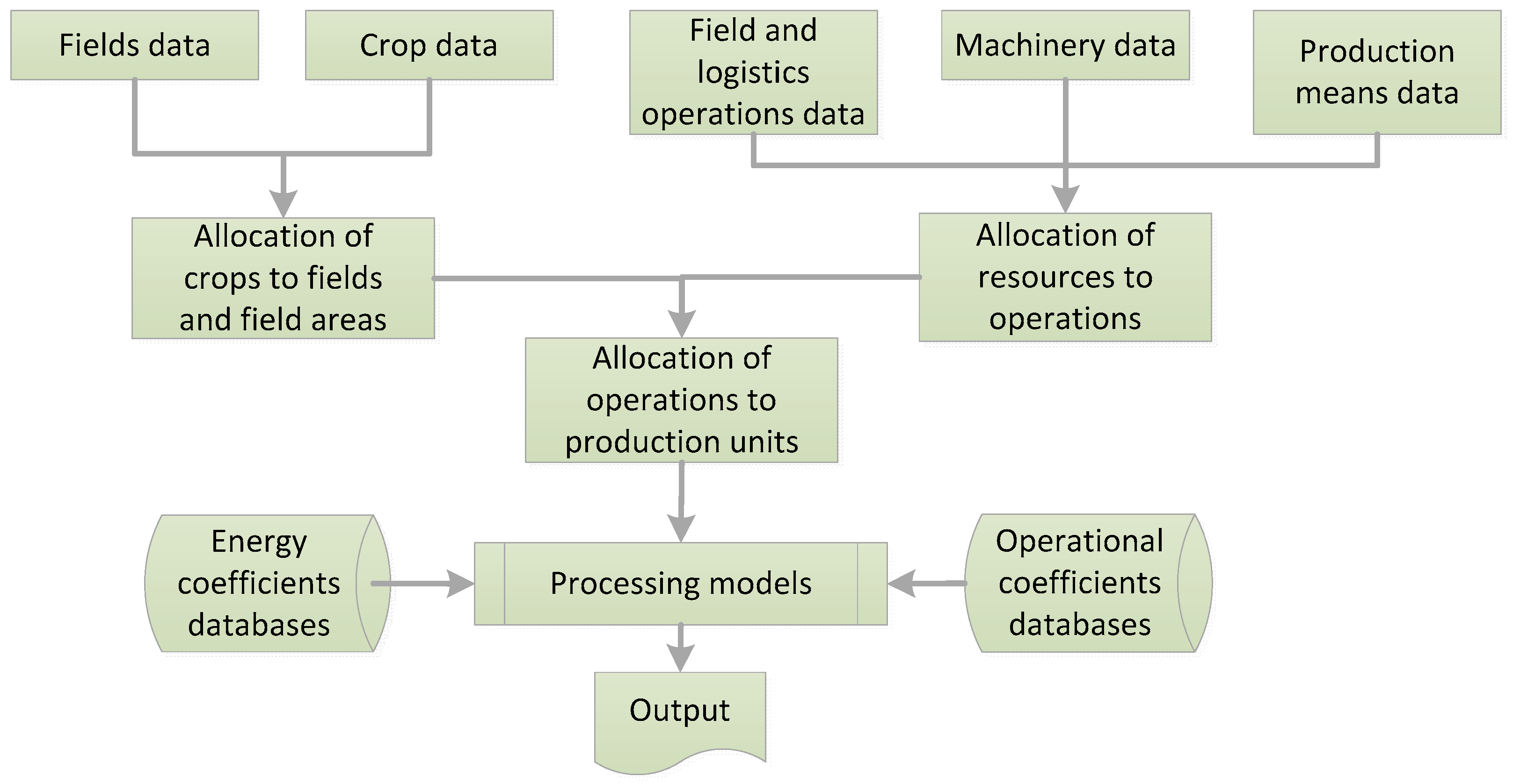
2.1. Overall Description of the System
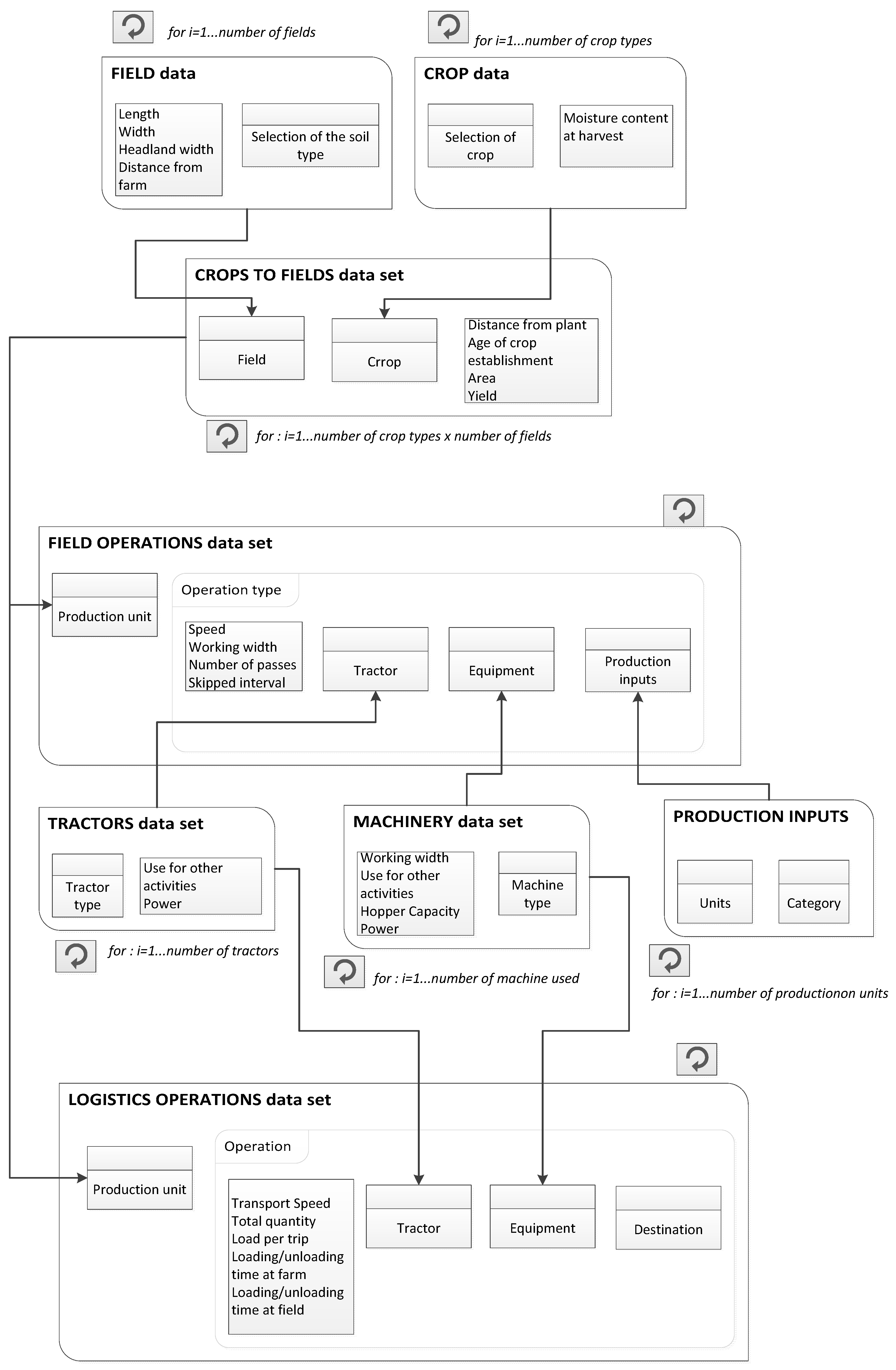
The general structure of the tool is presented in Figure 1. The user provides a series of input data regarding the fields, crops, machines, in-field and logistics operations, and productions means. Based on these data, various entities such as crop groups, field groups, and production units (a field or a field area with a specific crop) are generated by the tool. Then, a series of processing models are applied using also several embedded databases, such as the energy coefficients for all means used for the crop production, operational coefficients for the estimation of the various task times and power requirements for all machinery involved in field and logistics operations.
Figure 1.
The overall structure of the tool.
The object-oriented language ASP.NET MVC is used for building the tool, combined with an SQL Server database used for the generation of the energy requirements estimation models.
2.2. Input
In the material to follow, the main inputs provided by the user are discussed. The input that is provided by the user remains the same as in the case of the cost estimation [20]. To that effect, only the new features of the tool are detailed in this work, while the existing ones are briefly presented. To that end, it is recommended that the reader refer to the above-mentioned paper [20].
2.2.1. Fields and Crops Data
For each individual field, the user provides a series of input parameters related to the geometrical features of the field (Figure 2) and its workability (i.e., soil texture). The soil texture classification (i.e., fine, medium, and coarse) is required for the selection (from the embedded database) of the parameters used for the estimation of the machinery power requirements (necessary for computing the fuel consumption of a specific operation in a particular field) [21]. As regards the cultivated crops, the user selects them iteratively from a list provided by the tool (Figure 2). In the next step, the allocation of crops to each individual field is realized. For each field, the distance from the facility that the crop has to be transported after harvesting is provided by the user, since the facility could be different in type (or in a different location) for different crops and also from the same crop for different fields depending on their location. Finally, the age of the crop establishment for perennial crops (e.g., poplar, willow, and giant reed) has to be defined, since the operations to be performed heavily depend on the age of the crop.
Figure 2.
The input provided by the user to the tool.
2.2.2. Resources
Resources refer to the machinery (e.g., tractors, equipment, and self-propelled machines) and the productive means (e.g., agrochemicals and propagation means). Regarding the machinery input, the annual use of the machine in other activities is an input parameter, since for the estimation of the indirect energy cost of a particular machine the total annual use (both the use within the production system under question and also the use outside its boundaries) has to be taken into account. All the inserted inputs are connected with an embedded database that provides all the operation-specific coefficients related to the operational performance of the particular machinery. For example, set-up times, turning times, etc. and also machinery-specific parameters, such as the repair and maintenance coefficients and the average lifetime, are required for the estimation of the direct and indirect energy requirements.
Regarding the production means, a list is provided by the tool to be selected by the user. The tool has the capability to provide the appropriate coefficients for each one of the production means selected by the user.
2.3. Embedded Databases
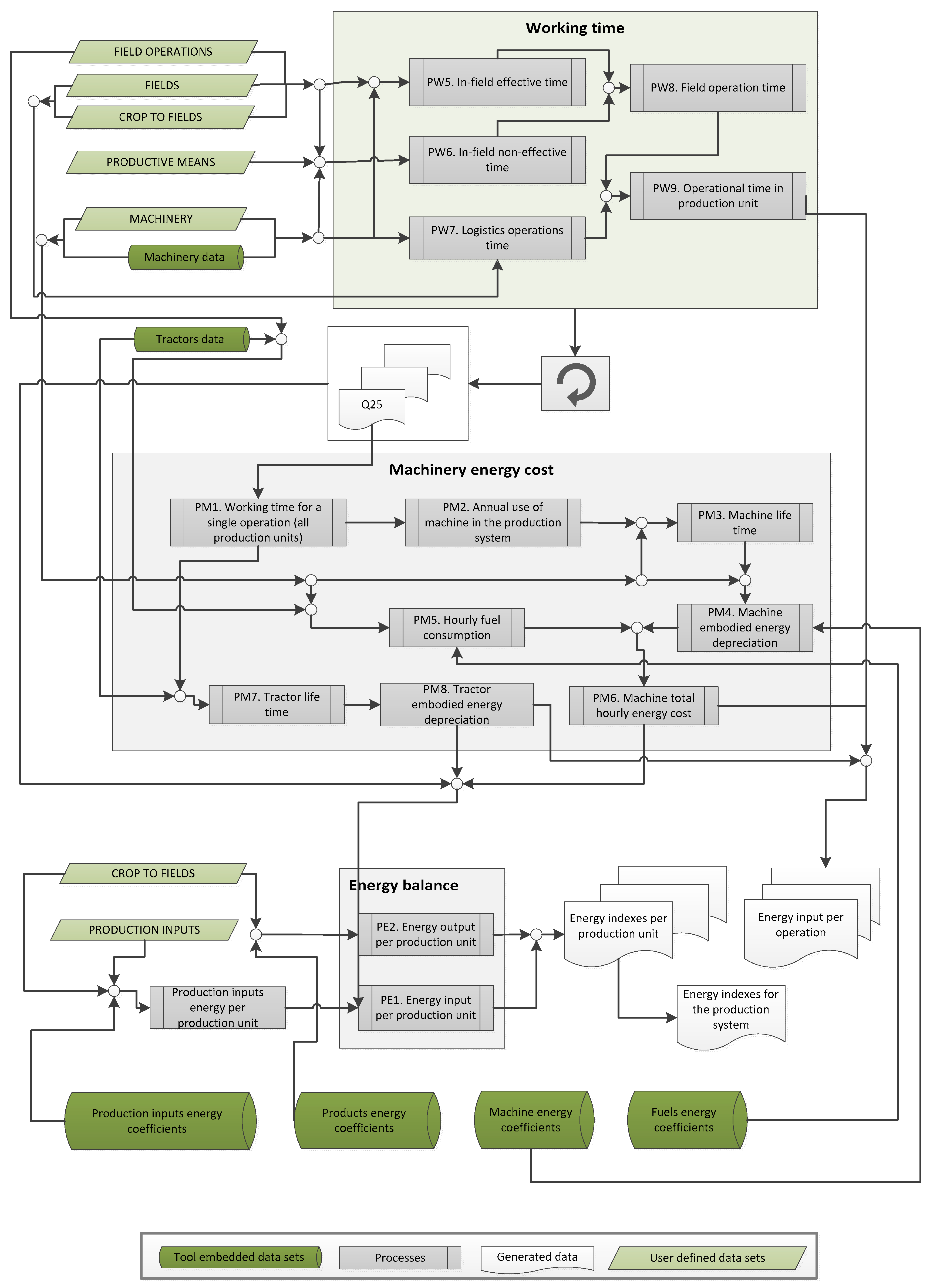
The tool provides to the user a number of lists to select the inputs necessary to design the operational system (type of operations, implemented machinery, etc.) for each production unit (Figure 2). The embedded databases include information for a total of 78 crops. Specifically, information includes data on the yield range, the moisture content range, and the energy content of the dry matter. The embedded databases of the tool involve two types of coefficients: the operations-related and the energy-related ones. The operations-related coefficients [18,20] are necessary in order to calculate the time requirements for each individual operation, including all time elements (e.g., turning time, preparation time in the field, loading and unloading time, etc.) and the fuel consumption requirements in the various parts of a field operation or a logistics operation. The energy related coefficients refer to the embodied energy per unit mass of the various resources implemented or used in the production system. All energy coefficients that are embedded in the tool have been taken from the related literature (Table 1).
Table 1.
Indicative resources for the embedded databases on the energy coefficients.
2.4. Process
As a first step, the operating time for each field operation and logistics operation is calculated (Figure 3). The field capacity refers to every specific operation and depends on the tractor, the equipment, and the field characteristics. The working time includes two parts. Firstly, an effective operating time, which is the time that the machine actually produce work, and, secondly, a non-effective operating time part, which includes any auxiliary time required for performing the operation, such as turning time, unloading time, and tuning time of the machine in the field. For every individual field, the calculation of the in-field working travelled distance is performed. The latter takes into account the number and the length of the field-work tracks, as those generated by the tool. Then, for each individual operation on the specific field, based on the operating speed that is provided by the user, the effective operating time is estimated. For the estimation of the non-effective time during headland turnings, the number of turns is calculated based on the operating width of the equipment and the field dimensions. The times for the various machine adjustments and the other auxiliary times, such as the ones corresponding to loading and unloading activities in operations involving material handling, are provided from the databases of the tool.
Figure 3.
The process for the estimation of the energy requirements of the system.
The fuel consumption (Figure 3) is estimated based on the equation for measuring specific volumetric fuel consumptions given by the ASAE Standards [21]. The data provided by the tool include:
- The required tractive efficiency for a specific operation. Tractive efficiency is used for the estimation of the equivalent PTO (power-take-off).
- The rotary power requirement parameters, also required for the estimation of the equivalent PTO.
- The soil texture adjustment parameter, required for the estimation of the implement draft according to the soil category that has been specified by the user for a specific field.
- The machine parameters, required for the estimation of the implement draft.
Once field capacity has been estimated, the machinery (tractor or equipment) energy depreciation (Figure 3) is calculated by [31]:
where is the embodied energy per unit mass of the machinery (MJ kg−1), M is the mass of the machinery (kg), is the useful lifetime of the machinery (h), and is the field capacity of the specific operation (ha h−1). In the case that a machine is committed to a number of operations, n, then the annual use of the machine is given by:
where is the time spent by the machine in operation i, and is the time spent by the machine in other uses outside the boundaries of the particular production system.
Assuming that a machine is not used more than 20 year, the economic life of the machine is given by:
where, is the economic life (year) and is the lifetime of the machine (h). The lifetime of the machine is provided by an embedded database of the tool built upon ASAE standards [21]. Then, the useful life of the machine can be written as:
In the case of the cost estimation, various external services are taken as a direct input number (e.g., for example the cost of irrigation or the cost of hiring a machine). However, in the case of the energy cost estimation, any external service that adds to the energy input of the production needs to be considered. To this end, a model for the estimation of the irrigation energy requirements is also developed. The model considers the energy consumption for irrigation at the required water flow and pressure. All friction losses in pipes for pressure irrigation (e.g., giant rain gun self-moving equipment, micro-sprinkler irrigation, and the drip irrigation system) are assumed based on relevant literature [43].
2.5. Output
For the production system, the following indices are generated by the tool:
EI: Energy input (MJ), represents the energy required to produce the product in any given field or a given production system.
EO: Energy output (MJ), represents the embodied energy of the product in any given field or in a given production system.
EIUA: Energy input per unit area (MJ ha−1).
EOUA: Energy output per unit area (MJ ha−1).
EIUM: Energy input per unit mass (MJ t−1), which express the energy intensity as defined in Veiga et al. [31].
EB: Energy balance (MJ), expresses the difference: EB = EO − EI.
EBUA: Energy balance per unit area (MJ ha−1), expresses the difference: EBUA = EOUA − EIUA.
EROI: Energy return to investment (dimensionless) as the ratio: EROI = EOUA/EIUA. This index express how much energy output could be produced by one unit of input energy.
The EBUA and EROI indices are considered as most appropriate for energy crops, since they incorporate both the input and output of the process. Accordingly, for food and byproducts, the EI (or EIUA and EIUM) are more suitable and can serve as the functional unit of any given crop [31].
2.6. Case Study Description
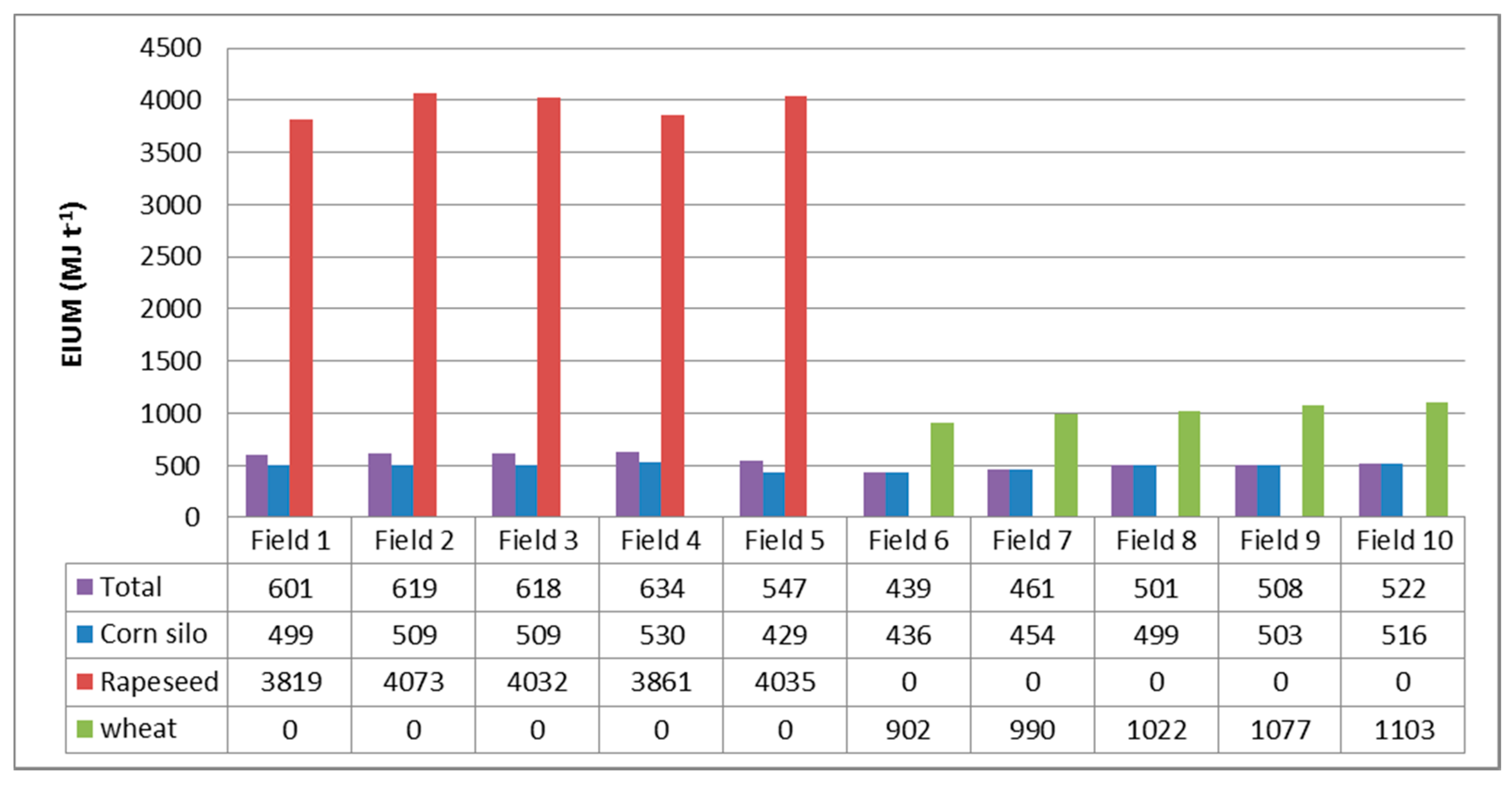
A case study involving a crop production system of 80 ha that feeds a biogas plant of 200 kW is selected for the demonstration of the tool’s applicability. The same production scenario is also presented in Busato and Berruto [20]. The case study is selected to be identical for comparability reasons of the monetary cost and the energy cost contribution of the various operations. The production system refers to three different crops: corn silo, wheat, and rapeseed. Corn silo is cultivated during summer, while the other two are winter crops, cultivated during the rest of the year. The crops are allocated to ten geographically dispersed fields with various areas. Two different irrigation systems are considered for the irrigation of corn silo: the mobile rain gun system (MRS) and the system of drip microirrigation (MCI). The use of different irrigation systems implies different energy inputs for providing the same depth of water quantity per field area unit.
The features of the production system are presented in Table 2. The various field operations and logistics operations for each crop are listed in Table 3 and Table 4, respectively, while the machinery features are provided in Table 5. The machinery for the harvesting operations, namely the combine harvester, the forage harvester, and the baler, are assumed (as in the real system) to be hired. It is worth noting that for the estimation of the monetary cost of these operations, only the cost of hiring the corresponding machinery is taken into account as a pre-fixed input. In the contrary, in the case of the energy cost estimation, these operations have to be analyzed in the same manner as all other operations independently whether it regards own or hired machinery.
Table 2.
Fields and crops characteristics.
Table 3.
Field operations for the various crops.
Table 4.
Logistics operations for the various crops.
Table 5.
Machinery features.
The average yield for the various crops is estimated as follows: corn silo: 50,000 kg ha−1; rapeseed: 3900 kg ha−1; wheat grain: 4350 kg ha−1; and wheat straw: 4800 kg ha−1.
3. Results
Figure 4 presents the contribution in terms of the energy input requirements of each operation, both field operations and logistics operations, for each one of the crops within the production system. This contribution refers to the energy input from the machinery use and not the embedded energy of the production inputs (e.g., fertilizer) in the case of operations where such an input is involved. The field operations that present the highest contribution (FO1 and FO21) are the ones related to organic fertilizer distribution. For these operations, the energy requirements are calculated as approximately 2000 MJ ha−1. The high value of the energy requirements mainly results from the high amount of material that has to be transported and applied in the field in the case of organic fertilizing. For the examined case, the latter amounts 56 t ha−1 (for both silo corn and wheat crops). Based on the results, for the case of corn, the organic fertilizer application, working time per unit area and for the specific selected machinery system, is on average 5.82 h ha−1 (for the case of wheat 4.09 h ha−1), ranging from 3.55 h ha−1 (for the case of wheat 3.34 h ha−1) for field F1, which is located 0.8 km from the farm facilities, up to 9.4 h ha−1 (for the case of wheat 5.21 h ha−1) for field F10, which is located at the furthest distance of 14 km from the farm facilities.
Figure 4.
The contribution of the field and logistics operations for each one of the produced crops.
Plowing operations have similar contribution among crops, with a slight increase for the case of rapeseed because of the longer distance between the farm facilities and the fields where rapeseed is allocated.
The energy requirements in logistics operations are influenced by the transport distance, the implemented machinery system, and the amount of the product to be transported from the field to the facilities. The amount of the product is a function of the crop type and the yield. This is the main reason why logistics operation in corn silo (LO1) requires the highest energy among the crops of the production system (2.964 MJ ha−1). For the case of the wheat, there are two logistics operations, one for the grain (LO3) and one for the straw (LO4) transportation. The energy requirements for both operations are low because fields are located nearby the facilities and the yield of wheat is below 5 t ha−1 for both products.
The energy requirements for the production inputs are presented in Table 6. It becomes obvious that fertilizers have a high contribution in the energy input. In contrast, organic fertilizer, (digestate) as a by-product of the biogas system, is considered as a “zero energy” input. In this case, savings in energy input are considerable, and provide better EROI and EB indices (as presented in Table 7).
Table 6.
Energy requirements for the input resources.
Table 7.
Energetic indexes for single crop and for the entire production system.
Table 7 presents the energetic indices for each crop type for the whole production system. It is evident that crops with higher biomass output (yield) present improved energy balance per unitary area (EBUA). Corn silo exploits better the use of the land with very good positive energy balance per unitary area. Rapeseed provides the lowest yield (120 GJ ha−1). The winter crops (wheat and rapeseed) do not require irrigation. Wheat provides a better EROI, equal on average to 15.21, also because two products are being harvested from the same crop (grain and straw).
It should also be highlighted that EBUA of the whole system is higher than the one for a single crop. This is mainly due to the fact that crop rotation takes place in each single field exploiting half of the area (40 ha) twice a year (either corn followed by rapeseed or corn followed by wheat).
The EROI index is presented on detail in Figure 5 for each individual production unit (field and crop). As mentioned earlier, the crop with the higher performance in terms of EROI is the wheat due to the exploitation of the two types of biomass that produces and due to the fact that wheat is not irrigated. The stepping decrease of the EROI index for the wheat from field F6 to F10 shows the effect on the EROI of the increasing distance between the field and the facilities. In Figure 5, the slightly better performance in terms of EROI of the corn silo compared to the rapeseed can also be detected.
Figure 5.
The energy return on investment (EROI) index for each individual crop and individual field.
Figure 6 presents the EIUM index for each of the crops in the production system in all individual fields. Rapeseed provides the highest EIUM compared to the other crops and this is mainly because the final biomass product that provides energy is oil seeds with a low yield compared to the other crops. However, the output is comparable to the other crops (Figure 5) due to the high energy content of the seeds. The small differences in EIUM between the various fields for the same crop is a result of the different practices followed, the field area, and the distance that biomass is transported.
Figure 6.
The energy input per unit mass (EIUM) (MJ t−1) index for each individual crop and each individual field.
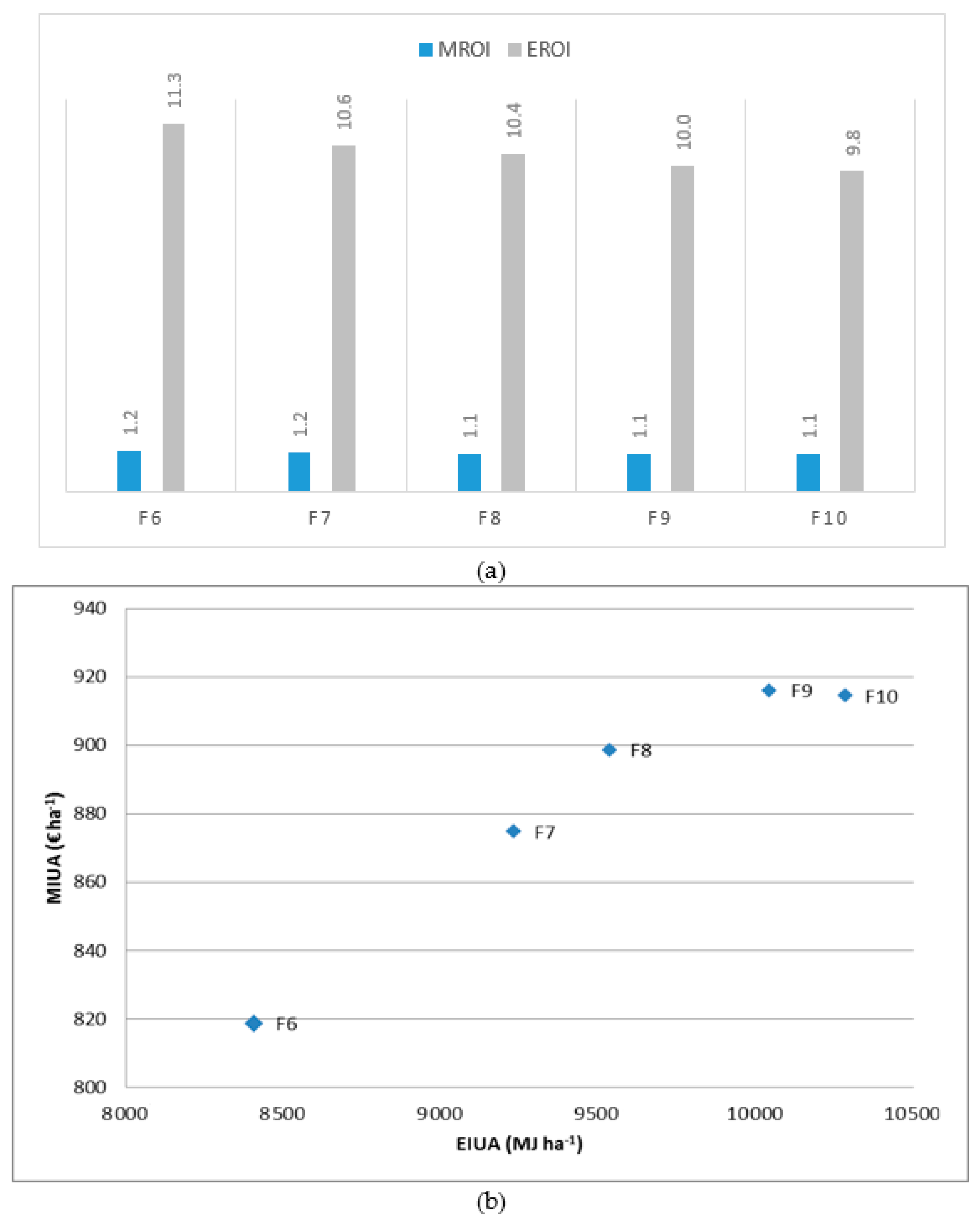
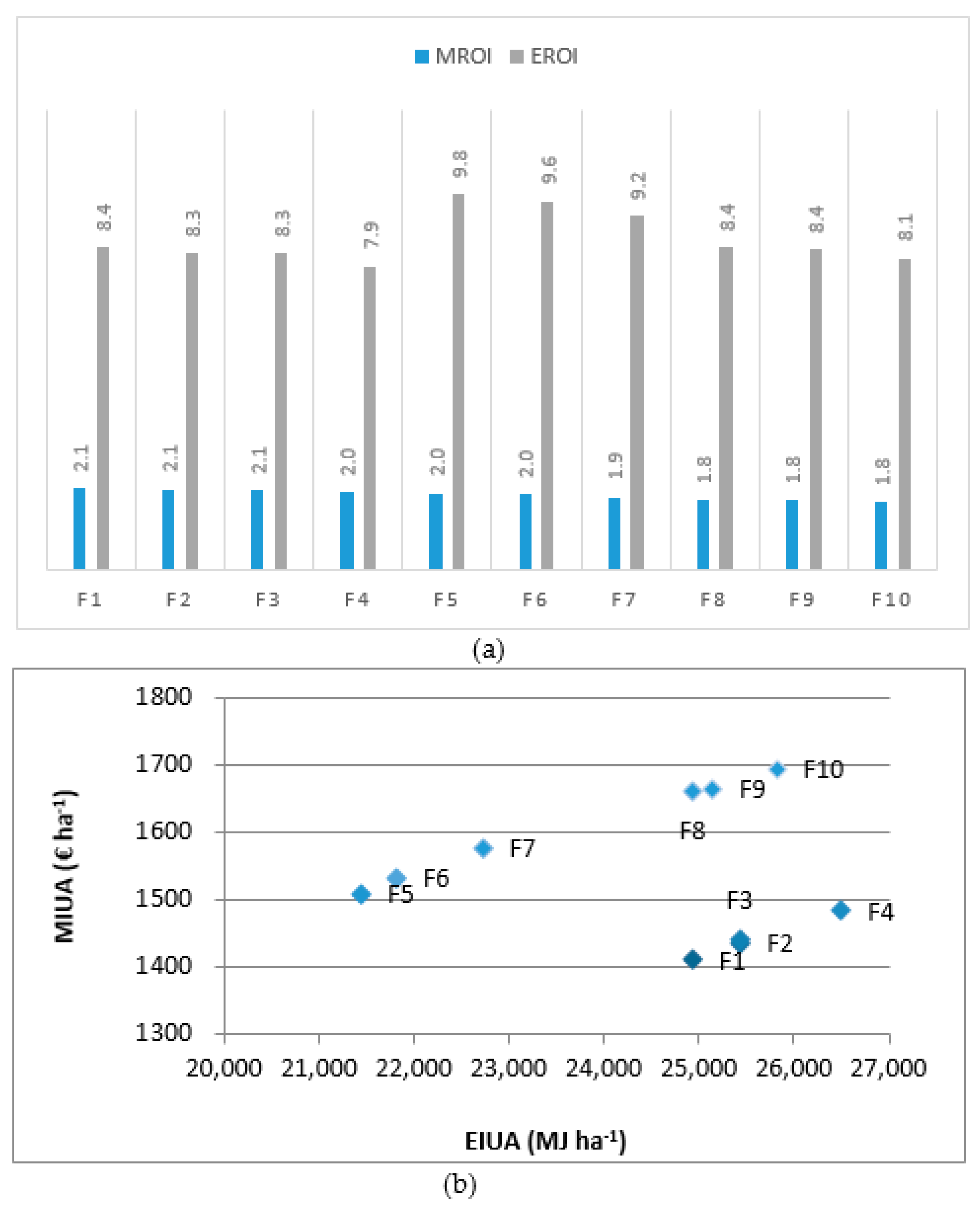
4. Relation between the Energy and Economic Indexes of the Production
In this section, the production system is evaluated in terms of the relation between the energy indexes and the economic ones. For this purpose, the output of the energy assessment of the system provided here is linked with the economic assessment of the system, as provided in Busato and Berruto [20], since both works refer to the same production system and to identical operations input parameters. In order to investigate the relation between energetic and economic performance of each one of the cultivated crops, the EROI is compared with the corresponding index of the economic performance, namely the MROI (monetary return on investment) [20], and the EIUA is compared to the MIUA (monetary input per unit area, € ha−1) [20].
Figure 7a presents the values of the EROI and MROI indexes for the case of the corn silo crop for each individual field. The coefficient of variation for the various fields is 7.62% for the EROI (mean: 8.64, STD: 0.66) while for MROI is 6.65% (mean: 1.95, STD: 0.13). The variations of the two indexes are very close. However, for the case of EROI, the different irrigation systems result to a high variation of the energy requirements, since MRS system consumes on average 11,500 MJ ha−1 while the MCI system consumes on average 5500 MJ ha−1. This explains the difference in the energy requirements, for example, between F4 (EROI: 7.9) and F5 (EROI: 9.8), where energy requirements are 26,500 MJ ha−1 and 21,446 MJ ha−1, respectively. On the other hand, the irrigation system applied does not affect the cost and thus the MIUA is almost the same for the two fields (Figure 7b). In terms of the EIUA and MIUA relation, the linear relation for fields F5–F10 and the one for fields F1–F4 is explained by the different irrigation system applied to the two sets of fields.
Figure 7.
The EROI and monetary return on investment (MROI) indexes (a); and the Energy input per unit area (EIUA) and monetary input per unit area (MIUA) (b) for each corn silo fields (F stands for “field”).
For the case of rapeseed production (Figure 8a), the coefficient of variation for the various fields is 2.93% for the EROI (mean: 7.83, STD: 0.23) while for MROI is 3.71% (mean: 1.71, STD: 0.06). The relatively small and comparable variation in the EROI and MROI indexes, which is also explained by the linear relation between the EIUA and MIUA indexes (Figure 8b), is a result of the identical operations applied to all fields and the small distances of all fields where rapeseed is cultivated from the storage facilities.
Figure 8.
The EROI and MROI indexes (a); and the EIUA and MIUA (b) for each rapeseed fields (F stands for “field”).
For the case of wheat production (Figure 9a), the coefficient of variation for the various fields is 8.07% for the EROI (mean: 14.84, STD: 1.20) while for MROI is 4.75% (mean: 0.96, STD: 0.05). The higher variation in both economic and energy indexes in the case of wheat compared to the variation in indexes of the other crops has to do with the higher variation of the distances between the fields where wheat is cultivated and the storage facilities.
Figure 9.
The EROI and MROI indexes (a); and the EIUA and MIUA (b) for each wheat fields (F stands for “field”).
5. Conclusions
A web-based tool for the energy balance assessment of crop production systems feeding bioenergy plants that involves multiple crops cultivated in multiple fields is presented in this work. The energy input accounting refers to the whole supply chain of the biomass, including the crop cultivation (soil preparation, seeding, planting, fertilizing, spraying, etc.), harvesting, handling of the biomass, and biomass transportation to the processing or storage facilities. The tool takes into consideration the individual features of each production unit (i.e., a specific field with a specific crop), such as the specific machinery system, soil conditions, travelling distances, and various operational and agronomic parameters. The inclusion of these parameters provides an accurate estimation of the energy requirements for a specific system diversifying the presented tool from other existing tools that are based on average values. However, the accurate values of all parameters are a prerequisite for the production of qualified results by the tool. Furthermore, another limitation of the tool is the absence of embedded models that could correlate the yield with the various inputs, e.g., irrigation and fertilizers, as well as the effect of the weather conditions in an area on the yield performance. The above-mentioned issues are considered by the authors as future research challenges.
The tool can be used for the comparison of the performance in terms of energy requirements and balance between various crops, fields, operational practices and systems providing support for decisions on the biomass production system design (e.g., allocation of crops to fields) and operations management (e.g., machinery system selection). Moreover, the presented tool is a continuation of the corresponding web-tool for the cost evaluation of multiple-crops production systems that has been previously developed; and can be used for the consideration of the performance of a system in terms of energy cost against its performance in terms of monetary cost, since various practices and operational options (e.g., irrigation system, contracting machinery, etc.) have diversified effect on the energetic and economic performance of the system.
Due to its high flexibility for simulating numerous configurations of a production system, the presented web tool can be used to assess almost any farm performance in terms of energy balance and thus verify a specific biofuel cultivation system toward the renewable energy directive (RED 2009) emission limits.
Acknowledgments
This work was part of the collaborative research project Bio-Energy Farm II. The research leading to these results has received funding from the Intelligent Energy Europe Programme under grant agreement no. IEE/12/683/SI2.675767.
Author Contributions
Patrizia Busato, Alessandro Sopegno, Remigio Berruto, Dionysis Bochtis, Angela Calvo contributed equally to the single step of the work. All authors read and approved the final manuscript.
Conflicts of Interest
The authors declare no conflict of interest.
Abbreviations
The following abbreviations are used in this manuscript:
| EB | Energy balance per unit area |
| EI | Energy input |
| EIUA | Energy input per unit area |
| EIUM | Energy input per unit mass |
| EO | Energy output |
| EOU | Energy output per unit area |
| EROI | Energy return to investment |
| MCI | Microirrigation system |
| MIUA | Monetary input per unit area |
| MROI | Monetary return on investment |
| MRS | Mobile rain gun irrigation system |
| PTO | Power take off |
References
- De Besi, M.; McCormick, K. Towards a bioeconomy in Europe: National, regional and industrial strategies. Sustainability 2015, 7, 10461–10478. [Google Scholar] [CrossRef]
- Ba, B.H.; Prins, C.; Prodhon, C. Models for optimization and performance evaluation of biomass supply chains: An Operations Research perspective. Renew. Energy 2016, 87, 977–989. [Google Scholar] [CrossRef]
- Pinho, T.M.; Coelho, J.P.; Moreira, A.P.; Boaventura-Cunha, J. Modelling a biomass supply chain through discrete-event simulation. IFAC Pap. OnLine 2016, 49, 84–89. [Google Scholar] [CrossRef]
- Zhang, F.; Johnson, D.M.; Johnson, M.A. Development of a simulation model of biomass supply chain for biofuel production. Renew. Energy 2012, 44, 380–391. [Google Scholar] [CrossRef]
- Pavlou, D.; Orfanou, A.; Busato, P.; Berruto, R.; Sørensen, C.; Bochtis, D. Functional modeling for green biomass supply chains. Comput. Electron. Agric. 2016, 122, 29–40. [Google Scholar] [CrossRef]
- Gissén, C.; Prade, T.; Kreuger, E.; Nges, I.A.; Rosenqvist, H.; Svensson, S.-E.; Lantz, M.; Mattsson, J.E.; Börjesson, P.; Björnsson, L. Comparing energy crops for biogas production—Yields, energy input and costs in cultivation using digestate and mineral fertilisation. Biomass Bioenergy 2014, 64, 199–210. [Google Scholar] [CrossRef]
- Börjesson, P.; Tufvesson, L.M. Agricultural crop-based biofuels—Resource efficiency and environmental performance including direct land use changes. J. Clean. Prod. 2011, 19, 108–120. [Google Scholar] [CrossRef]
- Kavargiris, S.E.; Mamolos, A.P.; Tsatsarelis, C.A.; Nikolaidou, A.E.; Kalburtji, K.L. Energy resources’ utilization in organic and conventional vineyards: Energy flow, greenhouse gas emissions and biofuel production. Biomass Bioenergy 2009, 33, 1239–1250. [Google Scholar] [CrossRef]
- Michos, M.C.; Mamolos, A.P.; Menexes, G.C.; Tsatsarelis, C.A.; Tsirakoglou, V.M.; Kalburtji, K.L. Energy inputs, outputs and greenhouse gas emissions in organic, integrated and conventional peach orchards. Ecol. Indic. 2012, 13, 22–28. [Google Scholar] [CrossRef]
- Liu, Y.; Langer, V.; Høgh-Jensen, H.; Egelyng, H. Energy Use in Organic, Green and Conventional Pear Producing Systems—Cases from China. J. Sustain. Agric. 2010, 34, 630–646. [Google Scholar] [CrossRef]
- Strapatsa, A.V.; Nanos, G.D.; Tsatsarelis, C.A. Energy flow for integrated apple production in Greece. Agric. Ecosyst. Environ. 2006, 116, 176–180. [Google Scholar] [CrossRef]
- Milà i Canals, L.; Burnip, G.M.; Cowell, S.J. Evaluation of the environmental impacts of apple production using Life Cycle Assessment (LCA): Case study in New Zealand. Agric. Ecosyst. Environ. 2006, 114, 226–238. [Google Scholar] [CrossRef]
- Kaltsas, A.M.; Mamolos, A.P.; Tsatsarelis, C.A.; Nanos, G.D.; Kalburtji, K.L. Energy budget in organic and conventional olive groves. Agric. Ecosyst. Environ. 2007, 122, 243–251. [Google Scholar] [CrossRef]
- Zafiriou, P.; Mamolos, A.P.; Menexes, G.C.; Siomos, A.S.; Tsatsarelis, C.A.; Kalburtji, K.L. Analysis of energy flow and greenhouse gas emissions in organic, integrated and conventional cultivation of white asparagus by PCA and HCA: Cases in Greece. J. Clean. Prod. 2012, 29, 20–27. [Google Scholar] [CrossRef]
- Litskas, V.D.; Mamolos, A.P.; Kalburtji, K.L.; Tsatsarelis, C.A.; Kiose-Kampasakali, E. Energy flow and greenhouse gas emissions in organic and conventional sweet cherry orchards located in or close to Natura 2000 sites. Biomass Bioenergy 2011, 35, 1302–1310. [Google Scholar] [CrossRef]
- Stolarski, M.J.; Krzyżaniak, M.; Tworkowski, J.; Szczukowski, S.; Gołaszewski, J. Energy intensity and energy ratio in producing willow chips as feedstock for an integrated biorefinery. Biosyst. Eng. 2014, 123, 19–28. [Google Scholar] [CrossRef]
- Sørensen, C.G.; Halberg, N.; Oudshoorn, F.W.; Petersen, B.M.; Dalgaard, R. Energy inputs and GHG emissions of tillage systems. Biosyst. Eng. 2014, 120, 2–14. [Google Scholar] [CrossRef]
- Sopegno, A.; Rodias, E.; Bochtis, D.; Busato, P.; Berruto, R.; Boero, V.; Sørensen, C. Model for energy analysis of Miscanthus production and transportation. Energies 2016, 9, 392. [Google Scholar] [CrossRef]
- Busato, P.; Sørensen, C.G.; Pavlou, D.; Bochtis, D.D.; Berruto, R.; Orfanou, A. DSS tool for the implementation and operation of an umbilical system applying organic fertiliser. Biosyst. Eng. 2013, 114, 9–20. [Google Scholar] [CrossRef]
- Busato, P.; Berruto, R. A web-based tool for biomass production systems. Biosyst. Eng. 2014, 120, 102–116. [Google Scholar] [CrossRef]
- ASAE D497.5. Agricultural machinery management data. In ASABE STANDARD 2009, Vol. I; American Society of Agricultural and Biological Engineers: St. Joseph, MI, USA, 2009; pp. 360–367. [Google Scholar]
- Pimentel, D. Handbook of Energy Utilization in Agriculture; CRC Press, Inc.: Boca Raton, FL, USA, 1980. [Google Scholar]
- Nagy, C. Energy Coefficient for Agriculture Inputs in Western Canada; University of Saskatchewan: Saskatoon, SK, Canada, 1999. [Google Scholar]
- Chamsing, A.; Salokhe, V.M.; Singh, G. Energy Consumption Analysis for Selected Crops in Different Regions of Thailand. Agric. Eng. Int. 2006, VIII, 1–18. [Google Scholar]
- Nassiri, S.M.; Singh, S. Study on energy use efficiency for paddy crop using data envelopment analysis (DEA) technique. Appl. Energy 2009, 86, 1320–1325. [Google Scholar] [CrossRef]
- Dalgaard, T.; Halberg, N.; Porter, J.R. A model for fossil energy use in Danish agriculture used to compare organic and conventional farming. Agric. Ecosyst. Environ. 2001, 87, 51–65. [Google Scholar] [CrossRef]
- ASAE EP496.3. Agricultural machinery management. In ASABE STANDARD 2009; ASABE, Ed.; American Society of Agricultural and Biological Engineers: St. Joseph, MI, USA, 2009; Volume I, pp. 354–357. [Google Scholar]
- Hülsbergen, K.-J.; Feil, B.; Biermann, S.; Rathke, G.-W.; Kalk, W.-D.; Diepenbrock, W. A method of energy balancing in crop production and its application in a long-term fertilizer trial. Agric. Ecosyst. Environ. 2001, 86, 303–321. [Google Scholar] [CrossRef]
- Ozturk, H.H.; Ekinci, K.; Barut, Z.B. Energy analysis of the tillage systems in second crop corn production. J. Sustain. Agric. 2006, 28, 25–37. [Google Scholar] [CrossRef]
- Rathke, G.W.; Diepenbrock, W. Energy balance of winter oilseed rape (Brassica napus L.) cropping as related to nitrogen supply and preceding crop. Eur. J. Agron. 2006, 24, 35–44. [Google Scholar] [CrossRef]
- Veiga, J.P.S.; Romanelli, T.L.; Gimenez, L.M.; Busato, P.; Milan, M. Energy embodiment in Brazilian agriculture: An overview of 23 crops. Sci. Agric. 2015, 72, 471–477. [Google Scholar] [CrossRef]
- Romanelli, T.L.; Milan, M. Material flow determination through agricultural machinery management. Sci. Agric. 2010, 67, 375–383. [Google Scholar] [CrossRef]
- Gubiani, R.D. Corn utilization in a family-boiler: Greenhouse emissions, economic estimation and energy assessment. In Agricultural and Biosystems Engineering for a Sustainable World; European Society of Agricultural Engineers: Hersonissos, Greece, 2008. [Google Scholar]
- Persson, T.; Paz, J.; Hoogenboom, G.; Garcia, A.G.Y.; Jones, J.W. Net energy value of maize ethanol as a response to different climate and soil conditions in the southeastern USA. Biomass Bioenergy 2009, 33, 1055–1064. [Google Scholar] [CrossRef]
- Piringer, G.; Steinberg, L.J. Reevaluation of energy use in wheat production in the United States. J. Ind. Ecol. 2006, 10, 149–167. [Google Scholar] [CrossRef]
- Ray, S.; Pramanick, M.; Mani, P.K.; Roy, K.; Sengupta, K.M.C.; Ray, S.; Pramanick, P.K.; Roy, K.M.; Chatterjee, M.; Mani, K.S. Diversification of rice-based cropping system and their impact on energy utilization and system production. J. Crop Weed 2009, 5, 167–170. [Google Scholar]
- Deike, S.; Pallutt, B.; Christen, O. Investigations on the energy efficiency of organic and integrated farming with specific emphasis on pesticide use intensity. Eur. J. Agron. 2008, 28, 461–470. [Google Scholar] [CrossRef]
- Swanton, C.J.; Murphy, S.D.; Hume, D.J.; Clements, D.R. Recent improvements in the energy efficiency of agriculture: Case studies from Ontario, Canada. Agric. Syst. 1996, 52, 399–418. [Google Scholar] [CrossRef]
- Pimentel, D.; Pimentel, M.; Karpenstein, M. Energy use in agriculture: An overview. CIGR E J. 1999, 1, 1–32. [Google Scholar]
- Venturi, P.; Venturi, G. Analysis of energy comparison for crops in European agricultural systems. Biomass Bioenergy 2003, 25, 235–255. [Google Scholar] [CrossRef]
- Nanda, S.S.; Mohanty, M.; Pradhan, K.C.; Mohanty, A.K.; Mishra, M.M. Production potential, profitability and energy efficient rice based cropping systems for coastal Orissa. J. Farming Syst. Res. Dev. 2008, 14, 1–5. [Google Scholar]
- Hernanz, J.L.; Giron, V.S.; Cerisola, C. Long-term energy use and economic evaluation of three tillage systems for cereal and legume production in central Spain. Soil Tillage Res. 1995, 35, 183–198. [Google Scholar] [CrossRef]
- Boswell, M.J. Hardie Irrigation Micro-Irrigation Design, 4th ed.; Edagricole: Bologna, Italy, 1993. [Google Scholar]
- Pereira, L.S.; Trout, J. Irrigation methods. In CIGR Handbook of Agricultural Engineering, Volume I: Land and Water Engineering; American Society of Agricultural Engineers: St. Joseph, MI, USA, 1999; pp. 297–379. [Google Scholar]
© 2017 by the authors. Licensee MDPI, Basel, Switzerland. This article is an open access article distributed under the terms and conditions of the Creative Commons Attribution (CC BY) license (http://creativecommons.org/licenses/by/4.0/).