An Optimal Dispatch Model of Wind-Integrated Power System Considering Demand Response and Reliability

Abstract

Demand response (DR) has become an impressive option in the deregulated power system due to its features of availability, quickness and applicability. In this paper, a novel economic dispatch model integrated with wind power is proposed, where incentive-based DR and reliability measures are taken into account. Compared with the conventional models, the proposed model considers customers’ power consumption response to the incentive price. The load profile is optimized with DR to depress the influence on the dispatch caused by the anti-peak-shaving and intermittence of wind generation. Furthermore, a probabilistic formulation is established to calculate the expected energy not supplied (EENS). This approach combines the probability distribution of the forecast errors of load and wind power, as well as the outage replacement rates of units into consideration. The cost of EENS is added into the objective to achieve an optimal equilibrium point between economy and reliability of power system operation. The proposed model is solved by mixed integer linear programming (MILP). The applicability and effectiveness of this model is illustrated by numerical simulations tested on the IEEE 24-bus Reliability Test System.

1. Introduction

To deal with a growing threat from the energy crisis and the climatic variation, there has been a great increase in the utilization of wind power as an alternative to fossil fuels. While wind power retains many advantages such as lower operating cost, less pollutant emission, more flexible capacity and so on, its increasing penetration has brought challenges to electric dispatching [1,2,3,4]. There exist strong randomicity and volatility of wind power, as well as the anti-peak characteristic, which have brought about negative effects on the safe and economic operation of power system [5,6,7,8]. As it is difficult to predict wind power with great accuracy, how to evaluate the impact of forecast errors on reliability is of fundamental significance. Furthermore, with the increasing wind capacity integrated into the power grid, it is hardly realistic to coordinate the conventional units for dispatch invariably. Demand response (DR), as an effective means for load scheduling, plays an important role in the electricity market [9,10,11]. Therefore, a novel method on the unit commitment should be developed considering DR and reliability measures due to the errors of prediction on the load and wind power, as well as generation outages.

The reliability assessment is a crucial aspect for consideration in power system integrated with wind power. In the problem of the traditional unit commitment, the spinning reserve is accepted with a certain proportion of the forecast load or the maximum capacity of the operating units. This deterministic means has left out multiple uncertainties, such as the wind forecast error, the load forecast error, and the forced outage rate of units [12,13]. During recent years, the stochastic assessment of the spinning reserve has been applied in many articles [14,15,16]. With this approach, the spinning reserve is optimized to satisfy the expected energy not supplied (EENS). In [17], a triangular approximate distribution model is used to quantify EENS due to the stochastic feature of wind. Then, a security-constrained unit commitment algorithm is proposed to schedule conventional units and wind generation considering probabilistic forecast models of wind power. Another day-head scheduling model involving reliability criteria is described in [18]. EENS is calculated with the historical outage replacement rates of generators or lines. MILP is utilized to deal with the proposed model. In [19], the forecast errors of both wind power and load are supposed to follow normal distributions. These errors are discretized into several intervals for a new formulation of reliability measures. In [20,21], a two-stage stochastic problem is formulated to address various uncertainties in the system, such as wind power, solar generation, loads and even electric vehicles. The sample average approximation, which is a Monte Carlo simulation technique, is utilized to deal with uncertainties for scenario generation purposes. These works have integrated the system with distribution-free uncertainties, but given a rise to the computational burden.

As an effective way for peak load shedding and shaving, DR has been widely investigated in the electricity market. Consuming wind power with DR will result in solving the optimal dispatch problem of wind power integrated system. Nowadays, there have been some researches on the unit commitment with DR. The uncertainties of DR are taken into consideration to deal with the stochastic unit commitment in [22]. In [23], the incentive-based DR and high penetration of wind generation are combined to formulate a probabilistic unit commitment problem. Meanwhile, this model is constrained by n-1 reliability criterion for the optimal allocation of up/down spinning reserve. In [24], demand response programs (DRPs) have been studied on the case that a wind farm is connected to the power grid. The objective function of this model in [24] is to maximize the total social welfare under the constraint of power deficit probability.

Based on existing studies, a novel economic dispatch model considering DR and reliability measures is proposed in this paper. Given the great importance of DR in load scheduling, the incentive-based DR with a dynamic incentive mechanism is combined into the model. To determine the capacity of reserve, a probabilistic approach is developed to calculate EENS. This approach takes into account the probability distribution of the demand and wind power errors, as well as the outage replacement rates of units. Value of lost load (VOLL) is introduced to quantify the cost of EENS. The objective of this model is to obtain a trade-off among the costs of generation, incentives and EENS.

The rest of this paper is organized as follows. Section 2 is dedicated to the evaluation of EENS considering uncertainties. The proposed model of DR is explained in detail in Section 3. Then, the problem formulation is described in Section 4. After that, results of case studies are presented in Section 5. Finally, concluding remarks are drawn in Section 6.

2. Evaluation of EENS Considering Uncertainties

2.1. Uncertainty Model of Load and Wind Power

Usually, the load is forecasted with an error, which is assumed to follow a Gaussian distribution [25,26]. Thus, the actual load can be seen as the sum of the forecast load and the error

$$L_t^A=L_t^F+{\epsilon }_t^L$$

(1)

where $L_{\mathrm{t}}^A$ is the actual load at period $t$, $L_t^F$ is the forecast load at period $t$ and ${\epsilon }_t^L$ is the load forecast error. ${\epsilon }_t^L$ is normally distributed with zero mean and a standard deviation. The standard deviation of the load forecast error ${\delta }_t^L$ can be written as

$${\delta }_t^L=\frac{3}{100}{L}_t^F$$

(2)

Similar to the load, the actual wind power is assumed to consist of the forecast power plus an error. It can be expressed as follows

$$W_t^A=W_t^F+{\epsilon }_t^W$$

(3)

where $W_t^A$ is the actual wind power at period $t$, $W_t^F$ is the forecast wind power at period $t$ and ${\epsilon }_t^L$ is wind power prediction error.

Some papers show that wind power forecast error of a single wind turbine follows a $\beta$ distribution [27,28]. However, the central limit theorem can be applied to the total wind power prediction error of a large number of wind turbines with a rich geographical dispersion. Thus, the total forecast error can be assumed to model as a Gaussian distribution with expectation zero and a standard deviation ${\delta }_{\mathrm{t}}^W$.

$${\delta }_t^W=\frac{1}{5}{W}_t^F+\frac{1}{50}{W}_I$$

(4)

where $W_I$ is the total capacity of the wind farm.

2.2. Formulation of EENS

Traditionally, EENS of power system is aroused by generators out of work. In this paper, both the forecast errors of the load and wind power are taken into consideration. Thus, the EENS is evaluated under the circumstances that the available spinning reserve is less than the forecast errors and the output of unavailable generating units. As we know, the uncertainties of thermal units are a set of binary integer variables, while the forecast errors are continuous ones. To combine the continuous variables with the binary ones, the discretization method is applied to deal with it. In the previous research, the discretization of the net demand forecast error was involved in the expression of EENS, which is defined as the difference between the forecast load and the forecast wind power [19]. This method could not take a full account of the uncertainty of wind power. Thus, on the strength of step-by-step modeling technology, the discretization of the net demand forecast error is extended to that of the forecast load and wind power. Thus, the EENS formulation proposed in this paper is to deal with the forecast error of wind power modeled by different probability distributions. Figure 1 presents a flowchart of the method for calculating EENS in the proposed model.

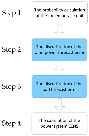
Figure 1. EENS calculation process in the proposed model.

2.2.1. Probability Calculation of the Forced Outage Unit

A binary variable ${\gamma }_{i,t}$ is introduced to indicate the status of unit $i$ at period $t$. Then the probability in case that unit $i$ is scheduled but unavailable is to be expressed as

$${\pi }_{i,t}={\gamma }_{i,t}{U}_i{\displaystyle \prod _{j=1,j\ne i}^{N_{Gen}}(1-{\gamma }_{j,t}{U}_j)}\approx {\gamma }_{i,t}{U}_i$$

(5)

where $U_i$ is the outage replacement rate of unit $i$ and $N_{Gen}$ is the number of all generators.

Under the circumstance that all scheduled units are available or only one unit is shut down, there are a total of $N_{Gen}+1$ initial scenarios that will be constructed. The spinning reserve margin $R{M}_{s,t}$ resulting from the outage of unit $i$ under scenario $s$ is

$$R{M}_{s,t}={\displaystyle \sum _{j=1}^{N_{Gen}}{R}_{j,t}}-(P_{i,t}+R_{i,t})$$

(6)

where $P_{i,t}$ and $R_{i,t}$ are the power supply and spinning reserve capacity of unit $i$ during period $t$, respectively; and $s=0$ indicates that there are no units off-line, $s\in [0,N_{Gen}]$.

2.2.2. Discretization of Wind Power Forecast Error

The standard normal distribution is employed to describe the probability function of the wind forecast error ${\delta }_{\mathrm{t}}^W$. As stated before, the normal distribution is a continuous function, which is unfavorable for calculating and modeling. To discretize it, the probability distribution function of ${\delta }_{\mathrm{t}}^W$ is divided into $K$ intervals with $p_{k_1,t}$ as the probability of interval $k_1$. Then, the mid-value of each interval is taken as the expectation of the whole interval. The larger $K$ is, the more accurate the result is, at the expense of massive calculation. Thus, $K$ is set as 7 in this article, as shown in Figure 2. The weight $p_{k_1,t}$ is given by the area under the normal curve between the lower and upper bounds of interval $k_1$

$$p_{k_1,t}=\frac{1}{{\delta }_{\mathrm{t}}^W\sqrt{2\pi }}{\displaystyle {\int }_{l_{k_1}}^{u_{k_1}}{e}^{-x^2/2{({\delta }_{\mathrm{t}}^W)}^2}}dx$$

(7)

where $l_{k_1}$ and $u_{k_1}$ are lower and upper limits, and $l_{k_1}=(k_1-4-1/2){\delta }_{\mathrm{t}}^W$, $u_{k_1}=(k_1-4+1/2){\delta }_{\mathrm{t}}^W$.

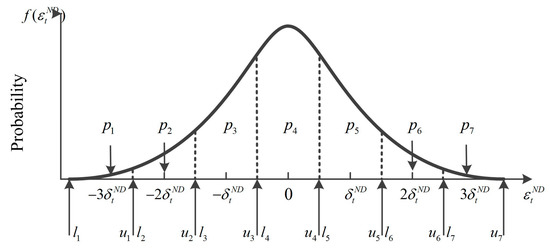
Figure 2. Seven-interval approximation of the normal distribution of the forecast error.

The expectation of interval $k_1$ refers to

$${\epsilon }_{{\mathrm{k}}_1,\mathrm{t}}^W=(k_1-\frac{K+1}{2}){\delta }_{\mathrm{t}}^W$$

(8)

where ${\epsilon }_{{\mathrm{k}}_1,\mathrm{t}}^W$ is the total forecast error of the $k_1$-th interval at period $t$.

If these $K$ intervals of wind power forecast error are incorporated in the $R{M}_{s,t}$ of each initial scenario, $(N_{Gen}+1)K$ new scenarios will be reconstructed. In each new scenario, the spinning reserve margin $R{M}_{s,k_1,t}$ caused by both the wind power forecast error ${\epsilon }_{{\mathrm{k}}_1,\mathrm{t}}^W$ and the outage of unit $i$ is to be expressed as

$$R{M}_{s,k_1,t}=\{\begin{array}{ll}R{M}_{s,t}+{\lambda }_{k_1,t}[(k_1-\frac{K+1}{2}){\delta }_{\mathrm{t}}^W+s_{\mathrm{t}}^W]& k_1\in [1,4]\\ R{M}_{s,t}+(k_1-\frac{K+1}{2}){\delta }_{\mathrm{t}}^W& k_1\in [5,K]\end{array}$$

(9)

where $s_{\mathrm{t}}^W$ is the wind curtailment at period $t$, satisfying $0\le s_{\mathrm{t}}^W\le W_{\mathrm{t}}^F$; ${\lambda }_{k_1,t}$ is a binary variable to decide whether $s_{\mathrm{t}}^W$ has influenced the value of ${\epsilon }_{{\mathrm{k}}_1,\mathrm{t}}^W$ in the interval $k_1$($k_1\le 4$).

${\lambda }_{k_1,t}$ has to fulfill the following condition that

$${\lambda }_{k_1,t}=\{\begin{array}{ll}1& (k_1-\frac{K+1}{2}){\delta }_{\mathrm{t}}^W+s_{\mathrm{t}}^W<0\\ 0& \hspace{1em}\hspace{1em}else\end{array}$$

(10)

In order to solve the proposed model with MILP, the conditional expression of Equation (10) can be equivalent to the linear constraints that

$$-\frac{(k_1-\frac{K+1}{2}){\delta }_{\mathrm{t}}^W+s_{\mathrm{t}}^W}{{\displaystyle \sum _{i=1}^{N_{Gen}}{P}_i^{\max }}}\le {\lambda }_{k_1,t}\le 1-\frac{(k_1-\frac{K+1}{2}){\delta }_{\mathrm{t}}^W+s_{\mathrm{t}}^W}{{\displaystyle \sum _{i=1}^{N_{Gen}}{P}_i^{\max }}}$$

(11)

where $P_i^{\max }$ is the maximum power supply of unit $i$. We can see that the absolute value of $(k_1-\frac{K+1}{2}){\delta }_{\mathrm{t}}^W+s_{\mathrm{t}}^W$ is smaller than ${\displaystyle \sum _{i=1}^{N_{Gen}}{P}_i^{\max }}$. From Equation (11), if $(k_1-\frac{K+1}{2}){\delta }_{\mathrm{t}}^W+s_{\mathrm{t}}^W<0$, the lower bound of Equation (11) should be strictly in the interval of (0,1), while the upper bounds is greater than 1 and less than 2. Thus, ${\lambda }_{k_1,t}$ is equal to 1 if the wind curtailment $s_{\mathrm{t}}^W$ has an impact on ${\epsilon }_{{\mathrm{k}}_1,\mathrm{t}}^W$. Otherwise, ${\lambda }_{k_1,t}$ will take the value 0.

2.2.3. Discretization of the Load Forecast Error

Similar to the wind power forecast error, the standard normal distribution of the load forecast error can be discretized onto $K$($K=7$) intervals as well. Considering both the forecast errors of the load and wind power, as well as the outage of units, the spinning reserve margin $R{M}_{s,k_1,k_2,t}$ can be obtained by subtracting $R{M}_{s,k_1,t}$ in the load forecast error interval $k_2$. Thus, a new binary variable ${\lambda }_{k_1,k_2,t}$ is introduced to differentiate the probability interval of loss of load considering the load error.

${\lambda }_{k_1,k_2,t}$ has to fulfill the following condition:

$${\lambda }_{k_1,k_2,t}=\{\begin{array}{ll}1& (k_2-\frac{K+1}{2}){\delta }_{\mathrm{t}}^L-R{M}_{s,k_1,t}>0\\ 0& \hspace{1em}\hspace{1em}else\end{array}$$

(12)

Analogously, the conditional expression of Equation (12) can be equivalent to the linear constraints that

$$\frac{(k_2-\frac{K+1}{2}){\delta }_{\mathrm{t}}^L-R{M}_{s,k_1,t}}{{\displaystyle \sum _{i=1}^{N_{Gen}}{P}_i^{\max }}}\le {\lambda }_{k_1,k_2,t}\le 1+\frac{(k_2-\frac{K+1}{2}){\delta }_{\mathrm{t}}^L-R{M}_{s,k_1,t}}{{\displaystyle \sum _{i=1}^{N_{Gen}}{P}_i^{\max }}}$$

(13)

Therefore, ${\lambda }_{k_1,k_2,t}$ is equal to 1 if the uncertainties of forecast errors and the unavailability of generating units cause some loss of load. Otherwise, ${\lambda }_{k_1,k_2,t}$ will take the value 0 in the case of no loss-o-load.

2.2.4. Calculation of the Power System EENS

Calculation of EENS can be expressed as expected load not supplied (ELNS) multiplied by the time interval $\Delta T$. Only zero- and first-order outages are considered here, while the probabilities of higher order outages can be neglected. Supposing $\Delta T=1h$, EENS at period $t$ under scenario $s$ in the interval $k_1$ is given based on the probabilistic weighted summation of all load forecast error intervals, just as shown in (14).

$$EEN{S}_{s,k_1,t}={\displaystyle \sum _{k_2=1}^K[(k_2-\frac{K+1}{2}){\delta }_{\mathrm{t}}^L-R{M}_{s,k_1,t}]p_{k_2,t}{\lambda }_{k_1,k_2,t}}$$

(14)

Then, EENS at period $t$ is determined as the weighted summation of $EEN{S}_{s,k_1,t}$ in each scenario.

$$EEN{S}_t={\displaystyle \sum _{s=0}^{N_{Gen}}{\displaystyle \sum _{k_1}^{K}EEN{S}_{s,k_1,t}{p}_{k_1,t}{\pi }_{s,t}}}$$

(15)

It is worth noting that, if the assumption that the wind power forecast error obeys the normal distribution is invalid, the EENS calculation method above should not be susceptible to a failure. Discretization can be also applied to the new probability distribution curve of the wind power forecast error. The value of ${\epsilon }_{{\mathrm{k}}_1,\mathrm{t}}^W$ and $p_{k_1,t}$ can be replaced by the updated expectation errors as well as probabilities in the proposed model. In addition, the load forecast error with an abnormal distribution can be settled in the same way. Thus, this method is a general solution to calculate EENS of the power system integrating multi uncertainties.

2.3. Linearizationof EENS

In Equation (15), $EEN{S}_t$ is a nonlinear term composed by the product of multiple integer and continuous variables. To linearize $EEN{S}_t$, new variables and constraints are introduced to express it equivalently [29]. Then a standard MILP problem is formulated, so that this problem can be solved with reliable commercial software.

Firstly, a new binary integer variable $y_{s,k_1,k_2,t}$ is introduced into this model so that $y_{s,k_1,k_2,t}={\lambda }_{k_1,k_2,t}{\gamma }_{i,t}$. This equality can be seen as the following linear constraints that

$$\{\begin{array}{l}0\le y_{s,k_1,k_2,t}\le {\lambda }_{k_1,k_2,t}\\ y_{s,k_1,k_2,t}\le {\gamma }_{i,t}\\ y_{s,k_1,k_2,t}\ge {\lambda }_{k_1,k_2,t}+{\gamma }_{i,t}-1\end{array}$$

(16)

Set $EEN{S}_t={\displaystyle \sum _{s=0}^{N_{Gen}}{\displaystyle \sum _{k_1}^K{\displaystyle \sum _{k_2}^{K}EEN{S}_{s,k_1,k_2,t}}}}$, then

$$EEN{S}_{s,k_1,k_2,t}=[(k_2-\frac{K+1}{2}){\delta }_{\mathrm{t}}^L-R{M}_{s,k_1,t}]p_{k_1,t}{p}_{k_2,t}{y}_{s,k_1,k_2,t}{U}_i$$

(17)

We can see that $EEN{S}_{s,k_1,k_2,t}$ is a nonlinear term made up of an integer variable multiplied by a continuous one. Thus, it is equivalent to the following linear constraints.

$$-p_{k_1,t}{p}_{k_2,t}{y}_{s,k_1,k_2,t}{U}_i{\displaystyle \sum _{i=1}^{N_{Gen}}{P}_i^{\max }}\le EEN{S}_{s,k_1,k_2,t}\le p_{k_1,t}{p}_{k_2,t}{y}_{s,k_1,k_2,t}{U}_i[P_i^{\max }+3({\delta }_{\mathrm{t}}^L+{\delta }_{\mathrm{t}}^W)]$$

(18)

$$\begin{array}{l}EEN{S}_{s,k_1,k_2,t}\le p_{k_1,t}{p}_{k_2,t}{U}_i[(k_2-\frac{K+1}{2}){\delta }_{\mathrm{t}}^L-R{M}_{s,k_1,t}]+\\ \hspace{1em}\hspace{1em}{p}_{k_1,t}{p}_{k_2,t}{U}_i(1-y_{s,k_1,k_2,t}){\displaystyle \sum _{i=1}^{N_{Gen}}{P}_i^{\max }}\end{array}$$

(19)

$$\begin{array}{l}EEN{S}_{s,k_1,k_2,t}\ge p_{k_1,t}{p}_{k_2,t}{U}_i[(k_2-\frac{K+1}{2}){\delta }_{\mathrm{t}}^L-R{M}_{s,k_1,t}]-\\ \hspace{1em}\hspace{1em}{p}_{k_1,t}{p}_{k_2,t}{U}_i(1-y_{s,k_1,k_2,t})[P_i^{\max }+3({\delta }_{\mathrm{t}}^L+{\delta }_{\mathrm{t}}^W)]\end{array}$$

(20)

3. Modeling of Demand Response

In order to evaluate the impact of demand response programs on the economic dispatch, a model of elastic loads combining with the dynamic incentive mechanism is proposed here [30,31,32]. With variable changes of incentive on the time scale, customers will move the peak load to fill the off-peak and valley periods actively, ensuring security of power system during the peak time.

According to the economic theory, the price elasticity of demand is defined as the demand sensitivity relative to the price [33]

$$E_{t,j}=\frac{P{r}_j^0}{D_t^0}\frac{\partial D_t^{DR}}{\partial P{r}_j}\{\begin{array}{l}{E}_{t,j}\le 0\mathrm{if}t=j\\ E_{t,j}\ge 0\mathrm{if}t\ne j\end{array}$$

(21)

where $E_{t,j}$ is the elasticity of period $t$ versus period $j$; $D_t^0$ and $D_t^{DR}$ are demands before and after implementing DRPs, respectively; and $P{r}_j^0$ and $P{r}_t$ are prices before and after implementing DRPs, respectively.

Based on the incentive delivered to consumers, power demand changes from $D_t^0$ to $D_t^{DR}$, then

$$\Delta D_t=D_t^{DR}-D_t^0$$

(22)

Supposing that at the period of the maximum load level, $$A^{\ast }$/MWh is paid to consumers as an incentive for load reduction. Define ${\mathsf{\Gamma }}_t$ as the ratio of the load in each period to the maximum load, so

$${\mathsf{\Gamma }}_t=\frac{D_t^0}{Max\left\{D_{\tau }^0\right\}} \tau \in \{1,2,\dots t\dots 24\}$$

(23)

The incentive price will vary along with difference of the load level. Thus, the compensation paid for consumers enrolled in incentive-based DRPs can be written as

$$p(\Delta D_t)=A_t[D_t^0-D_t^{DR}]$$

(24)

where $A_t$ is the dynamic incentive in the $t$-th time interval, and $A_t=A^{\ast }{\mathsf{\Gamma }}_t$.

$B(D_t^{DR})$ is defined as consumers’ income of period $t$ after implementing DRPs, and it is usually expressed with the quadratic form [34]

$$B(D_t^{DR})=B_t^0+P{r}_t^0[D_t^{DR}-D_t^0]\times \left\{1+\frac{D_t^{DR}-D_t^0}{2{\displaystyle \sum _{j=1}^{24}{E}_{t,j}}{D}_t^0}\right\}$$

(25)

where $B_t^0$ is consumers’ income of period $t$ when the demand is $D_t^0$.

Then the consumers’ benefit $S(D_t^{DR})$ of DRPs for period $t$ is

$$S(D_t^{DR})=B(D_t^{DR})-D_t^{DR}P{r}_t+p(\Delta D_t)$$

(26)

It is worth mentioning that the benefit function $S_t$ is a parabola going downwards. According to characteristics of the open down parabola, $\partial S_t/\partial D_t^{DR}$ should be zero when $S_t$ reaches the maximum value. Thus,

$$\frac{\partial S(D_t^{DR})}{\partial D_t^{DR}}=\frac{\partial B(D_t^{DR})}{\partial D_t^{DR}}-P{r}_t+\frac{\partial p(\Delta D_t)}{\partial D_t^{DR}}=0$$

(27)

Substituting Equation (24) into Equation (27), we get

$$\frac{\partial B(D_t^{DR})}{\partial D_t^{DR}}=P{r}_t+A^{\ast }{\mathsf{\Gamma }}_t$$

(28)

By differentiating Equation (25) and substituting it into Equation (28), we will have

$$P{r}_t+A^{\ast }{\mathsf{\Gamma }}_t=P{r}_t^0\left\{1+\frac{D_t^{DR}-D_t^0}{2{\displaystyle \sum _{j=1}^{24}{E}_{t,j}}{D}_t^0}\right\}$$

(29)

Therefore, the responsive load at period $t$ will be calculated as following:

$$D_t^{DR}=D_t^0\left\{1+{\displaystyle \sum _{j=1}^{24}{E}_{t,j}}\frac{P{r}_t-P{r}_t^0+A^{\ast }{\mathsf{\Gamma }}_t}{P{r}_t^0}\right\}$$

(30)

However, in real life production, the necessary power demand will keep stable no matter how the electricity incentive varies. Thus, a “DR ratio” $\eta$, as the proportion of consumers participating in DRPs, is introduced into the load economic model. According to the consumer psychology, the higher the incentive paid to consumers is, the more actively consumers will participate in DRPs. Without considering the saturation zone and dead band, it can be assumed that ${\eta }_t$, the DR ratio at period $t$, is proportional to $A_t$. If the incentive is over than the electricity price, consumers will be involved in DR entirely. Therefore, ${\eta }_t$ can be expressed as follows:

$${\eta }_t=\min (A_t/P{r}_t^0,1) {\eta }_t\in [0,1]$$

(31)

From the above, the actual load $D_t$ in the t-th period is

$$D_t=(1-{\eta }_t)D_t^0+{\eta }_t{D}_t^{DR}$$

(32)

Then, the standard deviation of the load forecast error ${\delta }_t^L$ is obtained by substituting $D_t$ into Equation (2). After that, the value of ${\delta }_t^L$ will be utilized in Equations (12)–(15) to calculate $EEN{S}_t$.

4. Problem Formulation

4.1. Objective Function

In this section, the proposed model on optimal energy production scheduling of thermal units is explained. Stochastic uncertainties of the wind forecast and load are considered to calculate EENS in this model. Meanwhile, the dynamic incentive mechanism is introduced to motivate customers to reduce their consumption during the peak time. Therefore, the core of the proposed model lies in minimizing the costs of operation, incentive and EENS. The objective function is presented as

$$\min (F_{GC}+F_{IC}+F_{EC})$$

(33)

where $F_{GC}$ is the operation cost of all units; $F_{IC}$ is the total incentive cost paid to consumers; and $F_{EC}$ is the expected cost of involuntary load shedding.

The operation cost $F_{GC}$ includes startup and normal fuel consuming cost. It is implied as

$$F_{GC}={\displaystyle \sum _{t=1}^{24}{\displaystyle \sum _{i=1}^{N_{Gen}}(S{U}_{i,t}+{\gamma }_{i,t}Cos{t}_{i,t}^{Gen})}}$$

(34)

In Equation (34), $S{U}_{i,t}=c_i^{SU}{\gamma }_{i,t}(1-{\gamma }_{i,t-1})$ is the startup cost of unit $i$ at period $t$, where $c_i^{SU}$ is the start up coefficient of unit $i$. The fuel cost $Cos{t}_{i,t}^{Gen}=a_i{P}_{i,t}^2+b_i{P}_{i,t}+c_i$, where $a_i$, $b_i$ and $c_i$ are the fuel cost coefficients of the $i$-th unit. As presented in Figure 3, the fuel cost $Cos{t}_{i,t}^{Gen}$ can be approximately linearized with a set of piecewise blocks by dividing the output power of unit $i$ from the minimum generation ($P_i^{\min }$) to the maximum capacity ($P_i^{\max }$) in a desirable number of segments [35]. Thus, the quadratic cost function can be written as the piecewise linear approximation that

$${\alpha }_i+{\displaystyle \sum _{m=1}^3{\beta }_i^m{P}_{i,t}^m}$$

(35)

where ${\alpha }_i$ is the lower limit on the fuel cost of a unit; ${\beta }_i^m$ is the slope of segment $m$ in the linearized fuel cost curve; and $P_{i,t}^m$ is generation of unit $i$ at segment in linearized fuel cost curve.

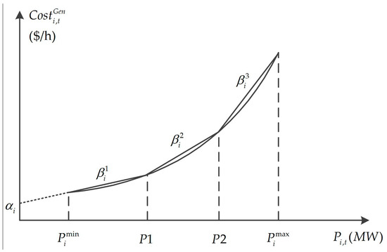
Figure 3. Linearization of the quadratic production cost function.

The incentive cost $F_{IC}$ is to encourage customers to take an active part in DRPs, while

$$F_{IC}={\displaystyle \sum _{t=1}^{24}{A}_t[D_t^0-D_t^{DR}]}$$

(36)

$F_{EC}$ is used to measure the power shortage cost caused by the forecast errors and generation outages. By adding $F_{EC}$ into the objective function, the spinning reserve will be supplied based on an internal cost analysis without any reserve limits.

$$F_{EC}={\displaystyle \sum _{t=1}^{24}VOLL\times EEN{S}_t}$$

(37)

where $VOLL$ is the value of lost load.

4.2. Constraints

The proposed model should be subject to some equality and inequality constraints.

(1)

Power balance constraint

$${\displaystyle \sum _{i=1}^{N_{Gen}}{\gamma }_{i,t}{P}_{i,t}}+W_t^F=D_t$$

(38)

(2)

Transmission flow constraint

DC power flow is used to describe the transmission flow constraint as follows:

$$F_{m-n,t}=\frac{1}{X_{m-n}}({\delta }_{m,t}-{\delta }_{n,t})$$

(39)

$$\left|F_{m-n,t}\right|\le F_{m-n}^{\max }$$

(40)

where $F_{m-n,t}$ is the line flow per $t$-th period of branch $m-n$, and $F_{m-n}^{\max }$ is the maximum limit. $X_{m-n}$ is the reactance of branch $m-n$, and ${\delta }_{m,t}$ is the voltage angle of bus $m$ at period $t$.

(3)

Power generation constraint

$$P_i^{\min }{\gamma }_{i,t}\le P_{i,t}\le P_i^{\max }{\gamma }_{i,t}$$

(41)

where $P_i^{\min }$ and $P_i^{\max }$ are minimum and maximum generation capacity of unit $i$, respectively.

(4)

On/off constraint

Once a unit is committed or shut down, it has to remain on/off for a minimum number of hours. These constraints are given as

$$\{\begin{array}{c}({\gamma }_{i,t-1}-{\gamma }_{i,t})\times (X_{i,t-1}^{on}-T_i^{on})\ge 0\\ ({\gamma }_{i,t}-{\gamma }_{i,t-1})\times (X_{i,t-1}^{off}-T_i^{off})\ge 0\end{array}$$

(42)

where $X_{i,t-1}^{on}$/$X_{i,t-1}^{off}$ are number of hours for which unit $i$ has been on/off until period $t-1$; and $T_i^{on}$/$T_i^{off}$ are minimum hours of unit $i$ has to remain on/off.

(5)

Ramping up/down constraint

$$\{\begin{array}{c}{P}_{i,t}{\gamma }_{i,t}-P_{i,t-1}{\gamma }_{i,t-1}\le P_i^{up}\\ P_{i,t-1}{\gamma }_{i,t-1}-P_{i,t}{\gamma }_{i,t}\le P_i^{down}\end{array}$$

(43)

where $P_i^{up}$ is the ramping up limit of unit $i$, and $P_i^{down}$ is the ramping down limit of unit $i$.

(6)

Reliability constraint

The reliability constraint is to ensure EENS at each period within the security level. By limiting EENS, the spinning reserve will get configured automatically to guarantee the security of power system.

$$EEN{S}_t\le EEN{S}^{\max }$$

(44)

where $EEN{S}^{\max }$ is the maximum value of EENS set by operators.

5. Case Studies and Discussion

In this section, the proposed model is tested with the modified IEEE Reliability Test System, as shown in Figure 4. This system contains 26 thermal units with capacity of 3105 MW. Those six hydro units in the initial system are replaced with a wind farm connecting to bus 14, and the total wind power capacity is 630 MW. Parameters of all thermal units and branches are taken from [36]. The forecast load and wind power are presented in Table 1. Obviously, the output of the wind farm is equipped with the anti-peak characteristic compared to the forecast load, increasing the peak-valley difference.

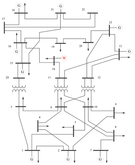
Figure 4. The modified IEEE reliability test system.

Table 1. Forecast load and wind power.

Period	Load (MW)	Wind (pu)	Period	Load (MW)	Wind (pu)
1	1901	0.845	13	2599	0.597
2	1951	0.928	14	2498	0.696
3	2050	0.923	15	2400	0.81
4	2153	0.853	16	2247	0.956
5	2198	0.82	17	2198	0.895
6	2301	0.715	18	2301	0.693
7	2350	0.498	19	2398	0.583
8	2402	0.424	20	2599	0.468
9	2498	0.338	21	2500	0.391
10	2599	0.37	22	2301	0.276
11	2649	0.193	23	2099	0.562
12	2702	0.386	24	2002	0.752

To implement DRPs, the load curve is segmented into three different periods, namely valley period (11:00 p.m.–4:00 a.m.), off-peak period (5:00 a.m.–8:00 a.m. and 2:00 p.m.–6:00 p.m.), and peak period (9:00 a.m.–1:00 p.m. and 7:00 p.m.–10:00 p.m.). Accordingly, the TOU electricity price is determined as shown in Table 2. It should be noted that the incentive-based DR is evaluated in this paper with the equal values of $P{r}_t^0$ and $P{r}_t$. The price elasticity of demand is illustrated in Table 3, extracted from [34] with some changes.

Table 2. TOU electricity price.

Load	Periods	Price ($/MWh)
Valley	23:00–4:00	46
Off-peak	5:00–8:00 14:00–18:00	96
Peak	9:00–13:00 19:00–22:00	154

Table 3. Price elasticity of demand.

Elasticity	Valley	Off-Peak	Peak
Valley	−0.08	0.03	0.034
Off-peak	0.03	−0.11	0.04
Peak	0.034	0.04	−0.19

The proposed model is coded in the MATLAB environment on a 2.50-GHz Windows-based computer with core i5 processor and 4 GB of RAM. The Gurobi 6.5.2 is a computationally efficient solver to deal with this MILP problem [37].

5.1. Effect of DR on Operation without Reliability Measures

In the current case, the EENS cost is not taken into consideration. Considering the DR model above, the incentive price has a great effect on the final results. On the one hand, if the incentive price is too low, there is no motivation for consumers to participate in DR, resulting in terrible performance of DR. On the other hand, the high incentive price will increase the cost burden on operators.

To investigate the impact of DR, five different cases are implemented here. Case 1 is the base case without considering the incentive. From Case 2 to Case 5, the maximum incentive prices are $10, $15, $20 and $25/MWh respectively.

By applying DRPs on consumers, the load curves of Cases 1–5 are represented as Figure 5. As illustrated in this figure, some consumption has been transferred from the peak period to the valley or off-peak periods due to DRPs. The higher the incentive price is, the more loads will be reduced or transferred during the peak period. Thus, several sub-peaks come into being at Hours 8, 14 and 18 with respect to the increasing incentive price.

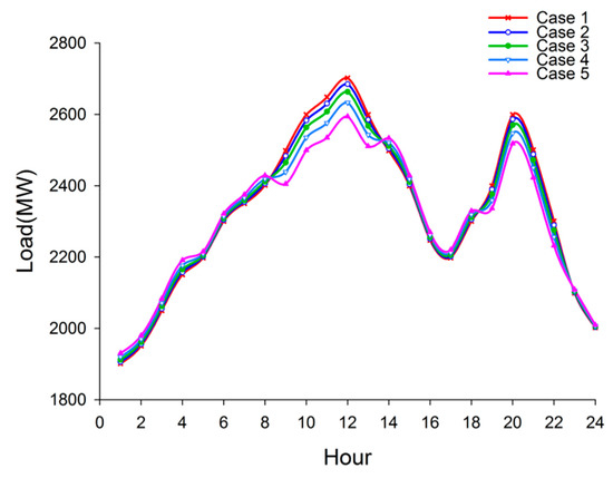
Figure 5. Comparison of load curves under different incentives.

As indicated in Table 4, the generation cost decreases as the incentive price increases. After implementing DRPs, those peak loads are reduced and transferred to the valley or off-peak periods. The load curve gets smoother so that the generators do not have to start up and shut down frequently. At the same time, the economical units will be put into production instead of those costly ones. Thus, the generation cost shows a decreasing trend along with the increasing incentive. However, another question is that the higher incentive means more fees on cost, just as shown in Table 4. Compared to the base case (Case 1), the total cost of Cases 2 and 3 have gone down. The reason is that, after implementing DRPs, the load curve has been optimized, resulting in lower generation cost. Meanwhile, increase of the incentive cost is less than decrease of the generation cost. Thus, the total cost is descending at the initial stage. Contrarily, with the incentive price rising, more compensation has to be paid to customers, giving rise to the total cost. Thus, the total cost shows a V-shaped trend of declining firstly and ascending then. According to Table 4, there should exist an optimum point located in the interval of $ (10, 15). To present the total cost trend, a few more data points are extracted every $0.5 from $10 to $15 for calculating the total cost. The incentive price can be set as a variable in the proposed model so that the optimum incentive will be obtained. By optimizing the incentive price, the optimum incentive is $12.31 while the lowest total cost is $634,706. The rough total cost trend is illustrated in Figure 6. Consequently, it is essential for operators to design the incentive price reasonably, making benefits for both sides.

Table 4. Cost comparison of Cases 1–5.

Case	Incentive Price ($/MWh)	Cost of Generation ($)	Cost of Incentive ($)	Total Cost ($)
1	0	638,919	0	638,919
2	10	633,531	1576	635,107
3	15	631,833	5318	637,151
4	20	629,133	12,605	641,738
5	25	626,405	24,620	651,025

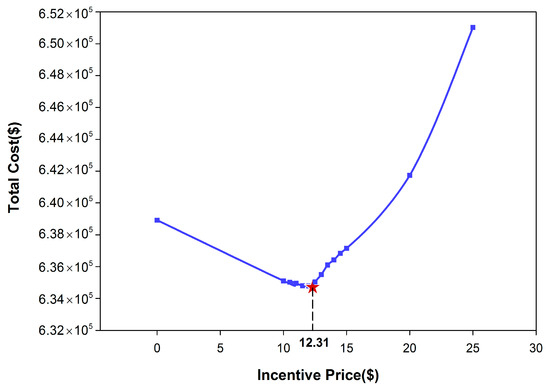
Figure 6. The total cost trend considering DR only.

5.2. Effect of DR and Reliability Measures on Operation

As mentioned above, when DRPs are considered in the day-ahead scheduling, the load curve is optimized and the total cost is able to have a little decrease. To investigate the effect of reliability measures on operation, for the first step, the objective function is modified without considering DRPs, while VOLL and EENS^max are set to $4000/MWh and 0.32 MWh. Then take both DR and reliability measures into consideration, and the incentive price is set as $10/MWh. All results are indicated in Table 5, where Case 6 is the scenario considering reliability only, and Case 7 is the scenario considering both two aspects.

Table 5. Cost comparison of cases considering DR and reliability measures.

Case	Incentive Price ($/MWh)	Cost of Generation ($)	Cost of Incentive ($)	Cost of EENS ($)	Total Cost ($)
1	0	638,919	0	0	638,919
6	0	640,531	0	24,012	664,334
2	10	633,531	1576	0	635,107
7	10	637,073	1576	23,703	662,151

Comparing Case 1 and Case 6, it can be found that the total cost $664,334 of Case 6 has been obtained. Due to reliability limits, the day-ahead scheduling is optimized, resulting in rise in the generation cost. With the addition of EENS cost, the total cost of Case 6 is $25,415 more than the base case. Similarly, the total cost of Case 7 is $27,044 more than that in Case 2. Even though there has been an increase in the cost, the security of power system is guaranteed, as shown in Table 6.

Table 6. EENS of different cases.

Case	1	6	2	7
max|EENSt| (MWh)	0.465	0.32	0.349	0.32

From another perspective, the total cost of Case 7 is less than that of Case 6. This reduction in the cost is due to the incentive-based DRPs. After implementing DR, the load curve has become smoother, resulting in decrease of cost of both generation and EENS. Thus, DR is an effective means to realize a unification of raising economy and safety.

Similarly, the optimum incentive will be determined by defining it as a variable in the proposed model. By optimizing the incentive price, the optimum incentive is $11.83 while the lowest total cost is $66,135. The total cost trend considering both DR and reliability measures is presented in Figure 7.

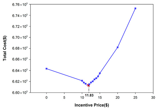
Figure 7. The total cost trend considering both DR and reliability measures.

5.3. Effect of EENS^max

In the proposed model, the reliability constraint is applied as shown in (44). Thus, in the following section, the effect of EENS^max is investigated with the range between 0.28 MWh and 0.34 MWh, while VOLL is set as $4000/MWh.

EENS and the quantities of spinning reserve under different EENS^max values are illustrated in Figure 8 and Figure 9. As the EENS^max value varies, there are sharp movements in EENS and the spinning reserve. With EENS^max decreasing from 0.34 MWh to 0.28 MWh, EENS is decreasing as well, while the spinning reserve is increasing on the contrary. This is because the lower the EENS^max value is, the more spinning reserve is required to guarantee $EEN{S}_t$ within the limit. To insure the power supply, the spinning reserve is utilized to reduce the amount of load shedding. On the other words, the EENS curves keep pace with the demand cure. The reason is that, during the peak periods, the load is heavy, leading to the decrease of the spinning reserve. The high forecast errors and outage of units may cause a great load gap, while the spinning reserve is not enough to fill in it, resulting in the rise of EENS in the peak intervals. In contrast, more spinning reserve is obtained to deal with the load gap at the valley periods. Thus, the EENS values fall off at that time.

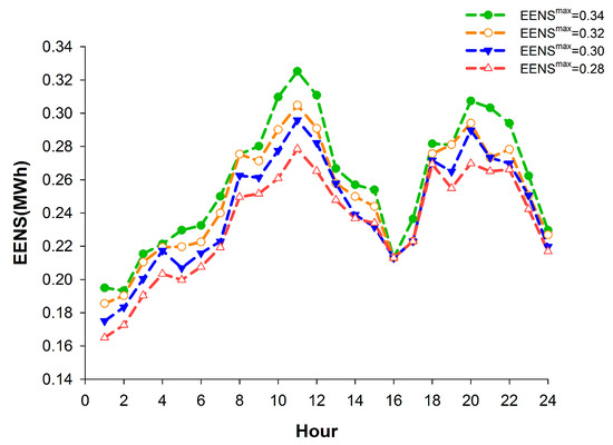
Figure 8. EENS under different EENS^max values.

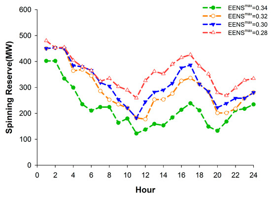
Figure 9. Spinning reserve under different EENS^max values.

In addition, it seems the spinning reserve curves show more significantly data spread at around Hour 16 where EENS are roughly the same level for different EENS^max. The reason is that, when EENS^max takes different values, the state of each unit is different as well. The smaller EENS^max is, the more units should be on to guarantee EENS^max within the constraint. At Hour 16, EENS are roughly at the same level for different EENS^max, but there still exists slight difference among them. With EENS^max decreasing from 0.34 MWh to 0.28 MWh, values of EENS are 0.2141, 0.2136, 0.2130 and 0.2128 MWh, respectively. Thus, it still presents a downward trend. On the condition of Hour 16, there are more units scheduled with the decreasing EENS^max while output of each operating unit will decrease. All these units will contribute to the value of EENS, which results in roughly the same EENS at Hour 16. The spinning reserve in this paper is defined as the difference between the overall capacity of operating units and the loads. Thus, the more operating units will provide more spinning reserve at the same load level of Hour 16. The nearly same values of EENS at Hour 16 illustrate correctness of the proposed model in this paper, which is that the stricter EENS^max is, the more spinning reserve is required for operation.

5.4. Effect of VOLL

Another important variable is VOLL, which plays a significant role in minimizing the objective function. VOLL is the value of lost load, needed to be evaluated as the average constant that consumers will lose due to the power loss of one MWh. In this part, different values of VOLL are estimated to clarify their influence on EENS and the spinning reserve.

As shown in Figure 10 and Figure 11, the quantities of EENS and the spinning reserve present two contradictory trends. When the demand level is low, the EENS level is low as well, but the spinning reserve level is high. The reason is the same with what has been explained in the previous part. Another point that should be noted is that, as the VOLL values change in three enhancing steps, the EENS is decreasing while the spinning reserve is increasing at the same period. This is because the rise of VOLL values induces a change in the equilibrium point between the cost of EENS and the spinning reserve. The higher the VOLL value is, the greater proportion the cost of EENS will take in the objective function. According to Equation (37), to minimize the total cost, the EENS value would descend indirectly when the VOLL value is increasing. Therefore, when the VOLL value is high, more spinning reserve is expected to ensure that the EENS value will keep at a low level.

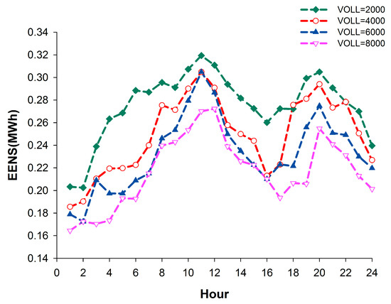
Figure 10. EENS under different VOLL values.

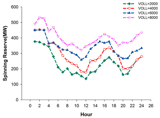
Figure 11. Spinning reserve under different VOLL values.

5.5. Effect of Possible Distributions of the Wind Power Forcast Error

Study results indicate that the practical forecast error curve of day-ahead wind power winds up faster than the Laplace distribution but slower than the Gaussian distribution [26]. Thus, the kurtosis $\kappa$ of a distribution with zero mean random error is chosen as the statistical parameter to evaluate the tail of the probability density function (PDF). The research above is based on the Gaussian PDF of the wind forecast error. In this section, the distribution of $\kappa =4.8$ between the Gaussian and Laplace PDF is extracted to form a new PDF for further research. This probability curve should be divided into seven segments as well, and detailed parameters are illustrated in Table 7.

Table 7. Parameters of seven-interval approximation with $\kappa =4.8$.

Interval	Mid-Value	Range	Probability
1	−4 ${\delta }_t^W$	[−5, −3] ${\delta }_t^W$	0.0049
2	−2.35 ${\delta }_t^W$	[−3, −1.7] ${\delta }_t^W$	0.0401
3	−1.1 ${\delta }_t^W$	[−1.7, −0.5] ${\delta }_t^W$	0.2264
4	0	[−0.5, 0.5] ${\delta }_t^W$	0.4572
5	1.1 ${\delta }_t^W$	[0.5, 1.7] ${\delta }_t^W$	0.2264
6	2.35 ${\delta }_t^W$	[1.7, 3] ${\delta }_t^W$	0.0401
7	4 ${\delta }_t^W$	[3, 5] ${\delta }_t^W$	0.0049

Replace the values of ${\epsilon }_{{\mathrm{k}}_1,\mathrm{t}}^W$ and $p_{k_1,t}$ in Section 2 with those in Table 7. The spinning reserve curves under two distributions of the Gaussian and $\kappa =4.8$ PDF are shown in Figure 12. We can see that different types of PDF have an effect on the spinning reserve. As we know, the kurtosis $\kappa$ of the Gaussian distribution is 3, i.e. smaller than 4.8. Thus, if the Gaussian PDF is adopted to simulate the forecast error of wind power, the spinning reserve will decrease, resulting in the increase of loss-of-load.

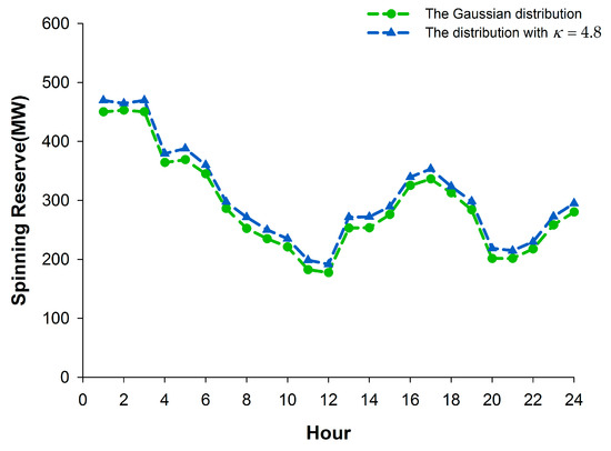
Figure 12. Comparison of the spinning reserve between the distributions of $\kappa =3$ and $\kappa =4.8$.

6. Conclusions

In this paper, a novel economic dispatch model integrating wind power is proposed, where DR and reliability measures are taken into consideration. Based on the demand vs. price elasticity and consumers’ benefit function, a modified DR model combining a dynamic incentive is introduced. Changing with variation of the different load levels at all periods, the dynamic incentive mechanism is designed to encourage customers to take an active part in peak shaving and load shifting, so that the reliability requirement of power system is satisfied. Furthermore, a new formulation of EENS is established, considering the forecast errors of wind power and load, as well as the outage replacement rate of all units. In this paper, the reliability constraint is transformed into the objective function, determining the optimal quantity of the spinning reserve by minimizing the total cost of operation. In general, the advantages of the proposed model are the following: (1) the uncertain parameters are aggregated into the EENS calculation; and (2) an optimal equilibrium point between economy and reliability of power system operation is to be obtained. The applicability of the proposed model has been illustrated through numerical studies with a modified IEEE Reliability Test System. The results demonstrate the effectiveness and practical benefits of the model above.

In future work, various DRPs and reliability measures will be taken into account to further investigate the optimization.

References

- Wei, W.; Liu, F.; Wang, J.; Chen, L.; Mei, S.; Yuan, T. Robust environmental-economic dispatch incorporating wind power generation and carbon capture plants. Appl. Energy 2016, 183, 674–684. [Google Scholar] [CrossRef]
- Shi, N.; Luo, Y. Energy Storage System Sizing Based on a Reliability Assessment of Power Systems Integrated with Wind Power. Sustainability 2017, 9, 395. [Google Scholar] [CrossRef]
- Zeng, A.; Xu, Q.; Ding, M.; Yukita, K.; Ichiyanagi, K. A classification control strategy for energy storage system in microgrid. IEEJ Trans. Electr. Electron. Eng. 2015, 10, 396–403. [Google Scholar] [CrossRef]
- Chen, H.; Zhang, R.; Li, G.; Bai, L. Economic dispatch of wind integrated power systems with energy storage considering composite operating costs. IET Generation. Tran. Dist. 2016, 10, 1294–1303. [Google Scholar] [CrossRef]
- Lei, J.; Qiao, H.; Qiu, J. Risk Assessment for Distribution Systems Using an Improved PEM-Based Method Considering Wind and Photovoltaic Power Distribution. Sustainability 2017, 9, 491. [Google Scholar]
- Osório, G.J.; Lujano-Rojas, J.M.; Matias, J.C.O.; Catalão, J.P.S. A probabilistic approach to solve the economic dispatch problem with intermittent renewable energy sources. Energy 2015, 82, 949–959. [Google Scholar] [CrossRef]
- Jiang, R.; Wang, J.; Guan, Y. Robust Unit Commitment with Wind Power and Pumped Storage Hydro. IEEE Trans. Power Syst. 2012, 27, 800–810. [Google Scholar] [CrossRef]
- Tuohy, A.; O’Malley, M. Pumped storage in systems with very high wind penetration. Energy Policy 2011, 39, 1965–1974. [Google Scholar] [CrossRef]
- Bao, Y.Q.; Li, Y.; Wang, B.; Hu, M.; Zhou, Y. Day-Ahead Scheduling Considering Demand Response as a Frequency Control Resource. Energies 2017, 10, 82. [Google Scholar] [CrossRef]
- Sekizaki, S.; Nishizaki, I.; Hayashida, T. Analysis of Electricity Market Model with Demand Response in Distribution Network. IEEJ Trans. Electr. Electron. Eng. 2015, 135, 292–303. [Google Scholar] [CrossRef]
- Siano, P. Demand response and smart grids—A survey. Renew. Sustain. Energy Rev. 2014, 30, 461–478. [Google Scholar] [CrossRef]
- Lou, S.; Lu, S.; Wu, Y.; Kirschen, D.S. Optimizing Spinning Reserve Requirement of Power System with Carbon Capture Plants. IEEE Trans. Power Syst. 2014, 30, 1056–1063. [Google Scholar] [CrossRef]
- Topić, D.; Šljivac, D.; Mandžukić, D. Influence of Different Wind Turbine Types Failures on Expected Energy Production. Available online: http://bib.irb.hr/datoteka/584067.50.pdf (accessed on 27 April 2017).
- Wang, B.; Wang, S.; Zhou, X.Z.; Watada, J. Two-stage multi-objective unit commitment optimization under hybrid uncertainties. IEEE Trans. Power Syst. 2016, 31, 2266–2277. [Google Scholar] [CrossRef]
- Koeppel, G.; Andersson, G. Reliability modeling of multi-carrier energy systems. Energy 2009, 34, 235–244. [Google Scholar] [CrossRef]
- Ramandi, M.Y.; Afshar, K.; Gazafroudi, A.S.; Bigdeli, N. Reliability and economic evaluation of demand side management programming in wind integrated power systems. Int. J. Electr. Power Energy Syst. 2016, 78, 258–268. [Google Scholar] [CrossRef]
- Yu, P.; Venkatesh, B. Fast security and risk constrained probabilistic unit commitment method using triangular approximate distribution model of wind generators. IET Gener. Tran. Dist. 2014, 8, 1778–1788. [Google Scholar] [CrossRef]
- Aghaei, J.; Amjady, N.; Baharvandi, A.; Akbari, M.A. Generation and Transmission Expansion Planning: MILP–Based Probabilistic Model. IEEE Trans. Power Syst. 2014, 29, 1592–1601. [Google Scholar] [CrossRef]
- Liu, G.; Tomsovic, K. Quantifying Spinning Reserve in Systems with Significant Wind Power Penetration. IEEE Trans. Power Syst. 2012, 27, 2385–2393. [Google Scholar] [CrossRef]
- Wang, Q.; Wang, J.; Guan, Y. Price-Based Unit Commitment with Wind Power Utilization Constraints. IEEE Trans. Power Syst. 2013, 28, 2718–2726. [Google Scholar] [CrossRef]
- Wang, Y.; Wang, B.; Chu, C.-C.; Pota, H.; Gadh, R. Energy management for a commercial building microgrid with stationary and mobile battery storage. Energy Build. 2016, 116, 141–150. [Google Scholar] [CrossRef]
- Wang, Q.; Wang, J.; Guan, Y. Stochastic Unit Commitment with Uncertain Demand Response. IEEE Trans. Power Syst. 2013, 28, 562–563. [Google Scholar] [CrossRef]
- Azizipanah-Abarghooee, R.; Golestaneh, F.; Gooi, H.B.; Lin, J.; Bavafa, F.; Terzija, V. Corrective economic dispatch and operational cycles for probabilistic unit commitment with demand response and high wind power. Appl. Energy 2016, 182, 634–651. [Google Scholar] [CrossRef]
- Çiçek, N.; Deliç, H. Demand Response Management for Smart Grids with Wind Power. IEEE Trans. Power Syst. 2015, 6, 625–634. [Google Scholar]
- Ortega-Vazquez, M.A.; Kirschen, D.S. Estimating the Spinning Reserve Requirements in Systems with Significant Wind Power Generation Penetration. IEEE Trans. Power Syst. 2009, 24, 114–124. [Google Scholar] [CrossRef]
- Kou, P.; Liang, D.; Gao, F.; Gao, L. Coordinated predictive control of dfig-based wind-battery hybrid systems: using non-gaussian wind power predictive distributions. IEEE Trans. Energy Convers 2015, 30, 681–695. [Google Scholar] [CrossRef]
- Zhang, Z.; Sun, Y.; Gao, D.; Lin, J.; Cheng, L. A Versatile Probability Distribution Model for Wind Power Forecast Errors and Its Application in Economic Dispatch. IEEE Trans. Power Syst. 2013, 28, 3114–3125. [Google Scholar] [CrossRef]
- Bludszuweit, H.; Dominguez-Navarro, J.A.; Llombart, A. Statistical analysis of wind power forecast error. IEEE Trans. Power Syst. 2008, 23, 983–991. [Google Scholar] [CrossRef]
- Bouffard, F.; Galiana, F.D. An electricity market with a probabilistic spinning reserve criterion. IEEE Trans. Power Syst. 2004, 19, 300–307. [Google Scholar] [CrossRef]
- Shu, H.; Yu, R.; Rahardja, S. Dynamic incentive strategy for voluntary demand response based on TDP scheme. In Proceedings of the Signal & Information Processing Association Summit and Conference, Hollywood, CA, USA, 3–6 December 2012; pp. 1–6. [Google Scholar]
- Lo, C.C.; Tsai, S.H.; Lin, B.S. Ice storage air-conditioning system simulation with dynamic electricity pricing: a demand response study. Energies 2016, 9, 113. [Google Scholar] [CrossRef]
- Dupont, B.; Jonghe, C.D.; Olmos, L.; Belmans, R. Demand response with locational dynamic pricing to support the integration of renewables. Energy Policy 2014, 67, 344–354. [Google Scholar] [CrossRef]
- Sahebi, M.M.; Duki, E.A.; Kia, M.; Soroudi, A.; Ehsan, M. Simultanous emergency demand response programming and unit commitment programming in comparison with interruptible load contracts. IET Gener. Trans. Dist. 2012, 6, 605–611. [Google Scholar] [CrossRef]
- Abdollahi, A.; Moghaddam, M.P.; Rashidinejad, M.; Sheikh-El-Eslami, M.K. Investigation of Economic and Environmental-Driven Demand Response Measures Incorporating UC. IEEE Trans. Smart Grid 2012, 3, 12–25. [Google Scholar] [CrossRef]
- Lee, C.; Liu, C.; Mehrotra, S.; Shahidehpour, M. Modeling Transmission Line Constraints in Two-Stage Robust Unit Commitment Problem. IEEE Trans. Power Syst. 2014, 29, 1221–1231. [Google Scholar] [CrossRef]
- Grigg, C.; Wong, P.; Albrecht, P.; Allan, R.; Bhavaraju, M.; Billinton, R.; Chen, Q.; Fong, C.; Haddad, S.; Kuruganty, S.; et al. The IEEE Reliability Test System-1996. A report prepared by the Reliability Test System Task Force of the Application of Probability Methods Subcommittee. IEEE Trans. Power Syst. 1999, 14, 1010–1020. [Google Scholar] [CrossRef]
- GUROBI 5.6, Gurobi Optimization, Inc., User’s Manual. Available online: http://gams.com/dd/docs/solvers/gurobi.pdf (accessed on 27 April 2017).
© 2017 by the authors. Licensee MDPI, Basel, Switzerland. This article is an open access article distributed under the terms and conditions of the Creative Commons Attribution (CC BY) license (http://creativecommons.org/licenses/by/4.0/).