Abstract
Urbanisation is a global trend rapidly transforming the biophysical and socioeconomic structures of metropolitan areas. To better understand (and perhaps control) these processes, more interdisciplinary research must be dedicated to the rural–urban interface. This also calls for a common reference system describing intermediate stages along a rural–urban gradient. The present paper constructs a simple index of urbanisation for villages in the Greater Bangalore Area, using GIS analysis of satellite images, and combining basic measures of building density and distance. The correlation of the two parameters and discontinuities in the frequency distribution of the combined index indicate highly dynamic stages of transformation, spatially clustered in the rural–urban interface. This analysis is substantiated by a qualitative assessment of village morphologies. The index presented here serves as a starting point in a large, coordinated study of rural–urban transitions. It was used to stratify villages for random sampling in order to perform a representative socioeconomic household survey, along with agricultural experiments and environmental assessments in various subsamples. Later on, it will also provide a matrix against which the results can be aligned and evaluated. In this process, the measures and classification systems themselves can be further refined and elaborated.
1. Introduction
Since urbanisation has been recognised as a major global challenge for the next decades, research interest in the rural–urban interface has widely increased. Although the concept of a dichotomy between interdependent “rural” and “urban” settings had a long tradition in agricultural, economic, and social sciences, scientists have become increasingly aware that there is no clear-cut border between these settings [1,2]. The space between rural and urban areas has been described as the “peri-urban or rural–urban fringe” [3,4], the “peri-urban interface” [5] or as the “rural–urban continuum” [6]. When referring to the rural–urban interface here, we include the entire region around a (mega-)city that is influenced by the growth and development of its urban core in any respect, be it infrastructurally, environmentally, economically, or socially. We presume this to be a region in which highly dynamic transitions or regime shifts occur, either by gradual adaptations, or by sudden ruptures (breakdown and restructuring [7]). Any analysis of urbanisation-related processes—and even more so interdisciplinary studies—need a method to characterise the research objects (spatial units or communities) along the interface in terms of their degree of rural versus urban character. With this in mind, the present study constructs a common reference system for a large, collaborative, interdisciplinary research project on social–ecological changes in the course of urbanisation. It aimed at drawing a representative sample of villages across the rural–urban interface of Bangalore, an emerging megacity in South India, in which subsequent surveys and field experiments shall be carried out that investigate in detail different aspects of urbanisation.
Most previous attempts to define the rural–urban interface and characterise its internal structures relied on economic, social, and political indicators and arbitrary thresholds separating different categories, such as “urban, mixed urban, mixed rural, and rural” in a rural–urban density typology [8]. Various attempts were made to replace these threshold approaches by quantitative, index-based, continuous matrices describing the degree of urbanity at any given point in an affected region.
In a study rooted in agricultural economics and aiming at a reliable baseline for rural development policies within the US, Waldorf [9] developed the “Index of relative rurality (IRR)”. It takes into account four dimensions of rurality: population size, population density, extent of urbanisation (based on demographic rather than geographic information), and remoteness. The respective derived variables were the logarithm of the population size, the logarithm of population density, the percentage of the population living in an urban area (as defined by the U.S. Census Bureau), and the distance to the closest metropolitan area, linked by calculating the unweighted average re-scaled to 0–1. That is, all the input data relied on official government statistics. The IRR is continuous, as it can take any value between 0 and 1, and comparative, as it “places the rurality of a spatial unit within the wider context of the rurality of all spatial units considered” [9] (p. 11). The IRR was determined at the county level and applied to check, e.g., for interactions of rurality with the educational profile of the population. It was later adapted to smaller scales (at the ZIP-code level) in a study directed to health care in rural areas of the US [10]. As reviewed by Beynon et al. [11], other authors used larger sets of variables and elaborate procedures of weighting and factor analysis to develop indices that capture multiple dimensions of rurality such as population and housing, migratory, and social dynamics.
Where statistical data are scarce or less available, a geographical approach based on remote sensing data may be an alternative. In a recent study a “Urban-Rural Index (URI)” was developed for two West African cities [12,13] in order to study urban and peri-urban agricultural systems. This index combines a measure of urbanisation in terms of the kernel density of existing buildings derived from high-resolution satellite imagery, and remoteness in terms of travel times to the city center, derived from extracted street networks. The construction of this index thus relies entirely on spatial structures, but requires high resolution satellite images, advanced software and advanced skills in GIS-analysis.
The index proposed in the present study follows the logic of the URI in a simplified approach, as it uses publicly accessible spatial input data such as Landsat or Sentinel satellite images provided by USGS, and open source GIS software such a QGIS. It was constructed similarly to the IRR, as an unweighted average of two normalised input variables, and shares the comparative properties of the latter. It was developed to stratify villages in the Bangalore metropolitan region by their degree of urbanity or rurality in order to draw a representative sample for a survey. Therefore, the index was termed “Survey Stratification Index (SSI)”. The need for the simplified index was thus justified by the available input data, available methods of analysis, and its intended application. The SSI, and the measures it is based on, also bear some information on the internal structure of the rural–urban interface.
The analysis was further enriched by qualitative assessment of the landscape structures around the villages and settlements, inspired by the concept of “urban morphologies” [14]. Rather than just quantifying proportions of land cover types in a given area, this approach takes into account the patterns and geometries in which different patches are arranged in space, and the related implications for land use. In particular, the approach of Gieseke et al. [14] associated certain morphologies with different agricultural production systems. In the present paper, landscape structures are analysed for patterns indicating different stages of rural–urban transitions. Synergies between quantitative and qualitative approaches are discussed.
2. Materials and Methods
Study region. In the context of a larger study which investigates social–ecological transition processes in the rural–urban interface of the South Indian metropolis, Bangalore, two transects were defined as a common space for interdisciplinary research. The Northern transect (N-transect) is a rectangular stripe of 5 km width and 50 km length, as shown in Figure 1. The lower part of this transect cuts into urban Bangalore, and the upper part contains rural villages. The Southern transect (S-transect) is a polygon covering a total area of ca. 300 km2 (Table 1).
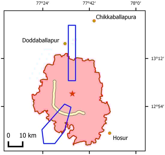
Figure 1.
Bangalore and its rural–urban interface. The red area corresponds to the districts under Bangalore’s administrative authorities. The Outer Ring Road is shown in yellow. The blue contours indicate the Northern and Southern research transects, the star marks the reference point (Vidhana Soudha) in the city centre.

Table 1.
Corner coordinates of the research transects (WGS84).
Village list and stratification unit. The list of villages and urban areas was compiled, based on the Bhuvan website [15] which was developed by the Indian Space Research Organization (ISRO) in 2009, and is a government of India satellite mapping tool similar to Google Earth and Wikimapia. The coordinates of the transects were overlaid on the Bhuvan 2D map of India to identify villages and urban areas located within the boundaries. Their names and centre point coordinates were recorded. Altogether, there were 93 villages and urban units in the N-transect and 98 in the S-transect defining the populations. In order to draw a stratified random sample from these populations, settlements were chosen as the stratification unit. This was preferred over administrative units because the classification of administrative units differs in the urban part of the transect, which is under Bangalore city administration, and is sub-divided into various wards. Since urban wards are much bigger than rural administrative villages, this would cause inconsistencies in the same sampling frame.
Stratification variable. Following the logic of the Urban–Rural Index (URI, [12]) a simplified Survey Stratification Index (SSI) was developed, whereby the simplification was twofold: in the approach of Schlesinger and Drescher [12], the dimension of building density was calculated for every image pixel as interpolated kernel density, whereas the SSI takes into account the percentage of built-up area in a defined perimeter around a village, thus cumulating over a large number of pixels. Secondly, rather than tracing travel paths along a given street network, the SSI refers to the linear distance between a village centre and the city centre. Both components, building density and distance, were investigated separately before they were combined to calculate the SSI.
Distance to the city centre. The building of the state legislature, Vidhana Soudha (12.979°N, 77.59065°E), was used as reference point for the city centre (see Figure 1). The Central Business District along MG Road and Commercial Street, as well as the racecourse, lie within a 2 km radius. WGS84 coordinates were projected into UTM 43N coordinates, and the simple linear distance from each village central point to the city centre point was measured.
Percentage of built-up area. Based on Sentinel2 satellite images of 29 April 2016 and 19 February 2016 for the Northern and Southern transect, respectively, a supervised classification was run in QGIS 2.18 to distinguish the classes of land cover: built-up, vegetation, fallow, and water. The result was then re-classified to the two classes, built-up and non-built-up.
In a first approach, the transects were subdivided in 1 km2 square grid cells, and the percentage of built-up area was calculated for each cell. When mapped as graded colours, the resulting pattern resembled the URI map of Bangalore presented in [13]. When the centre coordinates of the villages were overlaid, however, some were close to or on the cell boundaries, such that the villages could not be clearly allocated to a grid cell (not shown). In order to improve this breakdown and focus on the areas around different villages, a circular buffer zone of 1 km2 was finally defined around each village centre point, and the percentage of built-up area was determined within these circles.
Combined Survey Stratification Index (SSI). The distance to the centre and the built-up area are considered as a proxy for urbanisation. Since a high value of distance correlates to low urbanisation, whereas a high value of density indicates high urbanisation, the non-built-up area (100% minus percentage of built-up area) was used for constructing the SSI. This brings both variables to a common scale, in which low values correspond to urban character, and high values to rural character. The SSI is thus defined inversely as compared to the URI. Both the variables were normalised to a scale of 0–1 using the formula.
where, zi is the normalised variable, x is the distance or non-built-up area, min(x) is the minimum value in the transect, max(x) is the maximum value in the transect. The two measures (non-built-up area and distance) were then aggregated with equal weights to form the SSI, by calculating the geometric mean:
zi = (xi − min(x))/(max(x) − min(x))
The geometric mean was preferred over the arithmetic mean because it can accommodate extreme values and produces smoother results. The geometric mean was previously used in combining heterogeneous indices such as the Human Development Index [16], and in urbanisation vulnerability studies, such as [17,18].
Stratification and random selection of settlements. For setting optimal stratum boundaries, a variety of statistical procedures have been developed. Commonly used methods to determine stratum boundaries are the cumulative root frequency method [19], and the Lavallée–Hidiroglou iterative method [20] with Kozak’s [21] algorithm [22]. The strata boundaries constructed using these methods are listed in Table A1. In our analysis, we followed the most simple and straightforward approach and constructed six strata, which are evenly distributed over the entire range of potential SSI values by setting arbitrary boundaries at 0.167, 0.333, 0.5, 0.667, and 0.833. In total, one third of the settlements were sampled (ca. 30 out of ca. 90 per transect), whereby the number of settlements per stratum was determined in proportion to the strata size. The bigger the stratum, the higher the number of settlements selected from that stratum. This assured that the sample frame along the rural urban gradient was sufficiently representative. A lottery method without replacement was used to randomly select the settlements to be surveyed in each stratum. The complete list of villages within the research transects is provided in the Appendix A (Table A2), along with a map of the villages selected for the survey (Figure A1).
Assessment of village morphologies. In contrast to the quantitative methods of index construction and stratification described above, village morphologies are a qualitative concept. The buffer zones around all villages in the transects were visually inspected on Google Earth, and on two Worldview3 satellite images for the pattern and geometry of different land cover types. For example, rural landscapes were dominated by small compact villages surrounded by fields, whereas patchy patterns or vast empty layouts were often observed closer to the totally built-up urban area. The villages were manually assigned to one of five classes, assumed to represent different degrees of urbanisation.
Evaluation. All of the above measures were analysed for correlations and frequency distributions, and were mapped across the rural–urban interface.
3. Results
3.1. Proportion of Built-Up Area
Based on the Bhuvan map, a total of 191 villages were detected inside the defined boundaries of both transects (Figure 2). The proportion of built-up land in the 1 km2 buffer zones around these villages ranged between 1% and 89%, with an overall average of 23%.
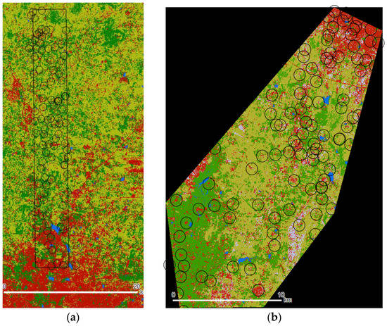
Figure 2.
Sentinel2-based land cover maps of the research areas in the rural–urban interface of Bangalore (India). (a) Northern transect and (b) Southern transect with 1 km2 buffer zones around the detected villages. Land cover classes: built-up (red), vegetation (dark green), fallow (light green), and water (blue).
In the given population, villages with ca. 10% built-up area prevailed, and the sum of the intervals around 10% and 20% made up 65% of the total number of villages (Figure 3). Local minima were around 35% and 70% built-up area.
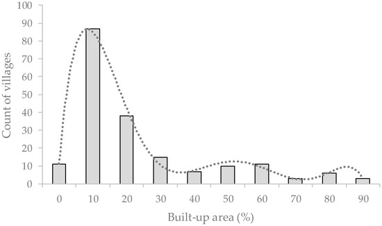
Figure 3.
Frequency distribution of villages around Bangalore (India) with different extent of built-up area (rounded to 10%).
3.2. Distances
The range of values for this parameter depends on the location and shape of the transects. In the Northern transect, the most proximal village was 9.2 km, and the most distal village 47.2 km from the urban centre (defined at Vidanha Soudha); in the Southern transect they were at 8.8 and 40.1 km, respectively. When distances are normalised, i.e., the shortest distance to city centre is set to zero and the largest distance to 100%, the results still depend on the shape of the transect, and N and S-transects are not directly comparable. In both transects, the frequency of distance values was homogeneously distributed.
3.3. Correlation of Built-Up Area and Distance
When the percentage of built-up area was plotted against the distance to the city centre, marked differences were observed between the Northern and Southern transect (Figure 4).
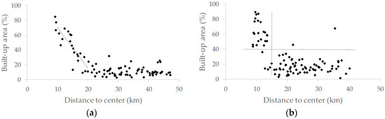
Figure 4.
Correlation of distance and percentage of built-up area in (a) the Northern and (b) the Southern research transect around Bangalore (India).
In the North, the two parameters were strongly and almost linearly (r2 = 0.748) correlated up to ca. 20 km away from the city centre: the closer to the city, the higher the percentage of built-up area. Beyond that, however, they were not correlated. Here, the average value was around 10% built-up land cover, no matter how far from the city. In the S-transect, the plotted points fell in two clusters: villages with more than 40% built-up area were located less than 15 km away from the city centre, and villages with less than 40% lay beyond that threshold (with only few exceptions). The 15 km perimeter corresponds approximately to the position of the Outer Ring Road (see Figure 1).
3.4. Survey Stratification Index, SSI
Actual values for the combined SSI ranged from 0.032 to 0.964 in the Northern, and from 0.008 to 0.948 in the Southern transect. The SSI frequency (Figure 5) has a double-peaked distribution with a local minimum around 0.3, for the separate transects, as well as the sum of both transects.
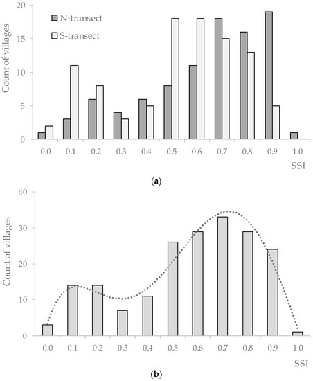
Figure 5.
Frequency distribution of villages around Bangalore (India) with different Survey Stratification Index (SSI) values, rounded to 0.1. (a) SSI calculated within each transect separately; and (b) SSI calculated taking both transects as a joint population.
When comparing the frequency distribution of the N and S transect (Figure 5a), it is noteworthy that SSI values below the urban peak are lower in the South. On the other hand, frequencies of very rural villages decrease in the South, whereas they remain rather stable in the North.
3.5. Stratification and Village Sampling
The Northern and Southern transect were treated as separate populations when calculating the SSI and allocating them to the six arbitrary strata for random sampling (Table 2; mapped in Figure A1, see Appendix A).
Table 2.
Village stratification and random sampling in the Northern and Southern transect of Bangalore (India).
As mentioned before, the SSI values of the two transects are not directly comparable due to their different shapes. If both transects were treated as a single population, and SSI was recalculated on that basis, some villages of the S-transect are classified to a neighbouring stratum (Table A3), but the overall pattern of frequency distributions as presented above remained the same.
It should be noted here, again, that the strata for the random sampling of villages were defined arbitrarily, and did not coincide with the inherent structural discontinuities indicated above. The latter, however, may give some clues to delineate areas representing urban, transitional and rural villages, as discussed below.
3.6. Landscape Structures and Village/Urban Morphologies
When examining satellite images of the transects, and in particular, the buffer zones around the villages, it was evident that there was also a change in the geometry and spatial patterns of the surface features along the transects. They reflect a morphological transition from rural characteristics (abundant in the distal parts) to urban characteristics (clustered close to the city centre). By their qualitative features, four basic classes were distinguished with a range of intermediate forms (Figure 6). In the Northern transect, 35 villages could be unambiguously described as a “compact settlement surrounded by fields” (class A, total built-up area ranged between 3% and 23%), and 24 more villages of this type showed first indications of disturbance, such as spreading out of settlements, patches of large buildings, or development of new layouts (class AB). When such disturbances outweighed the underlying pattern, a new “mixed/patchy” morphology emerged, often combined with many new layouts (class B, 15 villages, 10% to 60% built-up area), before closed, “dense settlements” prevailed which were only sparsely interrupted by green areas, such as parks, gardens, or a few residual fields (class D, 9 villages, 46% to 85% built-up area). In the Southern transect, another distinct landscape type dominated by mostly empty layouts (“all-over layouts”, class C) was encountered, which hardly ever occurred in the Northern transect. Villages per class in the Southern transect counted 26 in class A, 20 in class AB, 18 in class B, 13 in class C, and 15 in class D.
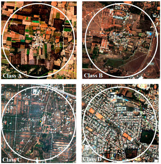
Figure 6.
Exemplary village morphologies for classes A, B, C, and D (images taken from Worldview3 scenes). The circle marks the 1 km2 buffer zone.
In order to link the qualitative morphological village description to the quantitative SSI, the frequency distribution of the morphological classes over the entire range of SSI values is shown in Figure 7. This analysis supported the existence of an urban and a rural cluster (peaks at SSI < 0.3 and SSI > 0.5, respectively), whereas the mixed/patchy type peaked between 0.3 and 0.5, that is, in the range of the local minimum observed in the SSI frequency itself (Figure 5).
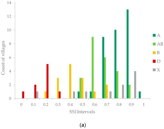
Figure 7.
Frequency distribution of morphological classes over SSI in (a) the Northern and (b) the Southern research transect around Bangalore (India). Classes: A—compact settlement surrounded by fields (rural); AB—class A with first disturbances; B—mixed/patchy; C—all-over layouts; D—dense settlements (urban); X—unclassified (unique structures or largely outside the satellite image).
In the Southern transect, this sequence was similar, with the peak of the mixed/patchy morphology shifted to slightly higher SSI values. Class C clustered in the shoulder of the urban peak, i.e., in-between classes B and D.
Although derived independently by different methods, there is obviously a correspondence between the morphological classification and the quantitative index, both representing an inherent spatial structure within the transects across the rural–urban interface.
3.7. Delineating Structural Strata
Based on the correlations, discontinuities and frequency distributions described above, the most suitable SSI thresholds for delineating a rural, transitional, and urban cluster were estimated.
In contrast to the arbitrary or statistical approaches aiming at equal SSI intervals, or at equally sized village strata, respectively, this approach takes into account the qualitative information derived from the morphological classification. The strata boundaries were adjusted to maximise the number of rural (classes A and AB), transitional (class B), and urban (classes C and D) settlements in the respective SSI interval (Figure 8). These boundaries were at 0.25 and 0.55 in the Northern transect, and at 0.35 and 0.62 in the South. Such “structural strata” might serve as a preliminary common reference for the projects targeting agronomic and ecological aspects of rural–urban transitions. Projected back on a spatial map, areas of different stages of transition can be outlined (Figure 9 and Figure 10).
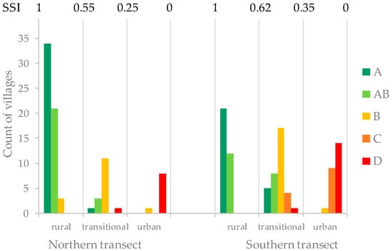
Figure 8.
Structural strata and frequency of villages within them along the rural–urban transect crossing Bangalore (India).
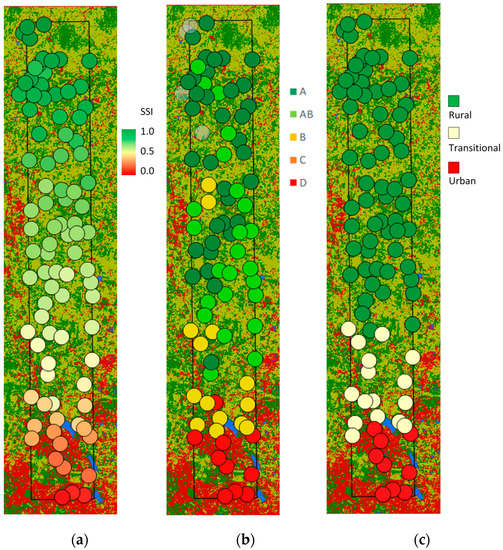
Figure 9.
Mapping of SSI, morphological classes, and structural strata in the Northern transect. (a) As the SSI is a continuous index, the transition from rural to urban character appears as a gradient in which defining boundaries is rather arbitrary; (b) The morphological classification reveals emerging hotspots of transition even in distant locations; (c) The overlay of both approaches approximates an in situ stratification in coherent rural, transitional, and urban areas.
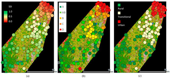
Figure 10.
Mapping of (a) SSI; (b) morphological classes; and (c) structural strata in the Southern transect. Explanations as above.
4. Discussion
4.1. Survey Stratification Index, SSI
The Survey Stratification Index (SSI) used in the present study provides a simple approach to characterising rural–urban gradients. The SSI was composed from the two variables, distance to the city centre, and proportion of built-up area around defined settlements. An initial correlation analysis of the two components revealed a breakpoint at a distance of 15 to 20 km of the city centre (Figure 4). In the Northern transect, this was a change from strong to low (or no) correlation between the two parameters, whereas in the Southern transect, it separated two clusters of different building densities. Taken together, this already suggests a transitional zone somewhere between the 15 and 20 km perimeter, where urban construction activities are most rapid. This would be an easy indicator to track city sprawl, as in the correlation analysis, landscape structures are entirely neglected. It would be interesting to analyse how this zone moves with time as the city further expands.
The classification of land cover types had some shortcomings, such as misclassification of lake edges as built-up land, which resulted in an overall accuracy of just 80%. This may be partly due to misleading ground covers, such as tank linings or plastic foil-covered fields. An independent validation for the class “built-up” was performed using 4995 points digitised from the WorldView-3 image. Here, the overall accuracy was 77%. However, in combination with the distance parameter the SSI calculation still resulted in a meaningful representation of a gradient in rural–urban features. Besides the land cover classification, the actual SSI values depend on the shape of the selected transect, and on the size of the buffer zones. The size of 1 km2 chosen here was a compromise for capturing sufficient surrounding area for a wide range of built-up area proportions, while avoiding excessive overlaps between neighbouring villages. If overlaps occurred, they were ignored in the calculation of SSI. In other landscape contexts, a suitable diameter of buffer zones might be deduced from an analysis of distances to the nearest neighbouring villages.
The use of buffer zones around a defined village centre point, however, offers two advantages. On one hand, the analysis is targeted to existing settlements rather than screening random locations, on the other hand, it averages spatial features over the given buffer area. In a suitable range of scaling, this enhances the gradient features. For example, if the buffer zones were only 1/10 of the present size (i.e., within the village limits), also the rural villages would become an almost completely built-up area, whereas a histogram over the entire image area would blur the internal discontinuities (as shown for the URI in [13] (p. 309, Figure 5). This illustrates how critical scale and resolution are for the spatial analysis of a rural–urban gradient.
The chosen boundary conditions revealed a two-peaked frequency distribution of the SSI. This suggests that the first peak, around 0.1, represents urban settlements, the other one, around 0.7, a (variety of) rural structures. The local minimum at 0.3 would then indicate an unstable stage, i.e., the villages in this SSI range should be most actively transforming. While this overall pattern was similar in both transects, lower SSI values under the urban peak in the Southern transect indicate a higher degree of urbanisation, along with higher numbers of such settlements. The decreasing frequency of very distant, rural villages in the South may be related to the influence of the neighbouring city of Kanakapura in the southern direction, which perhaps triggers construction activities from the distal end of the transect. Thus, the spatial distribution of SSI strata was somewhat irregular in the Southern transect, but rather continuous and successive in the North.
The pixel size of the Sentinel2 pictures on which the SSI calculation was based, was 10 m. The impact of lower or higher resolution of the satellite imagery (e.g., 30 m in Landsat images, or 1.24 m in Worldview3 products) merits further study. Likewise, the conclusion that the discontinuities in the correlation of distance and proportion of built-up area, or in the frequency distribution of the SSI, indicate a structurally unstable urban fringe, may be tested by time series analyses and at other locations.
4.2. Village Morphologies
Structural morphologies are a qualitative concept used in landscape and urban planning. Here, the definition of classes is entirely context specific. The WBGU has even defined a distinct dimension, termed “Eigenart” (a German word meaning “character”) [23] (p. 3) as a framework for dealing with sociocultural diversity and regional, specific development dynamics in urbanisation. Based on a careful inspection of the landscape context in the Bangalore region, it was evident that rural settlements can be described as “compact village surrounded by fields” (Class A), whereas the city centre was densely built-up, with only sparse interruptions by green areas (Class D). Class C, which is dominated by empty layouts, represents a state in which land use change (from agricultural to residential use) has already been completed but the corresponding land cover change (from open/vegetated to built-up) is still ongoing. In terms of social–ecological transitions, however, this was accounted for as “urban” rather than actively transforming. Class B, the “mixed/patchy” morphology is presumed to be most unstable. The coincidence of a local minimum in SSI frequency distribution, with a peak in the abundance of a transitional morphology (Class B), can thus be understood as a triangulation for detecting the hotspots of transformation in the rural–urban interface of Bangalore.
4.3. Other Approaches
It is obvious that our approach has qualitative elements that make it, to some degree, subjective. For example, the transitions between morphologies A and B are gradual, and it depends on the observer where to delimit a new class. This is considered in the current analysis by introducing an intermediate Class AB for villages where the “pure” radially centred symmetry shows first disturbances. Nevertheless, a subjective component persists. To overcome this bias, landscape structures can be analysed by quantitative, statistical measures, such as diversity and evenness indices [24], or by advanced landscape metrics (FRAGSTATS [25]). Salvati et al. [24], for example, used the Shannon diversity index and the Pielou index to evaluate the variability of land use classes and their contribution to the total area. They were thus able to categorise the transition from urban to rural areas for the city of Athens.
A more precise and dynamic approach for identifying the urban–rural fringe was presented by Peng et al. [26]. They developed a model which combined spatial continuous wavelet transform for the detection of mutation points from a land use degree index map with a kernel density estimation. The latter generates a density surface map from the detected mutation points, which was then used to set a threshold to produce the urban–rural fringe map. The model was successfully applied to Bejing City, and was found to be superior to manual mutation point mapping.
In an attempt to combine land cover and morphological patterns Bechtel et al. [27] adapted the Local Climate Zone mapping (originally developed for climate change research) to the analysis of urban form and function. They aim at generating a worldwide database to describe the internal structure and texture of cities, but the approach might well be extended to settlements in the rural–urban interface, and substantiate the classification suggested above.
Finally, the overall strategy followed in our present study, and in the cited examples, is not restricted to a rural–urban context. Barve et al. [28] used the combination of a composite index based on GIS analysis and ground measurement of selected ecological indicators to derive and validate threat maps in a wildlife sanctuary in Southern India. The study area was divided in 30 ha grid cells, and the GIS-based parameters were the number of villages and roads in a 3 km buffer zone around each grid cell, distance to the settlements and roads, and the average slope in and around each grid cell (all individually normalised to 0 to 1). Mapping of the weighted, composite threat index identified vulnerable zones at the edges of the sanctuary, and around plantations within it. The threat index was then used to define transects for determining ecological indicators, similar to our application of the SSI in stratifying the villages for random sampling. The ecological parameters, such as tree species richness or proportion of cut and broken stems (due to human or livestock invasion), were highly correlated with the GIS-derived threat indices.
All of the approaches discussed above aim at structuring space, and they should not be seen as exclusive of each other. Instead, they capture different facets of a research region, such as a rural–urban interface, and the method of choice will depend on the goal and the stage of a given study. The merit of the simplified index, as compared to the cited examples of more elaborate methods of analysis, lies in the swiftness of providing results, which can be easily applied in various disciplinary contexts. Furthermore, the integration of the index with the morphological classification illustrates how to overcome methodological bias between disciplines that prefer qualitative over quantitative research, or vice versa.
5. Conclusions
In the context of our project, the SSI serves as a starting point for deeper investigation in different research fields. It was applied, initially, to stratify villages for random sampling, in order to perform a representative household survey, but it will also provide a matrix against which the results can be aligned and evaluated. Coordinated research in the sampled villages, however, will not only address socioeconomic household characteristics, but also their agricultural practices in crop or dairy production, consumption practices, and attitudes to environmental issues. At the same time, experiments are carried out at selected locations to assess the actual environmental conditions, in terms of soil and crop quality, biodiversity, and provision of ecosystem services. Various rural–urban parameters, and the locations to where they map in the research transects, will thus be a central tool for synthesising interdisciplinary results. The measures and classification systems themselves will be refined and elaborated in this process, and it will be interesting to observe under which condition a numerical index, a morphology, or a location is predominant for gradients in other parameters.
Acknowledgments
This paper resulted from a collaboration of projects B02, C01, C02 and Z of the Research Unit FOR2432 (Social–Ecological Systems in the Indian Rural–Urban Interface: Functions, Scales and Dynamics of Transition). The concept of spatial explicity and of using indices to describe the internal structure of the rural–urban interface was developed jointly by the participants of FOR2432. On behalf of the entire consortium we thank the speakers, A. Bürkert and S. von Cramon-Taubadel, for inspiring discussions. We notably thank our scientific partners in DBT-FOR2432 for their collaboration and support in several excursions exploring the rural–urban interface of Bangalore, in the communication with Indian authorities and stakeholders and in the coordination of fieldwork, in particular, and on behalf of the entire Indian consortium, B.V. Chinnappa Reddy, K.N. Ganeshaiah and V.R.R. Parama at the University of Agricultural Sciences, Bangalore. We thank Eva Goldmann for performing the land cover classification and basic GIS analysis, as well as Johannes Bettin and Johannes Wegmann for supporting village extraction/mapping and ground truthing. The authors gratefully acknowledge the financial support provided by the German Research Foundation, DFG, through grant numbers BU 1308/14-1 (Z), WO 1470/3-1 (B02), KL894/23-1 (C02), and WA2135/4-1 (C01), as parts of the Research Unit FOR2432/1.
Author Contributions
In the work reported above, project C02 (Nils Nölke) provided the Sentinel2 satellite pictures on which the land cover analysis is based, and project C01 (Thomas Möckel) the Worldview3 scenes used in the village morphology classification. Thomas Möckel also prepared the maps presented in the paper. Monish Jose (B02) was responsible for drawing the stratified random sample of villages in the two transects, which included collecting information from Indian government authorities, village mapping, ground verification, mathematical definition of the SSI, choice of the stratification strategy, and contribution of the respective passages of the text. Ellen Hoffmann (Z) outlined the paper, designed the GIS analysis strategy, contributed the morphological classification, integrated and finalized the manuscript.
Conflicts of Interest
The authors declare no conflict of interest. The founding sponsors had no role in the design of the study; in the collection, analyses, or interpretation of data; in the writing of the manuscript, and in the decision to publish the results.
Appendix A. Alternative Approaches to Stratification and Random Selection of Settlements
Table A1.
Stratum boundaries determined by the cumulative root frequency method [19] and the Lavallée–Hidiroglou iterative method [20] with Kozak’s [21] algorithm [22].
Table A1.
Stratum boundaries determined by the cumulative root frequency method [19] and the Lavallée–Hidiroglou iterative method [20] with Kozak’s [21] algorithm [22].
| Transect | Strata Boundaries: Cum Root | Units in Each Stratum | Number of Units to Sample in Each Stratum | Strata Boundaries: LH | Units in Each Stratum | Number of Units to Sample in Each Stratum |
|---|---|---|---|---|---|---|
| North | <0.28 | 11 | 7 | <0.29 | 12 | 8 |
| 0.5 | 12 | 6 | 0.44 | 16 | 6 | |
| 0.64 | 16 | 6 | 0.62 | 13 | 5 | |
| 0.74 | 18 | 4 | 0.75 | 24 | 8 | |
| 0.86 | 18 | 4 | 0.85 | 16 | 3 | |
| >0.86 | 18 | 4 | >0.85 | 20 | 5 | |
| Total | 93 | 31 | 93 | 31 | ||
| South | <0.1963 | 14 | 5 | <0.1813 | 14 | 5 |
| 0.4363 | 14 | 8 | 0.3476 | 10 | 3 | |
| 0.5407 | 17 | 3 | 0.5375 | 21 | 8 | |
| 0.645 | 20 | 4 | 0.6505 | 20 | 4 | |
| 0.7598 | 17 | 4 | 0.7859 | 20 | 5 | |
| >0.7598 | 16 | 6 | >0.7859 | 13 | 5 | |
| Total | 98 | 30 | 98 | 30 |
Note: LH stands for Lavallée–Hidiroglou method of strata construction. LH method is used with Kozak’s algorithm; R: stratification package available from [29] is used for calculation.
Table A2.
List of villages within the rural–urban research transects in Bangalore, India. Sampled villages are highlighted in bold. (a) Northern transect; (b) Southern transect.
Table A2.
List of villages within the rural–urban research transects in Bangalore, India. Sampled villages are highlighted in bold. (a) Northern transect; (b) Southern transect.
| (a) Northern Transect | |||||
| Village Name | Distance (km) | Built-Up Area (%) | SSI | Stratum | Morphology Class |
| Addigandhalli | 21.56 | 18.34 | 0.516 | 4 | B |
| Adinarayanahosahalli | 33.09 | 6.63 | 0.764 | 5 | A |
| Agrahara | 22.42 | 4.31 | 0.578 | 4 | B |
| Alijenahalli | 38.41 | 3.04 | 0.861 | 6 | X |
| Allalasandra | 11.60 | 54.69 | 0.176 | 2 | D |
| Aluruguddanahalli | 32.53 | 6.42 | 0.756 | 5 | AB |
| Amruthahalli | 9.43 | 66.82 | 0.064 | 1 | D |
| Anantapura | 15.13 | 41.82 | 0.305 | 2 | B |
| Ardeshahalli | 26.97 | 12.09 | 0.641 | 4 | A |
| Atturu | 14.22 | 51.67 | 0.256 | 2 | D |
| Avalahalli | 17.49 | 35.48 | 0.377 | 3 | B |
| Ayyammanahalli | 46.59 | 9.12 | 0.942 | 6 | X |
| Bachchahalli | 30.25 | 15.44 | 0.683 | 5 | A |
| Bairadenahalli | 34.46 | 3.09 | 0.801 | 5 | A |
| Bannamangala | 31.11 | 9.75 | 0.720 | 5 | A |
| Basavanapur | 27.26 | 7.95 | 0.661 | 4 | A |
| Bettahalasur | 20.26 | 24.37 | 0.471 | 3 | AB |
| Bettanahalli | 25.37 | 7.34 | 0.628 | 4 | AB |
| Bhumenahalli | 44.22 | 9.77 | 0.908 | 6 | A |
| Bidikere | 40.45 | 6.21 | 0.875 | 6 | A |
| Byatarayapur | 9.57 | 77.42 | 0.060 | 1 | D |
| Chikka Bommasandra | 12.32 | 69.06 | 0.163 | 1 | D |
| Chikka Hegganahalli | 25.41 | 12.50 | 0.611 | 4 | AB |
| Chikka Muddenahalli | 47.16 | 6.23 | 0.964 | 6 | A |
| Chikkanahosahalli | 26.10 | 3.58 | 0.655 | 4 | A |
| Dasagondenahalli | 37.75 | 9.96 | 0.820 | 5 | A |
| Devarahalli | 28.81 | 7.19 | 0.691 | 5 | AB |
| Dinnuru | 30.84 | 6.49 | 0.729 | 5 | A |
| Gandarajapura | 39.66 | 10.98 | 0.842 | 6 | A |
| Gantiganahalli | 42.16 | 10.92 | 0.876 | 6 | A |
| Garighatta | 40.40 | 8.89 | 0.862 | 6 | A |
| Ghantiganahalli | 41.50 | 5.72 | 0.892 | 6 | AB |
| Guddadahalli | 32.33 | 18.12 | 0.704 | 5 | AB |
| Harohalli | 16.73 | 25.59 | 0.387 | 3 | B |
| Heggenahalli | 26.50 | 11.60 | 0.634 | 4 | AB |
| Hosuru | 27.48 | 15.10 | 0.638 | 4 | AB |
| Jakkuru | 11.07 | 46.38 | 0.171 | 2 | D |
| Jalige | 27.32 | 13.98 | 0.640 | 4 | AB |
| Jutnahalli | 28.81 | 5.33 | 0.698 | 5 | A |
| Kachahalli | 43.07 | 23.14 | 0.824 | 5 | A |
| Kamenahalli | 27.05 | 31.53 | 0.566 | 4 | AB |
| Kanchiganal | 39.74 | 11.08 | 0.842 | 6 | A |
| Kandasandra | 43.94 | 23.60 | 0.832 | 5 | X |
| Karanalu | 42.33 | 10.58 | 0.880 | 6 | AB |
| Kasavanahalli | 29.08 | 5.13 | 0.704 | 5 | A |
| Kenchenahalli | 15.48 | 36.81 | 0.327 | 2 | B |
| Kodihalli | 36.61 | 13.50 | 0.787 | 5 | AB |
| Konaghatta | 36.77 | 13.89 | 0.788 | 5 | A |
| Kudaragere | 22.91 | 8.63 | 0.575 | 4 | AB |
| Kuruvegere | 41.72 | 9.08 | 0.879 | 6 | A |
| Lakshmidevipur | 41.39 | 9.97 | 0.870 | 6 | X |
| Lingahiragollonalli | 30.47 | 6.84 | 0.721 | 5 | AB |
| Manchihalli | 15.04 | 13.27 | 0.370 | 3 | B |
| Maragondanahalli | 24.81 | 3.92 | 0.629 | 4 | AB |
| Maruthinagara | 14.19 | 61.08 | 0.228 | 2 | D |
| Moparahalli | 33.87 | 5.82 | 0.780 | 5 | A |
| Muddanahalli | 19.11 | 11.23 | 0.484 | 3 | AB |
| Nagadarsanahalli | 20.01 | 10.79 | 0.506 | 4 | A |
| Nagadenahalli | 33.69 | 15.38 | 0.736 | 5 | AB |
| Nagenahalli | 16.78 | 31.88 | 0.371 | 3 | B |
| Naraganahalli | 42.84 | 9.51 | 0.891 | 6 | A |
| Narasimhanahalli | 44.06 | 9.22 | 0.909 | 6 | A |
| Panditapur | 29.52 | 2.45 | 0.721 | 5 | A |
| Pedda tammanahalli | 46.02 | 6.94 | 0.946 | 6 | A |
| Puttanahalli | 14.47 | 60.22 | 0.237 | 2 | B |
| Raghunathpura | 34.18 | 24.88 | 0.700 | 5 | B |
| Rajaghatta | 38.28 | 16.05 | 0.799 | 5 | AB |
| Rajankunti | 22.71 | 21.28 | 0.530 | 4 | B |
| S(h)ivapura | 36.35 | 11.74 | 0.792 | 5 | A |
| Sadenahalli | 23.79 | 10.55 | 0.587 | 4 | AB |
| Sahakara Nagar | 9.21 | 84.96 | 0.032 | 1 | D |
| Satenahalli | 44.43 | 10.65 | 0.906 | 6 | A |
| Settahalasur | 16.59 | 33.86 | 0.362 | 3 | B |
| Singanayakanahalli | 18.79 | 30.30 | 0.421 | 3 | X |
| Sonnappanahalli | 36.02 | 8.26 | 0.802 | 5 | A |
| Sugatta | 18.26 | 9.16 | 0.468 | 3 | B |
| Sulakunte | 30.38 | 14.98 | 0.687 | 5 | AB |
| Sunaghatta | 30.91 | 7.56 | 0.726 | 5 | A |
| Sunnagaddahalli | 41.23 | 7.79 | 0.878 | 6 | A |
| Tankashahosahalli | 41.31 | 8.75 | 0.875 | 6 | A |
| Tarahunase | 22.08 | 13.68 | 0.542 | 4 | AB |
| Timmasandra_1 | 21.25 | 9.41 | 0.537 | 4 | X |
| Timmasandra_2 | 37.85 | 13.20 | 0.806 | 5 | X |
| Timmojamahalli | 42.56 | 7.06 | 0.900 | 6 | A |
| Tindlu_1 | 10.54 | 62.47 | 0.124 | 1 | X |
| Tindlu_2 | 28.13 | 8.94 | 0.673 | 5 | X |
| Tubagere | 43.68 | 25.68 | 0.817 | 5 | AB |
| Turuvanahalli | 47.04 | 9.75 | 0.944 | 6 | X |
| Varadanahalli | 30.86 | 15.78 | 0.691 | 5 | AB |
| Venkatala | 14.73 | 46.02 | 0.284 | 2 | B |
| Vobadenahalli | 32.83 | 10.85 | 0.743 | 5 | B |
| Yeddalahalli | 43.90 | 8.72 | 0.909 | 6 | A |
| Yelahanka | 13.52 | 64.86 | 0.203 | 2 | D |
| (b) Southern Transect | |||||
| Village Name | Distance (km) | Built-Up Area (%) | SSI | Stratum | Morphology Class |
| Agara | 18.90 | 24.49 | 0.493 | 3 | AB |
| Alhalli | 12.30 | 62.67 | 0.204 | 2 | C |
| Amruthnagar | 16.32 | 12.53 | 0.458 | 3 | X |
| Anjanpur | 13.35 | 50.24 | 0.268 | 2 | C |
| Arehalli | 9.27 | 60.27 | 0.075 | 1 | D |
| Badekatte | 20.96 | 9.97 | 0.591 | 4 | AB |
| Bairamangala | 31.37 | 23.24 | 0.744 | 5 | AB |
| Bannigeri | 30.28 | 15.42 | 0.762 | 5 | A |
| Betta halli kavadoddi | 28.50 | 11.97 | 0.744 | 5 | A |
| Bettarayanadoddi | 18.62 | 12.51 | 0.524 | 4 | AB |
| Bikaspur | 9.57 | 88.89 | 0.051 | 1 | D |
| Bylamaradadoddi | 19.86 | 4.20 | 0.582 | 4 | A |
| Chikkegaudanpalya | 13.71 | 12.51 | 0.370 | 3 | C |
| Choukahalli | 33.06 | 9.45 | 0.838 | 6 | A |
| Chuchgatta | 10.55 | 50.29 | 0.165 | 1 | D |
| Doddakabal | 40.07 | 14.05 | 0.927 | 6 | X |
| Doddakalsandra | 11.33 | 75.49 | 0.140 | 1 | D |
| Doddi | 17.31 | 5.57 | 0.506 | 4 | A |
| Gaddenchanpalya | 22.34 | 16.50 | 0.601 | 4 | B |
| Gadipalya | 24.57 | 18.13 | 0.642 | 4 | A |
| Ganiganpalya | 13.35 | 58.21 | 0.246 | 2 | D |
| Ganteganadoddi | 28.66 | 19.29 | 0.716 | 5 | AB |
| Gaudanapalya | 8.84 | 45.38 | 0.008 | 1 | D |
| Giriguddena Doddi | 27.09 | 11.85 | 0.718 | 5 | A |
| Gollahalli_1 | 37.11 | 0.80 | 0.948 | 6 | X |
| Gollahalli_2 | 29.25 | 18.01 | 0.732 | 5 | AB |
| Gopalpur | 22.83 | 12.04 | 0.628 | 4 | AB |
| Gulakamale | 21.37 | 25.44 | 0.547 | 4 | B |
| Guttepalya | 21.81 | 7.44 | 0.620 | 4 | B |
| Hanchipura | 28.94 | 11.70 | 0.754 | 5 | A |
| Harohalli | 35.38 | 67.05 | 0.529 | 4 | D |
| Hosahalli/Hasahalli | 12.76 | 50.43 | 0.250 | 2 | C |
| Hosur | 30.50 | 26.25 | 0.715 | 5 | A |
| Huchegaudanapalya | 24.57 | 18.49 | 0.641 | 4 | A |
| Hulagaudan Doddi | 36.47 | 22.48 | 0.828 | 5 | AB |
| Hulagaudanhalli | 36.43 | 23.80 | 0.820 | 5 | A |
| Hunchappanpalya | 11.85 | 35.54 | 0.249 | 2 | C |
| Isrolayout | 9.87 | 86.06 | 0.068 | 1 | D |
| Jettipalya | 28.20 | 12.86 | 0.735 | 5 | A |
| Kaddasikoppa | 37.46 | 24.46 | 0.832 | 5 | A |
| Kaggalhalli | 29.99 | 16.22 | 0.753 | 5 | A |
| Kaggalipura | 21.72 | 45.52 | 0.474 | 3 | B |
| Kanchigarapalya/Kunchigarapalaya | 21.01 | 15.73 | 0.573 | 4 | AB |
| Kanchugayyanadoddi | 17.39 | 14.03 | 0.485 | 3 | C |
| Karenahalli | 25.58 | 8.38 | 0.701 | 5 | AB |
| Kodipur | 9.99 | 44.79 | 0.143 | 1 | D |
| Kolaganhalli | 35.74 | 13.53 | 0.863 | 6 | A |
| Konankunte | 10.51 | 87.02 | 0.083 | 1 | D |
| Kulumepalya | 17.09 | 2.68 | 0.507 | 4 | X |
| Kumaraswamy Layout | 8.84 | 43.17 | 0.011 | 1 | D |
| Lakshmipur | 17.76 | 19.92 | 0.478 | 3 | B |
| Lingdiranahalli | 14.32 | 15.10 | 0.386 | 3 | C |
| Madigarapalya | 21.48 | 26.42 | 0.546 | 4 | B |
| Manjunath Ngara Chikkalsandra | 9.04 | 61.64 | 0.051 | 1 | D |
| Medmaranhalli | 34.34 | 13.65 | 0.840 | 6 | AB |
| Megal Gopahalli | 34.44 | 17.00 | 0.825 | 5 | A |
| Muddenhalli | 33.86 | 10.47 | 0.847 | 6 | AB |
| Mukkodalu | 25.59 | 15.87 | 0.672 | 5 | A |
| Munimarayyanadoddi | 17.70 | 12.52 | 0.498 | 3 | C |
| Muninagara | 26.25 | 8.39 | 0.715 | 5 | A |
| Nagegandanapalya | 14.82 | 20.71 | 0.390 | 3 | B |
| Nallammanadoddi | 19.98 | 9.86 | 0.567 | 4 | A |
| Narayanagurukul | 18.56 | 31.94 | 0.460 | 3 | B |
| Nayanakahalli | 24.07 | 8.57 | 0.668 | 5 | AB |
| Noukalapalya | 23.37 | 6.75 | 0.659 | 4 | A |
| Obichudahalli | 19.52 | 18.77 | 0.527 | 4 | B |
| Parasanapalya | 26.01 | 13.96 | 0.688 | 5 | A |
| Pattareddypalya | 22.59 | 21.28 | 0.589 | 4 | B |
| Perumanpalya/Peruvaiahnapalya | 31.02 | 12.02 | 0.790 | 5 | AB |
| Raghabanapalya | 12.67 | 13.68 | 0.326 | 2 | C |
| Rajanmadavu/Rachanamadu | 15.91 | 6.23 | 0.461 | 3 | AB |
| Ravugollu | 27.45 | 15.02 | 0.712 | 5 | AB |
| Saludoddi | 19.34 | 18.38 | 0.524 | 4 | B |
| Saluhanase | 20.55 | 28.80 | 0.517 | 4 | B |
| Santenahalli | 36.47 | 16.71 | 0.858 | 6 | AB |
| Shylendradoddi | 20.15 | 5.96 | 0.584 | 4 | A |
| Siddhanahallil | 38.92 | 6.83 | 0.947 | 6 | A |
| Silk farm | 15.67 | 12.01 | 0.439 | 3 | X |
| Somanahalli | 24.81 | 26.27 | 0.614 | 4 | AB |
| Subramanyapur | 10.56 | 60.96 | 0.147 | 1 | B |
| Sunkadakatte | 25.01 | 12.89 | 0.672 | 5 | X |
| Talghatpur | 13.48 | 58.05 | 0.250 | 2 | C |
| Taralu | 22.42 | 18.08 | 0.597 | 4 | B |
| Tataguni | 17.36 | 31.03 | 0.434 | 3 | B |
| Thattuguppe/Mariapura | 23.85 | 25.50 | 0.598 | 4 | AB |
| Timmaboyi doddi | 28.90 | 4.94 | 0.781 | 5 | A |
| Timmagaudanapalya/Banjarapalya | 20.39 | 5.14 | 0.593 | 4 | AB |
| Timmagaudandoddi | 31.97 | 20.63 | 0.767 | 5 | A |
| Timmayyanadoddi | 19.90 | 4.52 | 0.582 | 4 | A |
| Tipsandra | 12.34 | 44.34 | 0.250 | 2 | C |
| Turahalli | 11.40 | 52.67 | 0.197 | 2 | C |
| Udipalya | 19.45 | 33.25 | 0.476 | 3 | B |
| Uttarahalli | 9.60 | 80.75 | 0.069 | 1 | D |
| Uttarri | 20.78 | 13.50 | 0.575 | 4 | B |
| Vajarhalli | 12.74 | 61.85 | 0.219 | 2 | C |
| Vasantpur | 10.41 | 77.26 | 0.107 | 1 | D |
| Vasudevapur | 21.80 | 20.28 | 0.575 | 4 | B |
| Yalchenahalli | 9.40 | 76.43 | 0.065 | 1 | D |
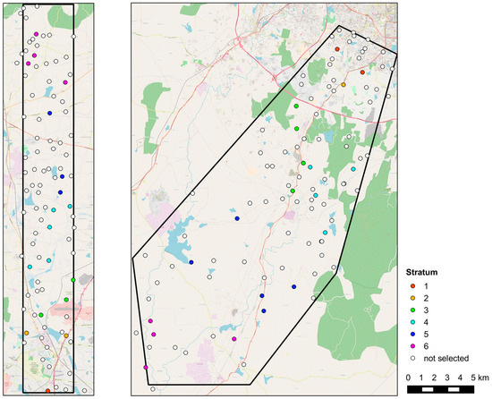
Figure A1.
Map of villages in the northern and southern transect of Bangalore (India). Villages sampled for the survey in FOR2432 are highlighted in colour. Within the selected villages the survey covered 1200 households for the general description of socio-economic parameters. Subsamples from this set are drawn for more specific investigations within various FOR2432 projects.
Stratification strategy. Due to the overall workflow and the different shapes of the two transects, the SSI values, as presented above, were determined separately. For comparison, both transects were treated as a single population, and SSI was recalculated on that basis. As a result, some villages of the S-transect were classified to a neighbouring stratum (Table A3), but the overall pattern of frequency distributions as presented above remained the same.
Table A3.
Changes in village stratification around Bangalore (India) if both transects were treated as one joint population.
Table A3.
Changes in village stratification around Bangalore (India) if both transects were treated as one joint population.
| Number of Villages | Original Stratum Allocation | Allocation after Recalculation |
|---|---|---|
| 2 | 2 | 1 |
| 1 | 3 | 2 |
| 9 | 4 | 3 |
| 13 | 5 | 4 |
| 6 | 6 | 5 |
References
- Laquinta, D.; Drescher, A.W. Defining peri-urban: Understanding rural-urban linkages and their connection to institutional contexts. In Proceedings of the 10th World Congress of the International Rural Sociology Association, Rio De Janeiro, Brazil, 30 July–5 August 2000. [Google Scholar]
- Tacoli, C. The links between rural and urban development. Environ. Urban. 2003, 15, 3–12. [Google Scholar] [CrossRef]
- Pryor, R.J. Defining the rural-urban fringe. Soc. Forces 1968, 47, 202–215. [Google Scholar] [CrossRef]
- Simon, D. Urban environments: Issues on the peri-urban fringe. Ann. Rev. Environ. Resour. 2008, 33, 167–185. [Google Scholar] [CrossRef]
- Adell, G. Theories and models of the peri-urban interface: A changing conceptual landscape. In Strategic Environmental Planning and Management for the Peri-Urban Interface Research Project; Development Planning Unit: London, UK, 1999. [Google Scholar]
- DST (Desakota Study Team). Re-Imagining the Rural-Urban Continuum: Understanding the Role Ecosystem Services Play in the Livelihoods of the Poor in Desakota Regions Undergoing Rapid Change; Institute for Social and Environmental Transition-Nepal (ISET-N): Kathmandu, Nepal, 2008. Available online: http://r4d.dfid.gov.uk/PDF/Outputs/EnvRes/FinalReport_Desakota-PartI.pdf (accessed on 16 November 2017).
- Holling, C.S. Understanding the complexity of economic, ecological, and social systems. Ecosystems 2001, 4, 390–405. [Google Scholar] [CrossRef]
- Isserman, A.M. In the national interest: Defining rural and urban correctly in research and public policy. Int. Reg. Sci. Rev. 2005, 28, 465–499. [Google Scholar] [CrossRef]
- Waldorf, B.S. A Continuous multi-dimensional measure of rurality: Moving beyond threshold measures. In Proceedings of the Annual Meeting of the American Agricultural Economics Association, Long Island, CA, USA, 24–27 July 2006; Available online: http://purl.umn.edu/21383 (accessed on 16 November 2017).
- Inagami, S.; Gao, S.; Karimi, H.; Shendge, M.M.; Probst, J.C.; Stone, R.A. Adapting the Index of Relative Rurality (IRR) to estimate rurality at the ZIP code level: A rural classification system in health services research. J. Rural Health 2016, 32, 219–227. [Google Scholar] [CrossRef] [PubMed]
- Beynon, M.J.; Crawley, A.; Munday, M. Measuring and understanding the difference between urban and rural areas. Environ. Plan. B Plan. Des. 2015, 43, 1136–1154. [Google Scholar] [CrossRef]
- Schlesinger, J.; Drescher, A. Agriculture along the urban–rural continuum: A GIS-based analysis of spatiotemporal dynamics in two medium-sized African cities. Freibg. Geogr. Hefte 2013, 70. Available online: https://www.geographie.uni-freiburg.de/publikationen/abstracts/fgh70-en (accessed on 16 November 2017).
- Schlesinger, J. Using crowd-sourced data to quantify the complex urban fabric—OpenStreetMap and the Urban–Rural Index. In OpenStreetMap in GIScience, Lecture Notes in Geoinformation and Cartography; Jokar Arsanjani, J., Zipf, A., Mooney, P., Helbich, M., Eds.; Springer: Basel, Switzerland, 2015; pp. 295–315. [Google Scholar] [CrossRef]
- Giseke, U.; Kasper, C.; Mansour, M.; Moustanjidi, Y. E1 Connecting spheres: Urban agriculture as a multidimensional strategy: E1.4 Nine urban-rural morphologies. In Urban Agriculture for Growing City Regions. Connecting Urban-Rural Spheres in Casablanca; Giseke, U., Gerster-Bentaya, M., Helten, F., Kraume, M., Scherer, D., Spars, G., Amraoui, F., Adidi, A., Berdouz, S., Chlaida, M., et al., Eds.; Routledge: Abingdon, UK; New York, NY, USA, 2015; pp. 316–328. ISBN 978-0415825016. [Google Scholar]
- ISRO. Bhuvan: Indian Geo-Platform of ISRO. Available online: http://bhuvan.nrsc.gov.in/state/KA (accessed on 4 October 2016).
- Ravallion, M. Troubling tradeoffs in the Human Development Index. J. Dev. Econ. 2012, 99, 201–209. [Google Scholar] [CrossRef]
- Qiu, B.; Li, H.; Zhou, M.; Zhang, L. Vulnerability of ecosystem services provisioning to urbanization: A case of China. Ecol. Indic. 2015, 57, 505–513. [Google Scholar] [CrossRef]
- Huang, Y.; Li, F.; Bai, X.; Cui, S. Comparing vulnerability of coastal communities to land use change: Analytical framework and a case study in China. Environ. Sci. Policy 2012, 23, 133–143. [Google Scholar] [CrossRef]
- Dalenius, T.; Hodges, J.L., Jr. Minimum variance stratification. J. Am. Stat. Assoc. 1959, 54, 88–101. [Google Scholar] [CrossRef]
- Lavallee, P.; Hidiroglou, M.A. On the stratification of skewed populations. Surv. Methodol. 1988, 14, 33–43. [Google Scholar]
- Kozak, M. Optimal stratification using random search method in agricultural surveys. Stat. Transit. 2004, 6, 797–806. [Google Scholar]
- Er, S. Comparison of the efficiency of the various algorithms in stratified sampling when the initial solutions are determined with geometric method. Int. J. Stat. Appl. 2012, 2, 1–10. [Google Scholar] [CrossRef]
- WBGU–Wissenschaftlicher Beirat der Bundesregierung Globale Umweltveränderungen. Der Umzug der Menschheit: Die Transformative Kraft der Städte; WBGU: Berlin, Germany, 2016; Available online: http://www.wbgu.de/en/hg2016 (accessed on 16 November 2017).
- Salvati, L.; Sateriano, A.; Saradakou, E.; Grigoriadis, E. ‘Land-use mixité’: Evaluating urban hierarchy and the urban-to-rural gradient with an evenness-based approach. Ecol. Indic. 2016, 70, 35–42. [Google Scholar] [CrossRef]
- McGarigal, K.; Cushman, S.A.; Ene, E. FRAGSTATS V4: Spatial Pattern Analysis Program for Categorical and Continuous Maps, version 4; Computer Software Program Produced by the Authors at the University of Massachusetts; University of Massachusetts: Amherst, MA, USA, 2012; Available online: http://www.umass.edu/landeco/research/fragstats/fragstats.html (accessed on 16 November 2017).
- Peng, J.; Zhao, S.; Liu, Y.; Tian, L. Identifying the urban-rural fringe using wavelet transform and kernel density estimation: A case study in Beijing City, China. Environ. Model. Softw. 2016, 83, 286–302. [Google Scholar] [CrossRef]
- Bechtel, B.; Alexander, P.J.; Böhner, J.; Ching, J.; Conrad, O.; Feddema, J.; Mills, G.; See, L.; Stewart, I. Mapping local climate zones for a worldwide database of the form and function of cities. ISPRS Int. J. GeoInf. 2015, 4, 199–219. [Google Scholar] [CrossRef]
- Barve, N.; Kiran, M.C.; Vanaraj, G.; Aravind, N.A.; Rao, D.; Uma Shaanker, R.; Ganeshaiah, K.N.; Poulsen, J.G. Measuring and mapping threats to a wildlife sanctuary in Southern India. Conserv. Biol. 2005, 19, 122–130. [Google Scholar] [CrossRef]
- Stratification: Univariate Stratification of Survey Populations. Available online: https://cran.r-project.org/web/packages/stratification/index.html (accessed on 13 February 2017).
© 2017 by the authors. Licensee MDPI, Basel, Switzerland. This article is an open access article distributed under the terms and conditions of the Creative Commons Attribution (CC BY) license (http://creativecommons.org/licenses/by/4.0/).