Neimark–Sacker Bifurcation Analysis and 0–1 Chaos Test of an Interactions Model between Industrial Production and Environmental Quality in a Closed Area

Abstract

A discrete-time model is presented to describe the complex interaction between industrial production and environmental quality in a closed area. Its Neimark–Sacker bifurcation and chaos are discussed based on Wen's explicit Neimark–Sacker bifurcation criterion, Kuznetsov's normal form method and center manifold theory and Gottwald and Melbourne's 0–1 test algorithm. Numerical simulations are employed to validate the main results of this work.

1. Introduction

In the handicraft economy, manufacturing was often done in people's homes or small and rural shops by using hand tools or basic machines, and life for the average person was difficult, with meager incomes and malnourishment. In that period, the environment was a utopia, almost free from human disturbance, so the pollution risk to the environment was really quite negligible, and thus, the ecological environment's capability of self-adjustment and restoration was quite strong. In contrast, after the Industrial Revolution, people produced the bulk of their own food, clothing, furniture and tools by using new chemical manufacturing and iron production processes, improving the efficiency of water power, increasing the use of steam power and developing machine tools. Unfortunately, industrial production can produce many forms of pollution as follows: air pollution, light pollution, littering, noise pollution, soil contamination, radioactive contamination, thermal pollution, visual pollution, water pollution, plastic pollution and others, increasing the risk of various occupational hazards, such as asbestosis and pneumoconiosis. Though the industrial production brought about such a greater volume and variety of industrial goods and improved the living quality for many people, particularly for the middle and upper classes, the poor and working classes were lowly paid and struggling to improve their dangerous and monotonous working conditions. What is more, they could enjoy less blessings poured out from industrial production, but suffer more from industrial pollutants than the middle and upper classes. From this point of view, studying the interactions between industrial production and environmental quality would be helpful to promoting their harmonious development, on the one hand, and improving social equity and preventing the gap between the rich and the poor from widening, on the other hand.

Based on the interaction between product and environment, Salomone et al. [1,2,3] proposed their pioneering work, the product-oriented environmental management system (POEMS), a sustainable management framework. To address the complex relationship adequately, many researchers employed various appropriate theoretical frameworks to represent the nexus between industrial production and environmental quality. For example, Zhao et al. [4] proposed a plant-level aggregation method to estimate the relationship between production's spatial distribution and regional water environmental carrying capacity in a a small region. Aşıcı [5] explored the relationship between economic growth and the pressure on nature from the environmental sustainability perspective. Dinda [6], Copeland and Taylor [7] investigated the relationship between environmental degradation and economic development. Paraschiv [8] discovered relationships between the textile industry and sustainable development and conducted a Holt–Winters forecasting investigation for the eastern European area. Empirical methods were adopted in the above research. By using differential equations, Aliehyaei et al. [9] reported the results of exergy, economic and environmental analyses of simple and combined heat and power internal combustion engines. In this paper, difference equations and numerical simulations will be employed to discover complex interactions between industrial production and environmental quality in a closed area.

As a kind of dynamical bifurcation, Neimark–Sacker bifurcation [10,11,12] is a crucial phenomenon that has drawn considerable attention in many discrete-time systems, such as financial systems [13], investment competition models [14] and Hénon systems [15]. The Neimark–Sacker bifurcation emerges with a closed invariant curve from a fixed point in discrete-time dynamical systems, when the fixed point changes stability via a pair of complex eigenvalues with unit modulus [10]. We will focus on the existence, stability and direction of Neimark–Sacker bifurcation in the interaction system.

Gottwald and Melbourne [16] firstly proposed the 0–1 test algorithm, a reliable and efficient binary test method for chaos, which is one of the simplest and most effective ones, though there have been many methods for detecting chaotic attractors. The 0–1 test algorithm has already been successfully implemented in various discrete or continuous systems, such as in [17,18,19,20,21,22,23,24,25].

The remainder of this paper is organized as follows. In Section 2, we formulate the model of the interaction between production and environment in a closed area. In Section 3, we analyze the stabilities of the real-valued fixed point of the model. In Section 4, we study the existence of Neimark–Sacker bifurcation by using Wen's Neimark–Sacker bifurcation criterion [11], and prove the stability and direction of Neimark–Sacker bifurcation by means of Kuznetsov's normal form method and center manifold theory [10]. In Section 5, we detect the chaos by using the 0–1 test algorithm [16]. Finally, the conclusion in Section 6 closes the paper.

2. Model

In this section, we focus on depicting a complex interaction between production and environment in a closed area by using nonlinear dynamics. For the purpose of our description of the model, let us first give some notations and assumptions as follows.

2.1. Notations

The following notations in Table 1 are used throughout this paper:

Table 1. Notations.

Variables/Parameters	Descriptions
$x_n$	the environmental quality index at period n;
$\left(x_{n+1}-x_n\right)$	indicates the change of environmentalquality, either improvement or deterioration;
$y_n$	the production amount at period n;
$\left(y_{n+1}-y_n\right)$	indicates the change of production amount, which represents a production decision, either an increase or a decrease;
a	the low threshold of environmental quality;
c	the high threshold of environmental quality;
b	the payment on the pollution emission right;
δ	the step size of a decision or measurement;
ϵ	a general, small parameter.

Table 1. Notations.

Variables/Parameters	Descriptions
$x_n$	the environmental quality index at period n;
$\left(x_{n+1}-x_n\right)$	indicates the change of environmentalquality, either improvement or deterioration;
$y_n$	the production amount at period n;
$\left(y_{n+1}-y_n\right)$	indicates the change of production amount, which represents a production decision, either an increase or a decrease;
a	the low threshold of environmental quality;
c	the high threshold of environmental quality;
b	the payment on the pollution emission right;
δ	the step size of a decision or measurement;
ϵ	a general, small parameter.

2.2. Assumptions

The following assumptions in Table 2 are available throughout this paper:

Table 2. Assumptions.

Assumptions	Descriptions	Expressions
Assumption 1	The environmental quality has a positive linear impact on the production decision.	$\left(y_{n+1}-y_n\right)\propto x_n$
Assumption 2	The last production amount has a negative linear impact on the current production decision due to congestion in the product market.	$\left(y_{n+1}-y_n\right)\propto -y_n$
Assumption 3	The payment on the pollution emission right has a negative linear impact on the production decision.	$\left(y_{n+1}-y_n\right)\propto -b$
Assumption 4	The production amount has a negative linear impact on the change of environmental quality.	$\left(x_{n+1}-x_n\right)\propto -y_n$
Assumption 5	The change of environmental quality is affected simultaneously by the last environmental quality and deviations from its low and high thresholds.	$\left(x_{n+1}-x_n\right)\propto x_n\left(x_n-a\right)\left(c-x_n\right)$

Table 2. Assumptions.

Assumptions	Descriptions	Expressions
Assumption 1	The environmental quality has a positive linear impact on the production decision.	$\left(y_{n+1}-y_n\right)\propto x_n$
Assumption 2	The last production amount has a negative linear impact on the current production decision due to congestion in the product market.	$\left(y_{n+1}-y_n\right)\propto -y_n$
Assumption 3	The payment on the pollution emission right has a negative linear impact on the production decision.	$\left(y_{n+1}-y_n\right)\propto -b$
Assumption 4	The production amount has a negative linear impact on the change of environmental quality.	$\left(x_{n+1}-x_n\right)\propto -y_n$
Assumption 5	The change of environmental quality is affected simultaneously by the last environmental quality and deviations from its low and high thresholds.	$\left(x_{n+1}-x_n\right)\propto x_n\left(x_n-a\right)\left(c-x_n\right)$

2.3. Model Formulation

Based on Assumptions 1–5, if we let $c=1$ and readjust the dimensions of the production amount and the environmental quality index, then we can get the following equations:

$$\left\{\begin{array}{cc}\hfill x_{n+1}-x_n& =\text{δ}(x_n(x_n-a)(1-x_n)-y_n)\hfill \\ \hfill y_{n+1}-y_n& =\text{δ}(x_n-y_n-b)\hfill \end{array}\right.$$

(1)

where $a,b,\text{δ}>0$

As we know, in some cases, x changes more quickly than y; in other cases, x changes more slowly than y. Therefore, we can employ a general small parameter ϵ to proportionally synchronize x and y as follows:

$$\left\{\begin{array}{cc}\hfill x_{n+1}& =x_n+\text{δ}(x_n(x_n-a)(1-x_n)-y_n)\hfill \\ \hfill y_{n+1}& =y_n+ϵ\text{δ}(x_n-y_n-b)\hfill \end{array}\right.$$

(2)

where $ϵ>0$.

Case 1 :$ϵ=0$.

This means that $y_{n+1}=y_n$, i.e., the production amount is a constant, for instance, because production resources are rigidly constrained or regulated by their government.

Case 2 :$0<ϵ<1$.

This means that x is a fast variable and y is a slow variable, for instance, because the environmental quality can projectively change in accordance to the producers' production amounts, whereas producers cannot change instantaneously their production amounts in a centrally-planned economy.

Case 3 :$ϵ=1$.

This means that x and y are completely synchronized. More prosaically, x and y have the same step size of decision or measurement.

Case 4 :$ϵ>1$.

This means that x is a slow variable and y is a fast variable, for instance, because the environmental quality changes gradually under government control, whereas producers can instantaneously and independently adjust their production amounts in a market economy.

3. Stability of the Fixed Points

The fixed points of system Equation (2) satisfy the following equations:

$$\left\{\begin{array}{cc}\hfill x& =x+\text{δ}\left(x\right(x-a\left)\right(1-x)-y)\hfill \\ \hfill y& =y+ϵ\text{δ}(x-y-b)\hfill \end{array}\right.$$

(3)

which have only a real-valued fixed point $E_0=(x_0,y_0)$, where:

$$\begin{array}{c}{y}_0=x_0-b\hfill \\ x_0=\frac{1+a}{3}+\frac{\sqrt[3]{2}(2+a-a^2)}{3K}-\frac{K}{3\sqrt[3]{2}}\hfill \\ K=\sqrt[3]{7+12a+3a^2-2a^3+KK-27b}\hfill \\ KK=\sqrt{4{(2+a-a^2)}^3+{(7+12a+3a^2-2a^3-27b)}^2}\hfill \end{array}$$

The Jacobian matrix of system Equation (2) at $E_0$ is given by:

$$J\left(E_0\right)=\left(\begin{array}{cc}KA& -\text{δ}\\ \text{δ}ϵ& 1-\text{δ}ϵ\end{array}\right)$$

(4)

where $KA=1+\text{δ}((x_0-a)(1-x_0)+x_0(1-x_0)-x_0(x_0-a))$. Its characteristic equation can be written as:

$$p\left(\lambda \right)={\lambda }^2+p_1\lambda +p_2=0$$

(5)

where:

$$\begin{array}{c}{p}_2=\text{δ}(a-2x_0-2a{x}_0+ϵ+3x_0^2)-2\hfill \\ p_1={ϵ\text{δ}}^2(a+1-2x_0+3x_0^2-2a{x}_0)-1-p_2\hfill \end{array}$$

According to the relations between roots and coefficients of a quadratic equation, one can get the following proposition.

Proposition 1.

Let $p\left(\lambda \right)={\lambda }^2+p_1\lambda +p_2$. Suppose that $p\left(1\right)>0$, ${\lambda }_1$ and ${\lambda }_2$ are two roots of $p\left(\lambda \right)=0$. Then, the fixed point $E_0$ is:

(i)

locally asymptotically-stable if and only if$p(-1)>0$and$p_2<1$;

(ii)

a saddle if and only if $p(-1)<0$;

(iii)

locally unstable if and only if $p(-1)>0$ and $p_2>1$;

(iv)

non-hyperbolic if either $p(-1)=0$ and $p_1\ne 0,2$ or $p_1^2-4p_2<0$ and $p_2=1$.

4. Neimark–Sacker Bifurcation

4.1. Existence of Neimark–Sacker Bifurcation

In order to discuss the existence of Neimark–Sacker bifurcation, an explicit criterion of Neimark–Sacker bifurcation needs to be introduced as follows.

Lemma 1.

[11] For an n-th order discrete-time dynamical system, assume first that at the fixed point $x_0$, its characteristic polynomial of Jacobian matrix $A={\left(a_{ij}\right)}_{n\times n}$ takes the following form:

$$\begin{array}{c}\hfill p_{\text{μ}}\left(\lambda \right)={\lambda }^n+a_1{\lambda }^{n-1}+\cdots +a_{n-1}\lambda +a_n\end{array}$$

where $a_j=a_j(\text{µ},k),j=1,\cdots ,n,$ µ is the bifurcation parameter and k is the control parameter or the other to be determined. Consider the sequence of determinants${△}_0^{\pm }(\text{µ},k)=1,{△}_1^{\pm }(\text{µ},k),\cdots ,{△}_n^{\pm }(\text{µ},k),$where:

$${△}_j^{\pm }(,k)=\left|M_1\pm M_2\right|,j=1,\cdots ,n$$

where:

$$M_1=\left(\begin{array}{ccccc}1& a_1& a_2& \cdots & a_{j-1}\\ 0& 1& a_1& \cdots & a_{j-2}\\ 0& 0& 1& \cdots & a_{j-3}\\ \cdots & \cdots & \cdots & \cdots & \cdots \\ 0& 0& 0& \cdots & 1\end{array}\right)M_2=\left(\begin{array}{ccccc}{a}_{n-j+1}& a_{n-j+2}& \cdots & a_{n-1}& a_n\\ a_{n-j+2}& a_{n-j+3}& \cdots & a_n& 0\\ \cdots & \cdots & \cdots & \cdots & \cdots \\ a_{n-1}& a_n& \cdots & 0& 0\\ a_n& 0& \cdots & 0& 0\end{array}\right)$$

If the following conditions hold,

(H1) 

Eigenvalue assignment ${△}_{n-1}^{-}({\text{μ}}_0,k)=0,$ $p_{{\text{μ}}_0}\left(1\right)>0,$ ${(-1)}^n{p}_{{\text{μ}}_0}(-1)>0,$ ${△}_{n-1}^{+}({\text{μ}}_0,k)>0,$${△}_j^{\pm }({\text{μ}}_0,k)>0,$$j=n-3,n-5,\cdots ,1\left(or2\right),$ when n is even (or odd, respectively),

(H2) 

Transversality condition $d{△}_{n-1}^{-}({\text{μ}}_0,k)/d\text{μ}\ne 0,$

(H3) 

Non-resonance condition $cos(2\pi /m)\ne \psi$ or resonance condition $cos(2\pi /m)=\psi$, where $m=3,4,5,\cdots$ and $\psi =1-0.5p_{{\text{μ}}_0}\left(1\right){△}_{n-3}^{-}({\text{μ}}_0,k)/{△}_{n-2}^{+}({\text{μ}}_0,k),$ then a Neimark–Sacker bifurcation occurs at ${\text{μ}}_0$.

According to Lemma 1, for $n=2$, we can get the following equalities and inequalities:

$${▵}_1^{-}\left(ϵ\right)=\left|1-p_2\right|=0$$

(6)

$$p_{ϵ}\left(1\right)=1+p_1+p_2>0$$

(7)

$${(-1)}^2{p}_{ϵ}(-1)=1-p_1+p_2>0$$

(8)

$${▵}_1^{+}\left(ϵ\right)=\left|1+p_2\right|>0$$

(9)

$$\begin{array}{c}\hfill d{△}_1^{-}({ϵ}_0,k)/d\epsilon =a\text{δ}-2\text{δ}{x}_0-2a\text{δ}{x}_0+ϵ\text{δ}+3\text{δ}{x}_0^2-2\ne 0\end{array}$$

(10)

By using the Mathematics software to solve Equations (6)–(10), the critical value of Neimark–Sacker bifurcation of system Equation (2) can be obtained as the two following expressions:

$$\left(i\right){\text{δ}}^{*}=\frac{2a{x}_0+2x_0-3x_0^2-a-ϵ}{ϵ(2a{x}_0+2x_0-3x_0^2-a-1)}$$

(11)

when $(x_0>\frac{1}{2}\cap K_1>a\cap ϵ<K_2+K_3\cap ϵ>K_2-K_3)\cup (x_0<\frac{1}{2}\cap K_1<a\cap ϵ<K_2+K_3\cap ϵ>K_2-K_3)$ holds.

$$\left(ii\right){ϵ}^{*}=\frac{2a{x}_0+2x_0-3x_0^2-a}{2a\text{δ}{x}_0-3\text{δ}{x}_0^2-a\text{δ}+2\text{δ}{x}_0-\text{δ}+1}$$

(12)

when $(x_0>\frac{1}{2}\cap K_1>a\cap <K_4-K_5\cap ϵ>-K_4-K_5)\cup (x_0<\frac{1}{2}\cap K_1<a\cap <K_4-K_5\cap ϵ>-K_4-K_5)$ holds, where $K_1=\frac{1-2x_0+3x_0^2}{-1+2x_0},K_2=2+a-2x_0-2a{x}_0+3x_0^2,K_3=2\sqrt{K_2-1},K_4=2{\left((K_2-1){(2-K_2)}^2\right)}^{-\frac{1}{2}},K_5=\frac{2}{2-K_2}.$

Thus, it follows from Equation (1) that the eigenvalues satisfy the condition (H1) in Lemma 1, that is Neimark–Sacker bifurcation occurs at the fixed point $E_0=(x_0,y_0)$.

4.2. Direction and Stability of the Neimark–Sacker Bifurcations

In this section, we will use Kuznetsov’s normal form method and center manifold theory [10] to investigate the direction and stability of the Neimark–Sacker bifurcations in the system Equation (2). Since the fixed point $E_0=(x_0,y_0)$ is not origin $O(0,0)$, the $E_0$ need to be transformed to the origin by the following change of variables:

$$x=x_0+u,y=y_0+v$$

This transforms system Equation (2) into the following equivalent system:

$$\left\{\begin{array}{cc}\hfill u_{n+1}=& u_n+x_0+\text{δ}((u_n+x_0)(u_n+x_0-a)(1-u_n-x_0)-v_n-y_0)\hfill \\ \hfill v_{n+1}=& v_n+y_0+ϵ\text{δ}(u_n+x_0-b-v_n-y_0)\hfill \end{array}\right.$$

(13)

This system can be written as:

$$\begin{array}{c}\hfill X_{n+1}=J{X}_n+\frac{1}{2}B(X_n,X_n)+\frac{1}{6}C(X_n,X_n,X_n)+O\left(X_n^4\right)\end{array}$$

where $X_n={\left(u_n,v_n\right)}^T$ is the vector of the transformed system and J is the Jacobin matrix of systemEquation (11) evaluated at the origin $O(0,0)$ as follows.

$$J\left(O\right)=\left(\begin{array}{cc}KA& -\text{δ}\\ \text{δ}ϵ& 1-\text{δ}ϵ\end{array}\right)$$

(14)

Additionally, the multilinear functions $B:{\text{ℝ}}^2\times {\text{ℝ}}^2\to {\text{ℝ}}^2$ and $C:{\text{ℝ}}^2\times {\text{ℝ}}^2\times {\text{ℝ}}^2\to {\text{ℝ}}^2$ are defined respectively by:

$$B_i(x,y)=\sum _{j,k=1}^n\frac{{\partial }^2{X}_i(\xi ,0)}{\partial {\xi }_j\partial {\xi }_k}{|}_{\xi =0}{x}_j{y}_k,i=1,2$$

$$C_i(x,y,z)=\sum _{j,k,l=1}^n\frac{{\partial }^3{X}_i(\xi ,0)}{\partial {\xi }_j\partial {\xi }_k\partial {\xi }_l}{|}_{\xi =0}{x}_j{y}_k{z}_{l}i=1,2$$

which take on the planar vectors $\xi ={({\xi }_1,{\xi }_2)}^T$, $\text{η}={({\text{η}}_1,{\text{η}}_2)}^T$ and $\text{ζ}={({\text{ζ}}_1,{\text{ζ}}_2)}^T$.

For the system Equation (13),

$$B(\xi ,\text{η})=\left(\begin{array}{c}(2a-6x_0+2)\text{δ}{\xi }_1{\text{η}}_1\\ 0\end{array}\right)$$

$$C(\xi ,\text{η},\text{ζ})=\left(\begin{array}{c}-6\text{δ}{\xi }_1{\text{η}}_1{\text{ζ}}_1\\ 0\end{array}\right)$$

The eigenvalues of the matrix $J\left(O\right)$ are:

$${\lambda }_{1,2}=N_0\pm i\frac{1}{2}\sqrt{N_1}=e^{\pm i_0}$$

(15)

where:

$$\begin{array}{c}{N}_0=1+\text{δ}{x}_0+a\text{δ}{x}_0-\frac{1}{2}\left(a\text{δ}+\text{ϵ}\text{δ}+3\text{δ}{x}_0^2\right)\hfill \\ N_1={-\text{δ}}^2\left(4N_2{x}_0+2N_3{x}_0^2+3N_4{x}_0^3-N_5\right)\hfill \\ N_2=a\text{ϵ}+\text{ϵ}-a-a^2\hfill \\ N_3=2-3\text{ϵ}+7a+2a^2\hfill \\ N_4=3x_0-4-4a\hfill \\ N_5=2a\text{ϵ}+4\text{ϵ}-{\text{ϵ}}^2-a^2\hfill \\ 0<{\text{θ}}_0<\pi \hfill \end{array}$$

Let $qϵC^2$ be a complex eigenvector of the matrix J corresponding to ${\lambda }_1$ given by Equation (15) and satisfying:

$$Jq=e^{{i\text{θ}}_0}q$$

Let $pϵC^2$ be a complex eigenvector of the transposed matrix J corresponding to ${\lambda }_2$ given byEquation (15) and satisfying:

$$J^{T}p=e^{-{i\text{θ}}_0}p$$

Then, we can obtain:

$$q\sim {\left(\frac{R_0+R_1}{2\text{ϵ}},1\right)}^T,p\sim {\left(\frac{R_0-R_1}{2\text{ϵ}},1\right)}^T$$

where:

$$\begin{array}{c}{R}_0=\text{ϵ}-a+2x_0+2a{x}_0-3x_0^2\hfill \\ R_1=\sqrt{R_2+R_3+R_4+R_5}\hfill \\ R_2=a^2+{\text{ϵ}}^2-2a\text{ϵ}-4\text{ϵ}\hfill \\ R_3=4\left(a\text{ϵ}-a^2-a+\text{ϵ}\right)x_0\hfill \\ R_4=2\left(2+7a+2a^2-3\text{ϵ}\right)x_0^2\hfill \\ R_5=-12\left(1+a\right)x_0^3+9x_0^4\hfill \end{array}$$

For the eigenvector $q={\left(\frac{R_0+R_1}{2\text{ϵ}},1\right)}^T$, to normalize p, let:

$$p={\left(2\text{δ}\frac{1}{R_6}{\left(R_1-R_0\right)}^2,\frac{4ϵ\text{δ}}{R_7}\right)}^T$$

where:

$$\begin{array}{c}{R}_6=\frac{R_8}{ϵ}\left|{\left(R_1-R_0\right)}^2\right|-4ϵ\text{δ}\left(R_1-R_0\right)\hfill \\ R_7=\frac{R_8}{ϵ\text{δ}}\left(\overline{R_1-R_0}\right)+4ϵ\text{δ}\hfill \\ R_8=\left(R_1-a\text{δ}+2\text{δ}{x}_0+2a\text{δ}{x}_0+\text{δ}ϵ-3\text{δ}{x}_0^2\right)\hfill \end{array}$$

We have $⟨p,q⟩=1$, where $⟨.,.⟩$ means the standard scalar product in ${\text{ℂ}}^2:⟨p,q⟩={\overline{p}}_1{q}_1+{\overline{p}}_2{q}_2$.

Therefore, the coefficients of the normal of the system Equation (13) can be obtained by the following formulas:

$$\left\{\begin{array}{ll}{g}_{20}=& ⟨p,B(q,q)⟩\\ g_{11}=& ⟨p,B(q,\overline{q})⟩\\ g_{02}=& ⟨p,B(\overline{q},\overline{q})⟩\\ g_{21}=& 2⟨p,B\left(q,{\left(I_n-J\right)}^{-1}B(q,\overline{q})\right)⟩+⟨p,B\left(\overline{q},{\left(e^{i2{\text{θ}}_0}{I}_n-J\right)}^{-1}B(q,q)\right)⟩\\ & +⟨p,C(q,q,\overline{q})⟩+\frac{e^{-i{\text{θ}}_0}\left(1-2e^{i{\text{θ}}_0}\right)}{1-e^{i{\text{θ}}_0}}{g}_{20}{g}_{11}+\frac{2}{1-e^{-i{\text{θ}}_0}}|g_{11}{|}^2+\frac{e^{i{\text{θ}}_0}}{e^{3i{\text{θ}}_0}-1}{\left|g_{02}\right|}^2\end{array}\right.$$

(16)

Then, the direction coefficient of bifurcation of a closed invariant curve can be obtained by the following formula:

$$\begin{array}{c}\hfill d\left({\text{δ}}^{*},{ϵ}^{*}\right)=Re\left(\frac{e^{-i{\text{θ}}_0}{g}_{21}}{2}\right)-\frac{1}{2}|g_{11}{|}^2-\frac{1}{4}{\left|g_{02}\right|}^2-Re\left(\frac{e^{-i2{\text{θ}}_0}\left(1-2e^{i{\text{θ}}_0}\right)}{2\left(1-e^{i{\text{θ}}_0}\right)}{g}_{20}{g}_{11}\right)\end{array}$$

(17)

Thus, the following theorem holds.

Proposition 2.

For parameters ${ϵ}^{*}$ and ${\text{δ}}^{*}$, the direction and stability of Neimark–Sacker bifurcation of system Equation (2) can be determined by the sign of $d\left({ϵ}^{*},{\text{δ}}^{*}\right)$. If $d\left({ϵ}^{*},{\text{δ}}^{*}\right)<0(>0)$, then the Neimark–Sacker bifurcation of system Equation (2) at $\left({ϵ}^{*},{\text{δ}}^{*}\right)$ is supercritical (subcritical), and the unique closed invariant curve bifurcating from $E_0=(x_0,y_0)$ is asymptotically stable (unstable).

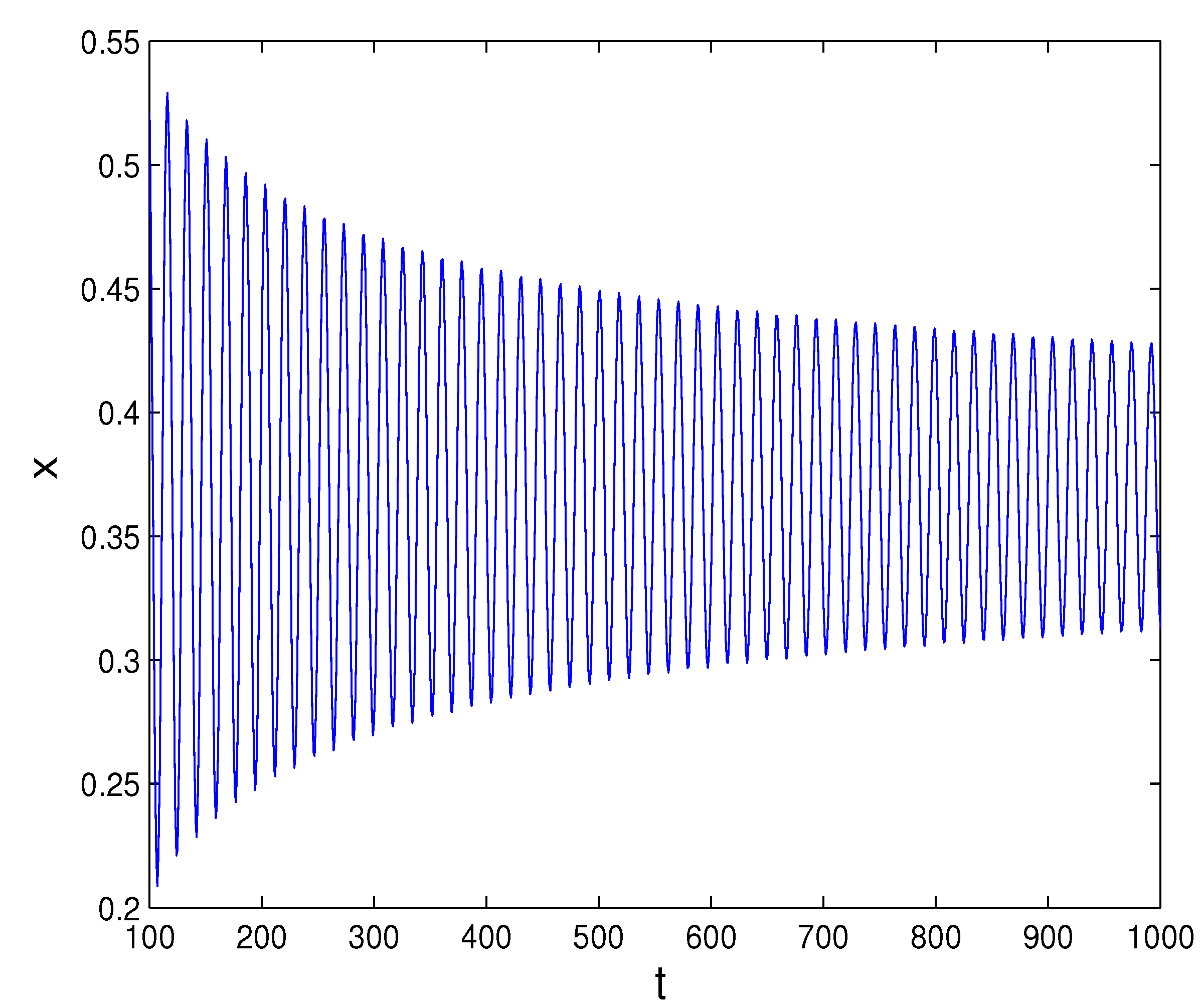
4.3. Numerical Example

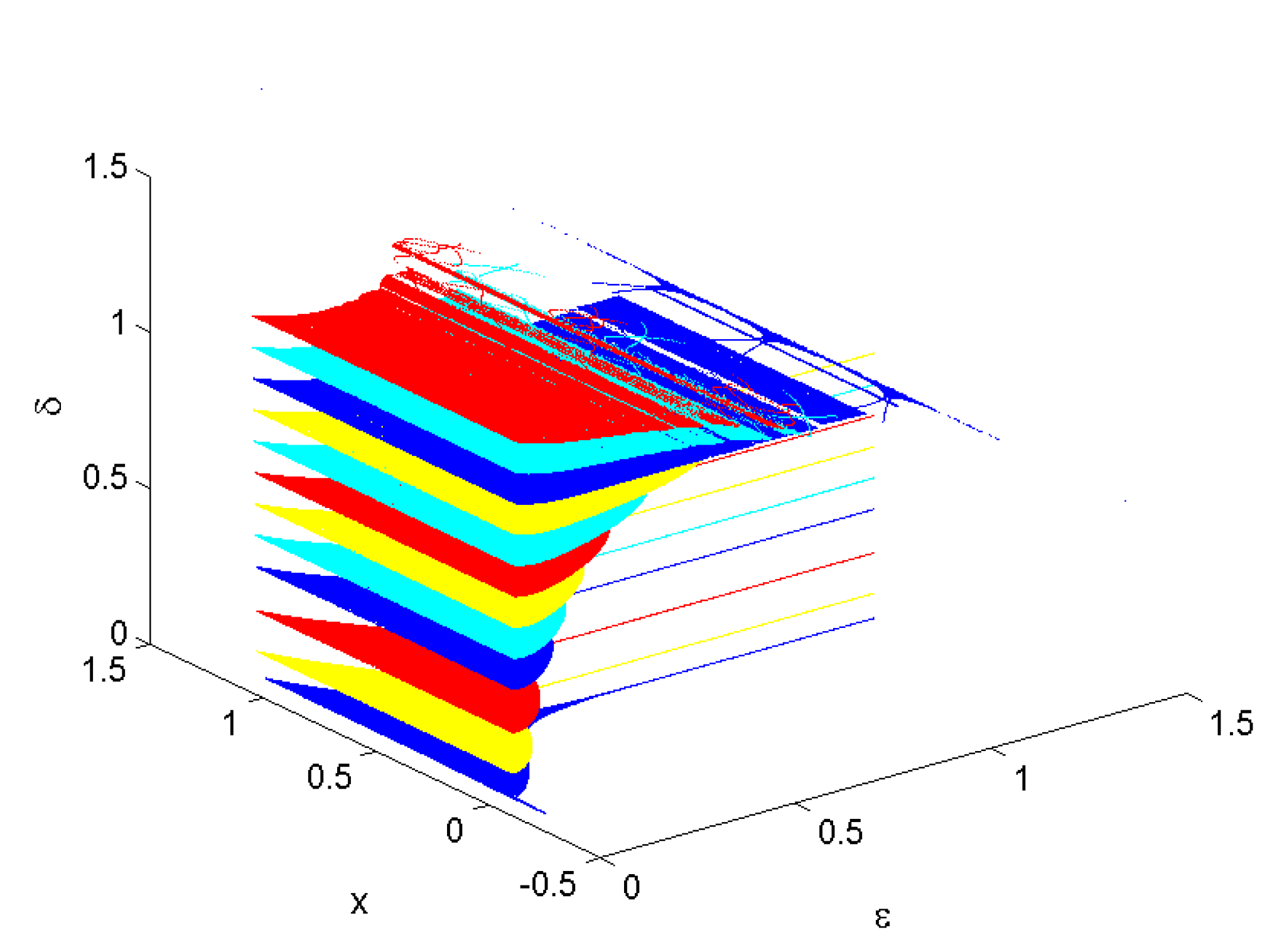
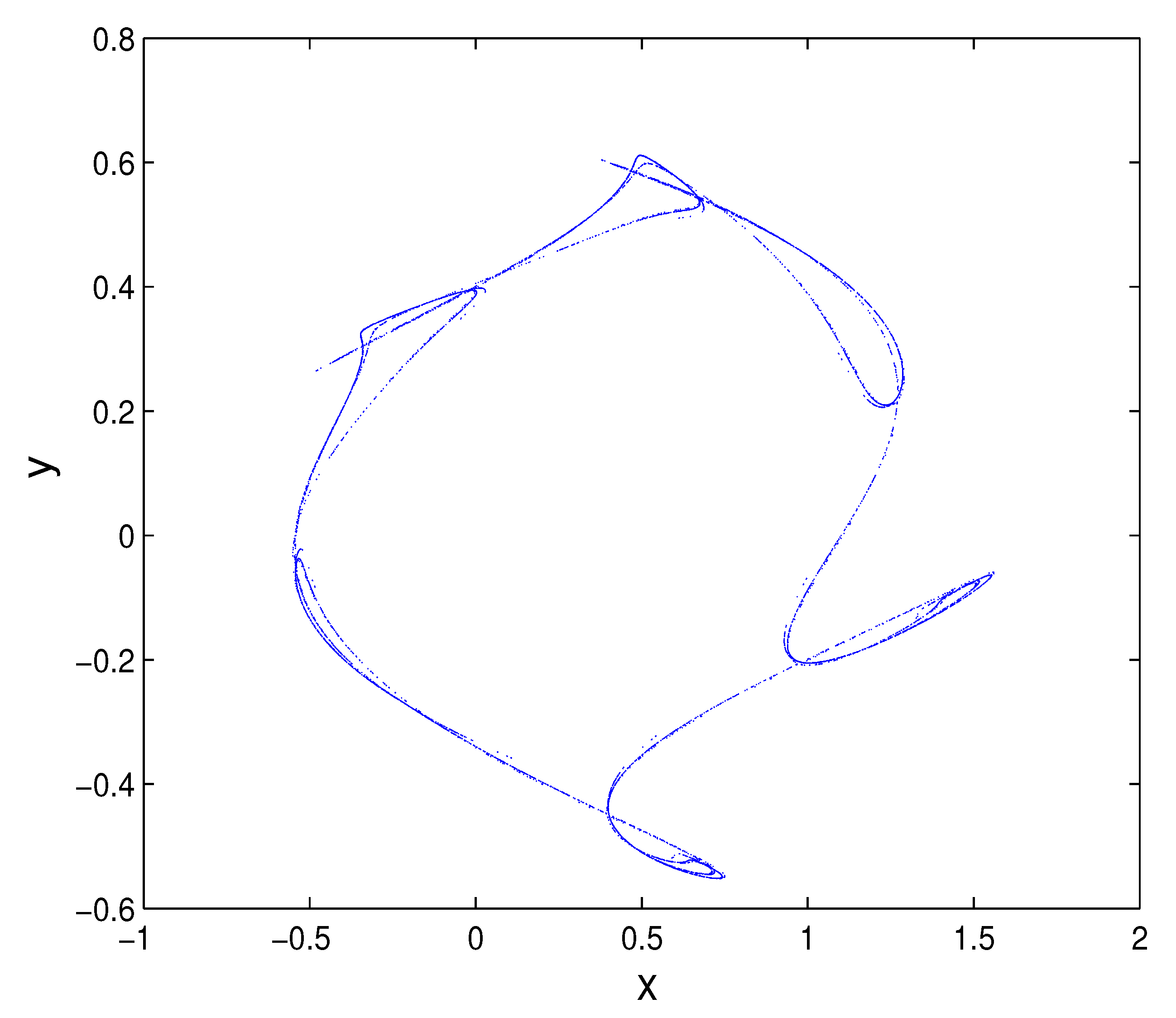
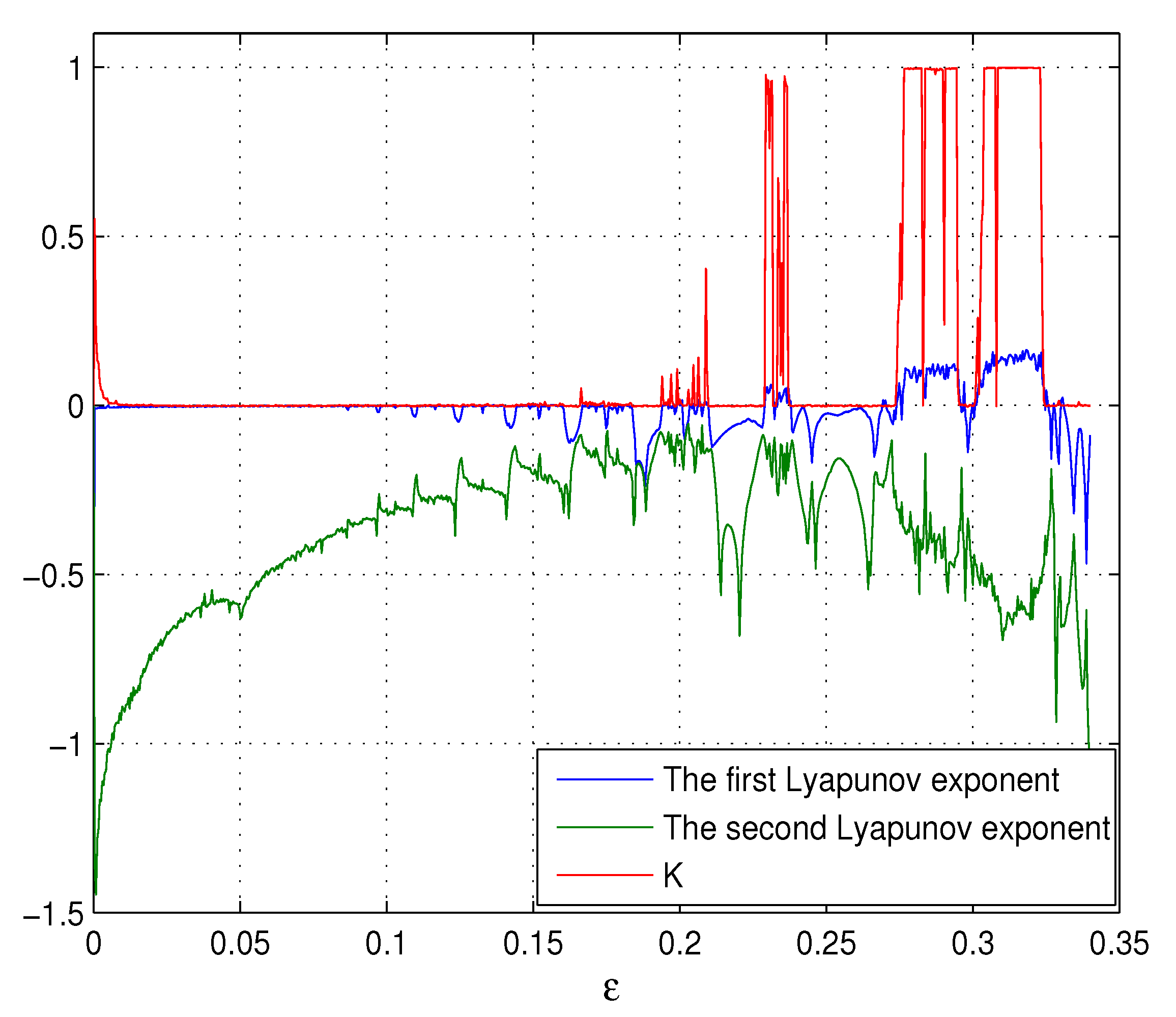
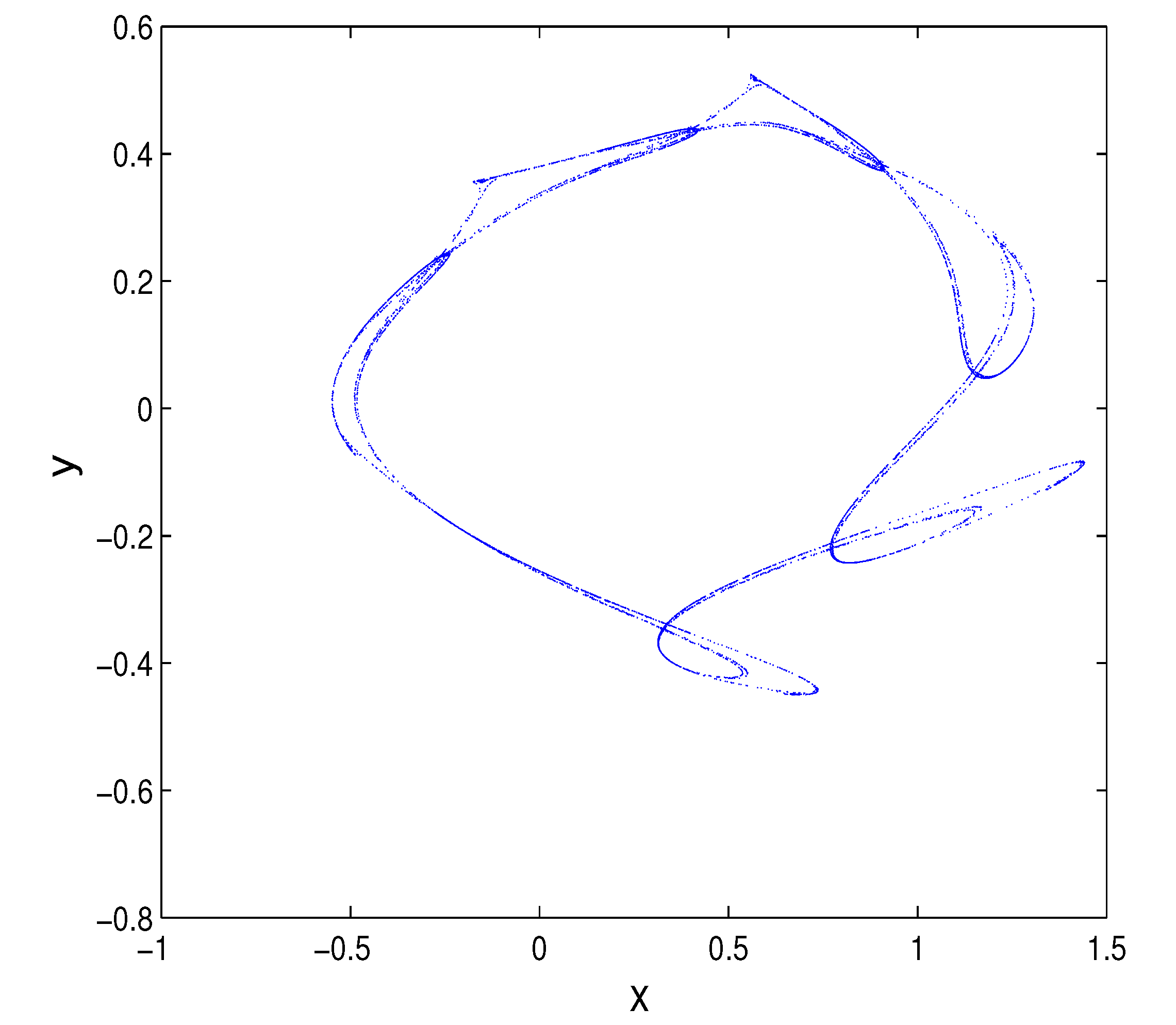
In this section, we will justify the above analytic results by means of a bifurcation diagram, phase portrait and evolution series diagram.

In what follows, we let $a=0.5,b=0.4$ and the initial state $(x_s,y_s)=(0.4,0.6)$; then, systemEquation (2) can be rewritten as the following form:

$$\left\{\begin{array}{cc}{x}_{n+1}\hfill & =x_n+\text{δ}(x_n(x_n-0.5)(1-x_n)-y_n)\hfill \\ y_{n+1}\hfill & =y_n+\text{ϵδ}(x_n-y_n-0.4)\hfill \end{array}\right.$$

(18)

which have a unique real-valued fixed point $E_0=(0.37,-0.03)$ and two complex conjugate fixed points $E_1=(0.57+i0.87,0.17+i0.87)$, $E_2=(0.57-i0.87,0.17-i0.87)$. The $E_1$ and $E_2$ are always complex conjugate and will not be considered here.

Figure 1 is the bifurcation diagram of x of the system Equation (18) with two parameters δ and ϵ. The bifurcation diagram illustrates the possible long-term values of the system Equation (18) as parameters δ and ϵ are varied. To produce Figure 1, ϵ varies from zero to 1.2 with an increment of 0.0024; and δ is sampled 12 values from zero to 1.2, and for x is used 300 data points after skipping 1000 transient data. Figure 1 can be regarded as a kind of superposition of bifurcation diagrams for 12 different values of δ. We plot Figure 1 to show bifurcation slices of xwith two parameters δ and ϵ. Each slice exhibits a bifurcation of x with the varying ϵ and a fixed δ. Figure 2 is the critical value curve of Neimark–Sacker bifurcation of system (18), which can be obtained from Equations (11) and (12). What is more, for combinations of parameters ϵ and δ in Figure 2, once crossing over the blue critical curve of Neimark–Sacker bifurcation and falling into the region on the left, the system Equation (18) must begin to undergo the Neimark–Sacker bifurcation. It is obvious that Figure 1 agrees well with Figure 2.

Figure 1. Bifurcation slices of x with parameters δ and ϵ.

Figure 2. The critical value curve of Neimark–Sacker bifurcation with parameters δ and ϵ.

The real-valued fixed point $E_0$ is shown in Figure 3, and the bifurcation diagram is shown inFigure 4. The above two figures indicate that the system Equation (18) is asymptotically stable with $\text{ϵ}=0.4$ and $\text{δ}<0.62773$.

According to Equations (11) and (12), one can take a critical bifurcation value pair $({\text{ϵ}}^{*},{\text{δ}}^{*})=(0.4,0.62733)$. Thus, there are $\left|{\lambda }_{\pm }\right|=1$ and $d(0.4,0.62733)=-6.676<0$. It follows from Proposition 2 and Figure 4 that a supercritical Neimark–Sacker bifurcation occurs at $({\text{ϵ}}^{*},{\text{δ}}^{*})=(0.4,0.62733)$ of system Equation (18).

When one gives a small perturbation $▵\text{δ}=0.001$, a sufficiently small real number, i.e., $\text{δ}={\text{δ}}^{*}+▵\text{δ}=0.62733+0.0001=0.62833$, the system Equation (18) has a stable, closed invariant curve around the the fixed point (quasi-periodic solution), as shown in Figure 5. Furthermore, Figure 6 represents that the solution in the system Equation (18) asymptotically approaches a unique invariant closed circle, i.e., the Neimark–Sacker bifurcation is supercritical.

Figure 3. Phase portrait with ϵ =0.4 and δ =0.5.

Figure 4. Bifurcation diagram for System (18) with ϵ =0.4.

Figure 5. Phase portrait with ϵ =0.4 and δ =0.62833.

Figure 6. Evolution series of x with ϵ =0.4 and δ =0.62833.

5. Chaos

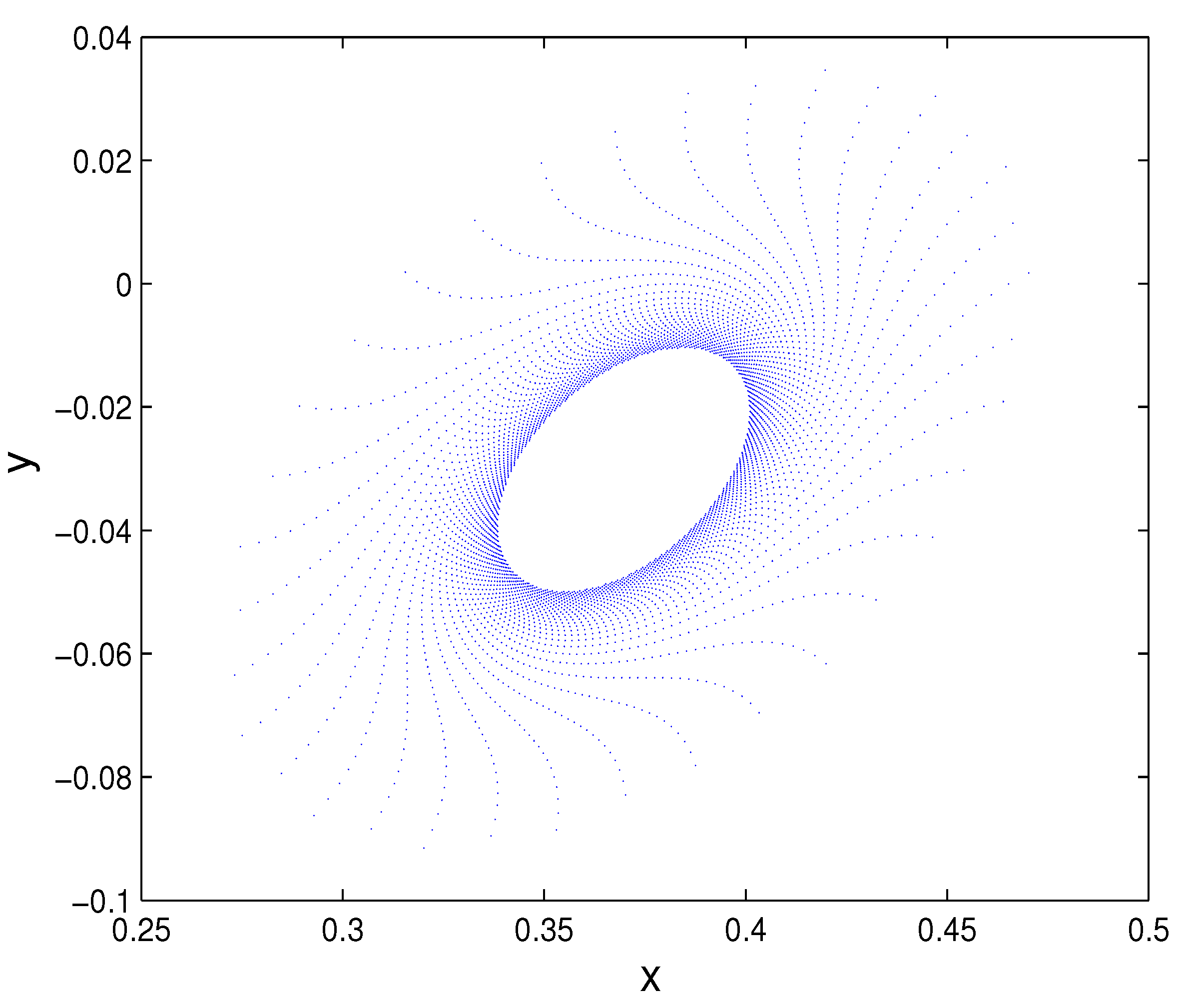
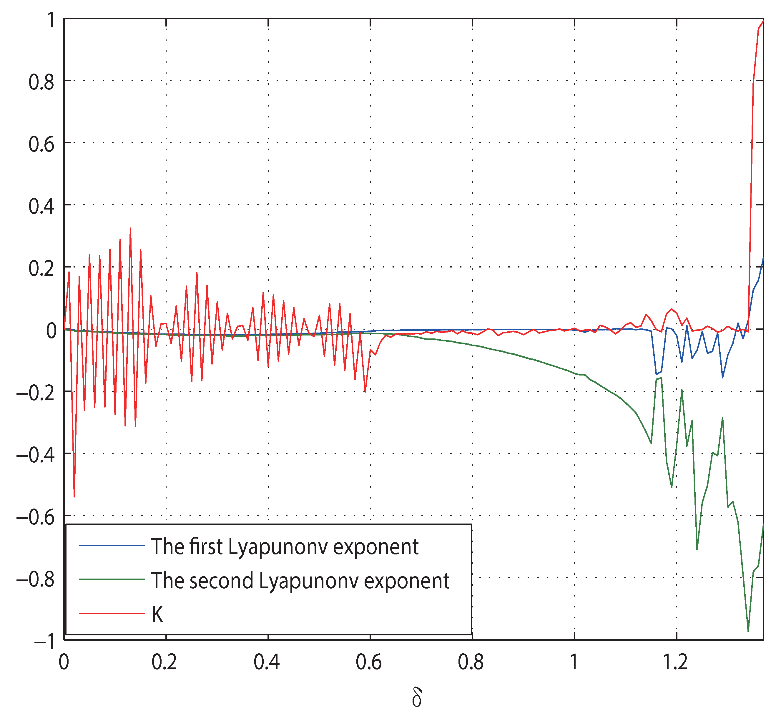
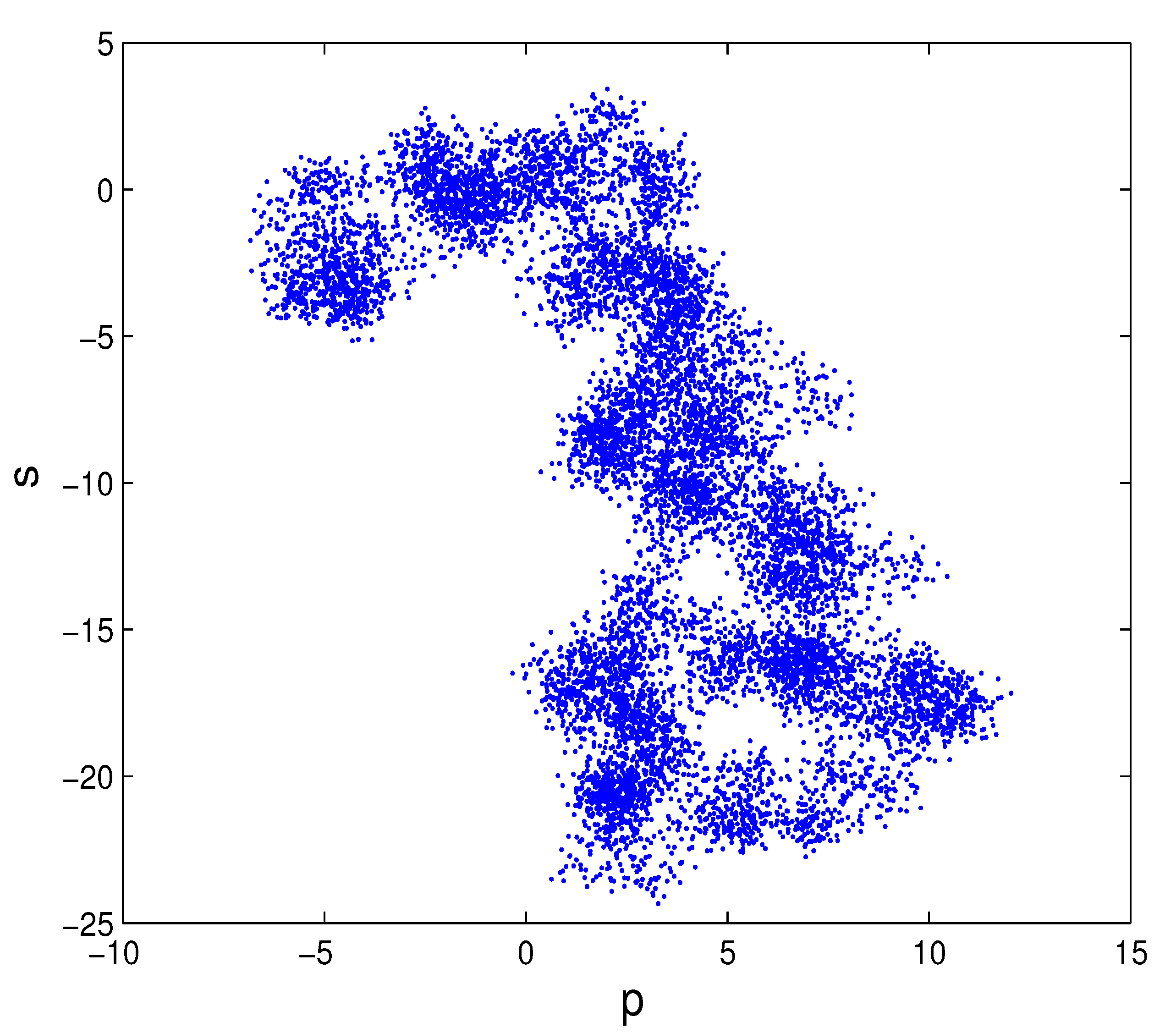
5.1. 0–1 Test Algorithm for Chaos

We can formulate the 0–1 test algorithm [16,17,18,19,20,21] as follows.

Suppose ϕ$\left(n\right)$ is a discrete set of measurement data sampled at times $n=1,2,3,\cdots ,N$, where N is the total amount of the data.

Step 1: Choose a random number $cϵ(\frac{\pi }{5},\frac{4\pi }{5})$, then define the new coordinates $\left(p_c\left(n\right),s_c\left(n\right)\right)$ as follows.

$$\begin{array}{c}\hfill p_c\left(n\right)=\sum _{j=1}^n\text{ϕ}\left(j\right)cos\left(\text{θ}\left(j\right)\right)\\ \hfill s_c\left(n\right)=\sum _{j=1}^n\text{ϕ}\left(j\right)sin\left(\text{θ}\left(j\right)\right)\end{array}$$

(19)

where:

$$\begin{array}{c}\hfill \text{θ}\left(j\right)=jc+\sum _{i=1}^j\text{ϕ}\left(j\right),j=1,2,3,\cdots ,n\end{array}$$

Step 2: Define the mean square displacement $M_c\left(n\right)$ as follows:

$$\begin{array}{c}\hfill M_c\left(n\right)=\underset{N\to \infty }{lim}\frac{1}{N}\sum _{j=1}^N{\left(p_c(j+n)-p_c\left(j\right)\right)}^2+{\left(s_c(j+n)-s_c\left(j\right)\right)}^2,nϵ[1,\frac{N}{10}]\end{array}$$

(20)

Step 3: Define the modified mean square displacement $D_c\left(n\right)$ as follows:

$$\begin{array}{c}\hfill D_c\left(n\right)=M_c\left(n\right)-{\left(\underset{N\to \infty }{lim}\frac{1}{N}\sum _{j=1}^N\text{ϕ}\left(j\right)\right)}^2\frac{1-cosnc}{1-cosc}\end{array}$$

(21)

Step 4: Define the median value of correlation coefficient K as follows:

$$\begin{array}{c}\hfill K=median\left(K_c\right)\end{array}$$

(22)

where:

$$\begin{array}{c}\hfill K_c=\frac{cov(\xi ,\text{Δ})}{\sqrt{var\left(\xi \right)var\left(\text{Δ}\right)}}ϵ[-1,1]\end{array}$$

in which $\xi =(1,2,3,\cdots ,n_{cut}),\text{Δ}=(D_c\left(1\right),D_c\left(2\right),\cdots ,D_c\left(n_{cut}\right)),n_{cut}=round\left(\frac{N}{10}\right)$, and the covariance and variance are defined with vectors $x,y$ of length q as follows:

$$\begin{array}{c}cov(x,y)=\frac{1}{q}\sum _{j=1}^q\left(x\left(j\right)-\overline{x}\right)\left(y\left(j\right)-\overline{y}\right)\hfill \\ \overline{x}=\frac{1}{q}\sum _{j=1}^{q}x\left(j\right)\hfill \\ var\left(x\right)=cov(x,x)\hfill \end{array}$$

Step 5: Interpret the outputs as follows:

(1) $K\approx 0$ indicates that the underlying dynamics is regular (i.e., periodic or quasi-periodic), whereas $K\approx 1$ indicates that the underlying dynamics is chaotic.

(2) Bounded trajectories in the $(p,s)$-plane imply that the underlying dynamics is regular, whereas for Brownian-like (unbounded) trajectories, the underlying dynamics is chaotic.

In periodic dynamics, there are isolated values of c for which $K_c$ is large due to resonances, so it is suggested to use the median of the computed values of $K_c$ as $K=median\left(K_c\right)$. In practice, 100 choices of c is sufficient to get various values $K_c$ versus c [21,22]. In this work, we let $N=9500$ and use 100 random c values in $[\pi /5,4\pi /5]$.

5.2. Numerical Example

We sample the dataset x from system Equation (18) and let the time series length $N=9500$, parameters $\text{ϵ}\in [0,0.34]$ and $\text{δ}\in [0,1.37]$, initial values $x_1=0.4$ and $y_1=0.6$. The 0–1 test with ϵ and δ will be implemented as follows, respectively.

As mentioned in Subsection 3.2 and shown in Figure 2, if $\text{ϵ}=0.4$ is fixed, the point $(\text{ϵ},\text{δ})=(0.4,0.6273)$ is the critical point of the Neimark–Sacker bifurcation of system Equation (18). Therefore, the region with $\text{δ}\in [0,0.6273)$ is stable, and the other region with $\text{δ}\in (0.6273,1.37]$ is unstable, where chaos may occur. With δ varying from zero to $1.37$ in increments of $0.001$, one can get the diagram of the K value and Lyapunov exponents shown in Figure 7. There is a very good agreement between Figure 7 and the bifurcation diagram shown in Figure 4. From Figure 4 and Figure 7, one can find that chaos occurs when $\text{δ}\in [1.35,1.37]$, where $K\approx 1$, which means that the system has chaotic movement. When $\text{δ}=1.36$, Figure 8 presents a chaotic attractor in the original state space $(x,y)$, and Figure 9 denotes the plots with the transformed coordinates $(p,s)$, where Brownian-like trajectories denote that the system Equation (18) is chaotic.

Figure 7. Lyapunov exponents and K versus δ for system Equation (18) with ϵ =0.4.

Figure 8. Plot of in the original state space (x,y) for system Equation (18) with ϵ =0.4 and δ =1.36.

Figure 9. Plot in the new coordinates (p,s) space for system Equation (18) with ϵ = 0.4 and δ = 1.36.

As shown in Figure 2, if $\text{δ}=1.44$ is fixed, then points $(\text{ϵ},\text{δ})$ must locate above the critical value curve of the Neimark–Sacker bifurcation of system Equation (18) for arbitrary $\text{ϵ}\in [0,1.5]$. With ϵ varying from zero to $0.34$ in increments of $0.000425$, one can get the diagram of the K value and Lyapunov exponents shown in Figure 10, which is consistent with the bifurcation diagram shown in Figure 11. From Figure 10 and Figure 11, one can find that chaos occurs when $\text{ϵ}\in [0.229,0.237]\bigcup [0.279,0.294]\bigcup [0.306,0.321]$, where $K\approx 1$, which means that the system is chaotic. Let $\text{ϵ}=0.32$; Figure 12 presents a strange attractor in the original state space $(x,y)$, and Figure 13 shows the plot with the transformed coordinates $(p,s)$, where Brownian-like trajectories indicate that the dynamics of system Equation (18) is undergoing chaos.

Figure 10. Lyapunov exponents and K versus ϵ for system Equation (18) with δ =1.44.

Figure 11. Bifurcation diagram versus ϵ in the original state space for system Equation (18) with δ =1.44.

Figure 12. Plot of in the original state space (x,y) for system Equation (18) with δ =1.44 and ϵ =0.32.

Figure 13. Plot in the new coordinates (p,s) space for system Equation (18) with δ =1.44 and ϵ =0.32.

6. Conclusions

(i) We proposed a discrete complex interaction model about industrial production and environmental quality in a closed area, which can help us understand the above dynamical interaction mechanism from the environmental sustainability perspective.

(ii) We calculated the critical value, direction and stability of Neimark–Sacker bifurcation of the discrete-time interaction model, which can help us make use of its attribution of the Neimark–Sacker bifurcation of the interaction system and even control it.

(iii) We employed the 0–1 test algorithm to verify the chaos of the model, which can help us find and utilize the chaos of the interaction system and even control it.

References

- Salomone, R.; Clasadonte, M.; Proto, M.; Raggi, A. (Eds.) Product-oriented environmental management system (POEMS): A sustainable management framework for the food industry. Available online http://www.lcm2011.org/papers.html?file=tl_files/pdf/poster/day1/Salomone-Product-Oriented_Environmental_Management_System-651_b.pdf (accesseed on 24 July 2015).
- Salomone, R.; Ioppolo, G.; Saija, G. Product-Oriented Environmental Management Systems (POEMS); Springer: Dordrecht, The Netherlands, 2013; pp. 257–302. [Google Scholar]
- Salomone, R.; Ioppolo, G. Environmental impacts of olive oil production: A Life Cycle Assessment case study in the province of Messina (Sicily). J. Clean Prod. 2012, 28, 88–100. [Google Scholar] [CrossRef]
- Zhao, N.; Liu, Y.; Chen, J. Regional industrial production's spatial distribution and water pollution control: A plant-level aggregation method for the case of a small region in China. Sci. Total Environ. 2009, 407, 4946–4953. [Google Scholar] [CrossRef] [PubMed]
- Aşıcı, A. Economic growth and its impact on environment: A panel data analysis. Ecological. Indic. 2013, 24, 324–333. [Google Scholar] [CrossRef]
- Dinda, S. Environmental Kuznets curve hypothesis: A survey. Ecol. Econ. 2004, 49, 431–455. [Google Scholar] [CrossRef]
- Copeland, B.; Taylor, M. Trade, growth, and the environment. J. Econ. Literat. 2004, 42, 7–71. [Google Scholar] [CrossRef]
- Paraschiv, D.; Tudor, C.; Petrariu, R. The Textile Industry and Sustainable Development: A Holt-Winters Forecasting Investigation for the Eastern European Area. Sustainability 2015, 7, 1280–1291. [Google Scholar] [CrossRef]
- Aliehyaei, M.; Atabi, F.; Khorshidvand, M.; Rosen, M. Exergy, Economic and Environmental Analysis for Simple and Combined Heat and Power IC Engines. Sustainability 2015, 7, 4411–4424. [Google Scholar]
- Kuznetsov, J. Elements of Applied Bifurcation Theory; Springer: New York, NY, USA, 1998. [Google Scholar]
- Wen, G.; Xu, D.; Han, X. On creation of Hopf bifurcations in discrete-time nonlinear systems. Chaos 2002, 12, 350–355. [Google Scholar] [CrossRef] [PubMed]
- Wen, G. Criterion to identify Hopf bifurcations in maps of arbitrary dimension. Phys. Rev. E 2005, 72, 26201. [Google Scholar] [CrossRef]
- Xin, B.; Chen, T.; Ma, J. Neimark–Sacker Bifurcation in a Discrete-Time Financial System. Discrete Dynam. Nat. Soc. 2010, 2010, 405639. [Google Scholar] [CrossRef]
- Xin, B.; Ma, J.; Gao, Q. The complexity of an investment competition dynamical model with imperfect information in a security market. Chaos Soliton. Fract. 2009, 42, 2425–2438. [Google Scholar] [CrossRef]
- Li, E.; Li, G.; Wen, G.; Wang, H. Hopf bifurcation of the third-order He´non system based on an explicit criterion. Nonlinear Anal Theor. Meth. Appl. 2009, 70, 3227–3235. [Google Scholar] [CrossRef]
- Gottwald, G.; Melbourne, I. A new test for chaos in deterministic systems. Proc. R. Soc. Lond. Ser. A 2004, 460, 603–611. [Google Scholar] [CrossRef]
- Xin, B.; Li, Y. 0–1 test for chaos in a fractional order financial system with investment incentive. Abstr. Appl. Anal. 2013, 2013, 876298. [Google Scholar] [CrossRef]
- Xin, B.; Li, Y. Bifurcation and Chaos in a Price Game of Irrigation Water in a Coastal Irrigation District. Discrete Dynam. Nat. Soc. 2013, 2013, 408904. [Google Scholar] [CrossRef]
- Xin, B.; Wu, Z. Projective Synchronization of Chaotic Discrete Dynamical Systems via Linear State Error Feedback Control. Entropy 2015, 17, 2677–2687. [Google Scholar] [CrossRef]
- Gottwald, G.; Melbourne, I. On the Implementation of the 0–1 Test for Chaos. SIAM J. Appl. Dynam. Syst. 2009, 8, 129–145. [Google Scholar] [CrossRef]
- Falconer, I.; Gottwald, G.; Melbourne, I.; Wormnes, K. Application of the 0-1 test for chaos to experimental data. SIAM J. Appl. Dynam. Syst. 2007, 6, 395–402. [Google Scholar] [CrossRef]
- Gottwald, G.; Melbourne, I. On the validity of the 0–1 test for chaos. Nonlinearity 2009, 22, 1367–1382. [Google Scholar] [CrossRef]
- Litak, G.; Syta, A.; Wiercigroch, M. Identification of chaos in a cutting process by the 0–1 test. Chaos Soliton. Fract. 2009, 40, 2095–2101. [Google Scholar] [CrossRef]
- Bizjan, B.; Sirok, B.; Govekar, E. Nonlinear Analysis of Mineral Wool Fiberization Process. J. Comput. Nonlinear Dynam. 2015, 10, 021005. [Google Scholar] [CrossRef]
- Krese, B.; Govekar, E. Nonlinear analysis of laser droplet generation by means of 0–1 test for chaos. Nonlinear Dynam. 2012, 67, 2101–2109. [Google Scholar] [CrossRef]
© 2015 by the authors; licensee MDPI, Basel, Switzerland. This article is an open access article distributed under the terms and conditions of the Creative Commons Attribution license (http://creativecommons.org/licenses/by/4.0/).