Abstract
This study investigates the effects of compact urban development on air pollution, taking into account both the spatial distribution of pollutants resulting from an increase in inner urban densities and the dispersion of pollutants associated with an increase in outer green open spaces. The empirical analysis is based upon a panel data model covering 17 cities in Korea from 1996–2009; this approach is used because urban air pollution is influenced by spatial and temporal changes. Measuring the air pollution level by distance from city centers demonstrates that the spatial concentration of emission sources does not necessarily increase air pollution levels. The two-way fixed effects model, which is employed to control both individual (regional) and time effects, shows that SO2 decreases as the proportion of green area increases, while a rise in net density leads to an increase of NO2. Both effects are observed in the case of CO dispersion by green area as well as emission source concentration by high densities. Therefore, there is no clear impact of compact urban development on air quality, which is instead related to pollutant-specific characteristics and the emission source.
1. Introduction
Urban growth has caused many environmental problems, especially urban sprawl which leads to loss of green open spaces and an increase in traffic and energy consumption. As a result, the compact city concept has been put forward as a form of sustainable urban development. Air pollution is one of the key environmental problems associated with urbanization. This has brought researchers to question whether or not compact cities contribute to air pollution reduction.
Compact urban development would likely have both positive and negative effects on air quality. Supporters of the compact city concept assert that high-density development can result in reduced car dependency, reduced energy consumption, and low emissions via a decrease in distance traveled [1,2,3,4,5,6,7]. Specifically, it has been demonstrated that large metropolitan regions ranking highly on a quantitative index of sprawl experience a greater number of O3 exceedances in comparison to more spatially compact metropolitan regions [6]. The significant association of nitrogen oxides (NOx) and volatile organic compounds (VOCs) suggests that urban spatial structure plays a role in O3 formation through its effects on O3 precursor emissions from transportation, industry, and power generation facilities. Vehicle emissions of CO and NOx have been found to exhibit a significant negative relationship with household and employment density [3].
Opponents of high-density developments contend that, as they concentrate many activities in a limited space, they usually cause increased air pollution [8]. Higher densities lead to traffic congestion and greater air pollution [9,10,11]. Large cities pollute more and generate more environmental damage than medium-sized ones; for example, higher levels of production, linked to increasing physical urban size, likely resulted in higher pollution densities in Italian cities [12].
The relationship between reductions in pollution levels and spatial concentration of emission sources by compact urban development has been investigated, with researchers reaching the conclusion that the negative effects were relatively larger than the positive effects [13]. That is, an increase in air pollution resulted from the spatial concentration of emission sources and this was shown to be greater than the amount of reduction in pollution levels caused by a decrease in transportation-related energy. Meanwhile, there are also claims that compactness has no statistical relationship with air pollution [14].
Despite the different arguments, the existing literature has still overlooked one important natural phenomenon that influences air pollution. Emitted air pollutants disperse and dilute in the atmosphere [15] and move freely according to the flow of air. Atmospheric dispersion and dilution of air pollutants are strongly influenced by meteorological conditions and topographical features, and urban structures have a great effect on meteorological parameters such as wind direction, wind speed, turbulence, and atmospheric stability [16]. The dispersion and dilution processes result in ambient air pollution, which shows concentrations of different substances varying in relation to time and space [16].
Accordingly, urban air pollution is affected by the dispersion and dilution processes and is characterized by the spatial variability of pollutants [9,17]. The transport and dispersion of pollutants over an urban area is altered as a result of increased mechanical turbulence caused by the relatively large obstacles (i.e., buildings and other structures) over which pollutants must travel [18]. Greater topographic unevenness of the terrain produces a significant increase in turbulence levels, which leads to greater dilution of a pollutant plume and reduced concentrations downwind [19,20]. In Korea, in a study considering the pollutant transmission and dispersion processes, the maximum concentration of particles was shown as being between 50 and 60 km from the source [21]. The gaseous pollutants’ concentrations were lower at the location closest to the heat source rather than farthest from the source [22].
Furthermore, it has been reported that the dispersion and dilution of air pollutants is related to open green spaces. Open spaces planted with trees, shrubs, and grasses alter the local climate, increasing wind speeds and reducing temperatures, thereby encouraging air circulation and thus increasing the dispersion of pollutants [23]. Vegetation also directly absorbs pollutants through its foliage, thus reducing air pollution levels [24]. The average concentration of pollutants (particularly particulates) declines with increasing proportions of planted open spaces [25]. Even very small areas of open space in an urban area can reduce particulate pollution levels [26].
Some studies have revealed the link between urban design issues, such as compactness or sprawl and air quality, namely atmospheric dispersion and dilution through simulations [1,27,28,29]. Nonetheless, researchers—arguing both for and against compact city structure—are still hampered by the absence of empirical evidence to support the effects of increased urbanization on air pollution. This study attempts to draw attention to something that the existing literature has not covered for the most part, underlining that air pollution problems from urban development are mid to long term and cumulative [30], and that air pollution concentrations are determined by dispersion and dilution processes that vary in relation to time and space. We ask whether or not compact cities contribute to air pollution reduction, considering that air pollution is influenced by spatial and temporal changes in urban characteristics as well as by dispersion and dilution processes in the atmosphere. If more green areas are secured in the surroundings of a city through compact development, this will increase the dispersion and dilution of pollutants, which can, in turn, result in lower air pollution levels. In this regard, this study attempts to investigate the effects of compact urban development on air pollution taking into account both the spatial concentration of pollutant sources resulting from an increase in inner urban density and the dispersion of pollutants associated with an increase in outer green open spaces. The empirical analysis is conducted on data from 1996–2009 obtained from automatic air quality monitoring stations located in 17 Korean cities, focusing on five major pollutants: SO2, NO2, CO, O3, and PM10.
2. Spatial Distribution Pattern of Air Pollution
2.1. Data and Methods
If only the spatial concentration of pollutant sources were a major contributor to urban air pollution, air pollution levels would be highest at the city center [33] and decrease with distance. However, if dispersion due to convection currents occurs, air pollution levels will not necessarily get higher with closer proximity to the city center. Therefore, there is a need to verify this empirically. We used a least squares linear regression for each pollutant to determine if a relationship existed between air pollution levels and distance from the city centers. Air pollution level (the dependent variable) was regressed on distance from city centers (the independent variable) in order to verify whether the estimated slope coefficients were statistically significant with negative interactions.
Air quality data for five classical major pollutants (i.e., SO2, NO2, CO, O3, and PM10) were obtained for the period 1996–2009 from the Annual Report on Ambient Air Quality (1997–2010) in Korea [34,35]. Gas-phase pollutant levels, collected from 17 cities [36] with populations in excess of 200,000 people, were used in our study as determined by the availability and consistency of measured data. PM10 data was obtained for nine cities [37] dependent on data availability. Air pollutant concentrations are expressed as annual average concentrations except for ozone, which is expressed as the annual average of the maximum daily eight-hour measurement period. The city centers of the 17 individual cities were identified and the distance from city center to the air quality monitoring stations was calculated through GIS (ArcGIS 10.0). Measuring the distance was used on the function of “measure a line” among the GIS’s tools on the basis of a digital topographic map with a scale of 1:25,000 [38]. The range of distance was from 0–23.45 km. There are varying numbers of air quality monitoring stations in each city, with numbers gradually increasing on an annual basis [39].
2.2. Air Pollution Level by Distance from City Center
The air pollution levels of the five pollutants were scattered by distance from the city centers (Figure 1, Figure 2, Figure 3, Figure 4 and Figure 5). There was no clear pattern suggesting that sites closer to the city centers had higher air pollution levels [40]. For presentation convenience, regressions are aggregated by year and the regression lines for each year are shown in Figure 1, Figure 2, Figure 3, Figure 4 and Figure 5. The estimated slope coefficients are presented in Table 1.
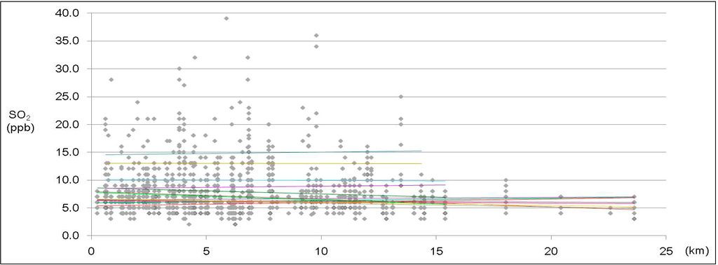
Figure 1.
Distribution of SO2 annual averages by distance from city centers and regression lines for each year (1996–2009).
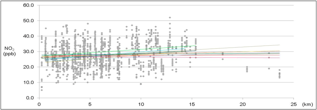
Figure 2.
Distribution of NO2 annual averages by distance from city centers and regression lines for each year (1996–2009).
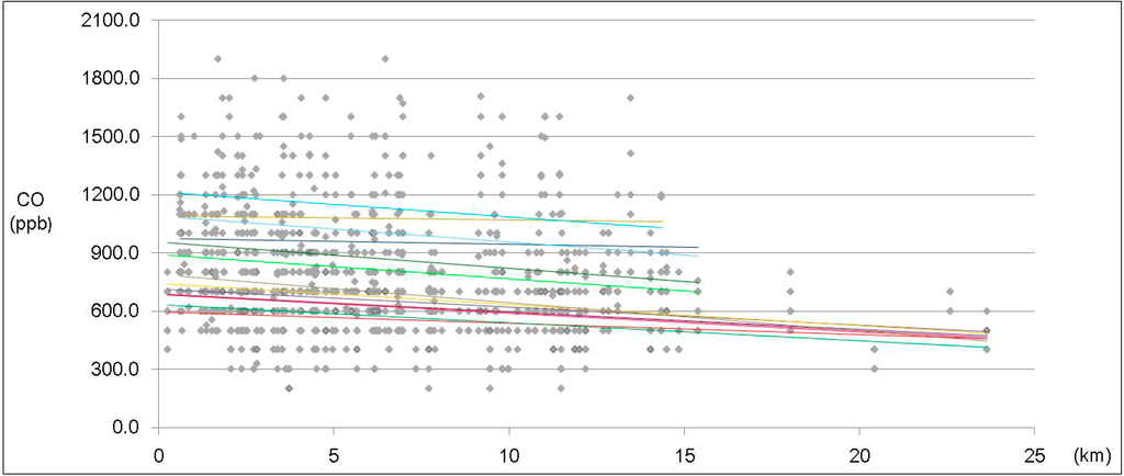
Figure 3.
Distribution of CO annual averages by distance from city centers and regression lines for each year (1996–2009).
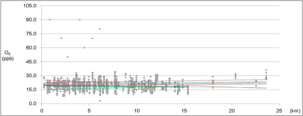
Figure 4.
Distribution of 8-h daily max O3 annual averages by distance from city centers and regression lines for each year (1996–2009).
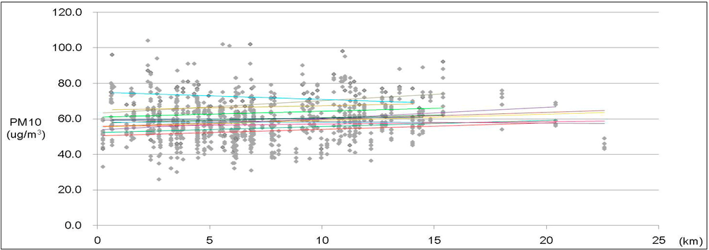
Figure 5.
Distribution of PM10 annual averages by distance from city centers and regression lines for each year (1996–2009).

Table 1.
Estimated slope coefficients for five pollutants (1996–2009).
| SO2 (ppb) | NO2 (ppb) | CO (ppb) | O3 (ppb) | PM10 (µg/m3) | |
|---|---|---|---|---|---|
| 1996 (R2) | 0.052 (8.28 × 10⁻⁴) | 0.506 * (0.06) | −12.718 (0.02) | 0.238 (0.03) | −0.410 (1.20 × 10⁻²) |
| 1997 (R2) | −0.006 (1.75 × 10⁻⁵) | 0.498 * (0.05) | −2.032 (6.74 × 10⁻⁴) | 0.186 (0.02) | 0.240 (4.46 × 10⁻³) |
| 1998 (R2) | −0.016 (2.14 × 10⁻⁴) | 0.284 (0.03) | −13.397 (0.04) | 0.004 (1.21 × 10⁻⁵) | 0.001 (6.00 × 10⁻⁸) |
| 1999 (R2) | 0.041 (2.35 × 10⁻⁵) | 0.374 (0.04) | −2.967 (1.78 × 10⁻³) | −0.070 (5.16 × 10⁻³) | 0.109 (1.14 × 10⁻³) |
| 2000 (R2) | −0.111 (0.02) | 0.323 (0.02) | −13.592 (0.04) | −0.058 (3.10 × 10⁻³) | 0.286 (8.38 × 10⁻³) |
| 2001 (R2) | −0.137 (0.03) | 0.446 * (0.06) | −12.530 (0.03) | −0.141 (0.01) | 0.333 (9.90 × 10⁻³) |
| 2002 (R2) | −0.070 (0.02) | 0.371 (0.04) | −14.693 ** (0.11) | −0.102 (7.17 × 10⁻³) | 0.707 (0.04) |
| 2003 (R2) | −0.057 (9.80 × 10⁻³) | 0.158 (6.12 × 10⁻³) | −10.954 ** (0.08) | −0.091 (7.26 × 10⁻³) | 0.361 (0.01) |
| 2004 (R2) | −0.018 (1.15 × 10⁻³) | 0.077 (2.11 × 10⁻³) | −10.020 ** (0.07) | 0.055 (2.70 × 10⁻³) | −0.084 (1.66 × 10⁻³) |
| 2005 (R2) | −0.021 (2.39 × 10⁻³) | −0.035 (5.62 × 10⁻³) | −9.716 ** (0.06) | 0.060 (5.35 × 10⁻³) | 0.131 (3.49 × 10⁻³) |
| 2006 (R2) | −0.138 (0.02) | 0.095 (3.12 × 10⁻³) | −8.810 ** (0.06) | −0.380 (0.01) | 0.401 * (0.04) |
| 2007 (R2) | 0.022 (2.50 × 10⁻³) | 0.128 (4.55 × 10⁻³) | −9.062 ** (0.06) | 0.101 (0.01) | 0.639 ** (0.12) |
| 2008 (R2) | 0.041 (8.08 × 10⁻³) | 0.037 (3.89 × 10⁻⁴) | −9.411 ** (0.07) | 0.076 (7.02 × 10⁻³) | 0.341 * (0.05) |
| 2009 (R2) | 0.060 (0.02) | 0.011 (4.11 × 10⁻⁵) | −5.881 * (0.04) | 0.133 (0.02) | 0.358 (0.04) |
* p < 0.5; ** p < 0.01.
The estimated slope coefficients are not always negative, implying that air pollution levels do not necessarily decrease as the distance from the city center increases. Moreover, most of them are not statistically significant, and thereby we cannot reject the null hypothesis (i.e., that the slope is 0), implying that air pollution levels do not vary depending on distance from the city center. Only some of the pollutants are statistically significant and were negative (i.e., 2002 through 2009 for CO), but there were also other cases in which the coefficients are statistically significant and positive (1996, 1997, and 2001 for NO2 and 2006 through 2008 for PM10), meaning that air pollution levels increased with distance. Therefore, the results are inconsistent and it was difficult to make the generalization that the spatial concentration of pollutant sources resulted from compact urban development and increased air pollution levels near city centers.
3. Urban Compactness and Air Pollution
3.1. Data and Model
To further investigate the effects of compact urban development on air pollution, multi-dimensional panel data models were employed. The panel data model [41] is a quantitative analytical method that can be used when time-series and cross-section data are both available. Air pollution in cities is influenced by spatial characteristics (e.g., locational characteristics such as coastal or inland, geological characteristics such as mountains or plains, etc.) and periodic characteristics (e.g., changes in climatic conditions) and, therefore, spatial and temporal variations need to be taken into consideration at the same time in a panel analysis.
The panel data model handles variables that are important to the model but that are not included as explanatory variables. Another advantage is that it can also regulate estimate errors that arise from time-series processes and regional unit data. The model helps overcome the limitations of insufficient sample size (i.e., data) which were a cross-section of 17 cities and 14 year time series in this study. Considering that the atmospheric dispersion can be dependent on the location of city (e.g., whether cities are located inland or close to the coast), the location of city is an important factor. However, it was not used as an independent variable as city location does not change over time. For these reasons, the panel data model is an ideal analytical method for this study, considering that it can account for an unobservable omitted variable that has a significant effect on interurban air pollutant concentration differences.
To regulate omitted variables, error terms are categorized as variables such as individual (regional)-variant but time-invariant (or time-constant) or time-variant but individual-invariant. It also includes remainder stochastic disturbance term that is both dependent on individual and time.
The estimation equation for the panel data model is given below [42]:
- Yit = α + Xitβ + εit
- where εi,t = μi + λt + νi,tεi,t = μi + λt + νi,t, i (region) = 1, 2, ..., N, t (year) = 1, 2, ..., T
- μi = unobservable individual effect
- λt = unobservable time effect
- νi,t = remainder stochastic disturbance term.
The model is divided into either a fixed effects model (FEM) or a random effects model (REM) depending on the form of the error term. In the FEM, it is assumed that each subject has its own specific characteristics due to inherent individual characteristic effects in the error term, thereby allowing differences to be intercepted between subjects. Fixed effects are due to the fact that, although the intercept may differ across subjects, each entity’s intercept does not vary over time—that is, it is time-invariant [43]. The REM assumes that the individual characteristic effect changes stochastically, and that differences in subjects are not fixed in time and are independent between subjects. Individual differences vary over cross-sections (i.e., subjects) as well as time [44].
Air pollution levels, as dependent variables, were obtained by averaging observed measurements from each monitoring station in each of the 17 cities (nine in the case of PM10). There was little concern about using the averaged values because the changes in air pollution in relation to the distance from city centers was not large, as was outlined earlier (see Table 1, Figure 1, Figure 2, Figure 3, Figure 4 and Figure 5). The key explanatory variable among the independent variables was the one representing the compactness of urban development. Urban compactness, in general, was measured by the activity densities within cities. Importantly, this is not the average density of the city as a whole but the relative spatial concentration of the density distribution.
Prior to defining the concept of urban compactness in this study, it examined the proportion of built-up area and green area according to the distance from city center in the Seoul metropolitan area. Seoul City Hall was selected to represent the city center and 10 concentric circles with a 20 km radius were used, starting from a concentric circle with a 2 km radius from the City Hall (Figure 6). The distribution rates of the built-up area and green area were calculated after each of their total areas was extracted. For example, the proportions of built-up area and green area within the entire 2 km radius concentric circle were estimated individually. This spatial analysis was carried out using ArcGIS 10.0 with a 1:25,000 scale land cover map, as published by the Korean Ministry of the Environment [38]. The results showed that the further the distance from the city center, the smaller the built-up area ratio becomes, whereas the proportion of green area increases (Figure 7). This means urban compactness relatively increases when the net density in the built-up area increases under the population-based control variable.
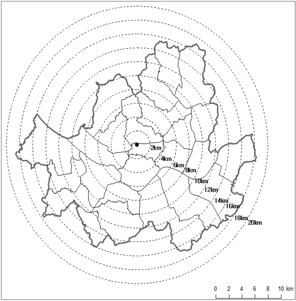
Figure 6.
Distribution of built-up area and green area according to the distance from Seoul’s city center.
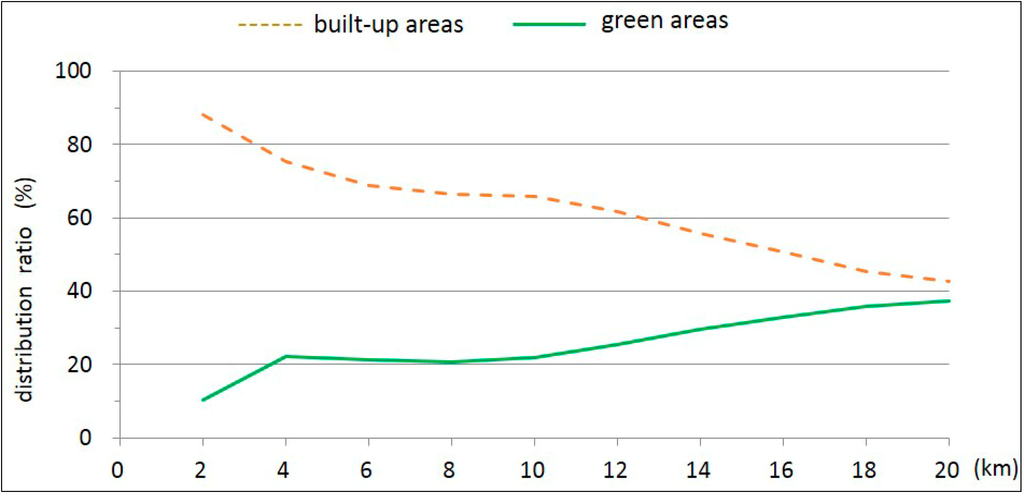
Figure 7.
Concentric circle of Seoul used to identify the built-up area and green area according to the distance from Seoul’s city center.
This concept can be explained with the following equation when the activity densities are approximated by population density. It can be seen that, even if the gross density of a city is the same, urban development has been carried out in a more compact way if the net density in the built-up areas is higher.
The higher the degree of city compactness, the greater the ratio of green area surrounding the built-up area. Accordingly, the ratio of green area for a total land area (i.e., the proportion of green areas) and the number of people within the built-up area (i.e., the net density) are employed as two complementary indicators that characterize urban compactness in this study. Total land area implies a separate, distinct administrative district. The type of land use in the built-up area is indicated according to plots used for building and factory construction according to the plot-based land-use classification system used in Korea. Meanwhile, the green areas indicate plots classified as forests, parks, and recreational areas.
As additional explanatory variables, population size as well as the presence of manufacturing industries and vehicle dependency are added. Population size is used to control for the absolute level of pollution emissions. The manufacturing dependency of a city is assessed as the net density of workers engaged in a manufacturing industry hiring five or more employees in the built-up area. Vehicle dependency is expressed as the interaction between vehicle ownership and availability of road infrastructure: Vehicle ownership is calculated as the number of registered motor vehicles per capita and road availability is represented as the proportion of the plots classified as road space and parking lot in the administrative district [45]. The data for these variables were obtained from the Statistical Yearbook (1997–2010) [43] and the Report of the Census on Establishments (1997–2010) [46], which were published by government agencies in each of the different cities.
3.2. Estimation Results
The FEM is selected based on the Hausman specification test [47], in which the estimated χ2 value is highly significant. The FEM is further divided into a one-way and a two-way model. The two-way FEM assumes that both the individual effect and the time effect have a constant influence over all observation units. Individual effects are caused by certain unique, unobservable properties of the 17 cities, while time effects are associated with the unique properties of each time series from 1996–2009. The production of air pollutants may be caused by certain unique and unobservable traits of individual cities. At the same time, air pollution control technologies and policies can potentially influence air quality in a mid- to long-term timeframe, and pollution may improve or worsen accordingly. Therefore, the two-way FEM is employed in order to control both individual (regional) effects and time effects. Time-Series Cross-Section Regression in SAS software (ver. 9.2) was used for estimation.
The estimation results summarized in Table 2, Table 3, Table 4, Table 5 and Table 6 indicate that urban compactness has both negative and positive effects on air quality; the former is about the spatial concentration of pollutants resulting from high densities in built-up areas, the latter is about the dispersion of pollutants attributed to green areas. On the one hand, NO2 and CO increased as the net population density increased, implying that compact urban development can result in greater spatial concentration of pollutants. On the other hand, SO2 and CO decreased as the proportion of green areas increased, implying that green areas secured by compact development can promote the dispersion of pollutants and thereby mitigate air pollution. Consequently, there is no clear impact of compact urban form on air quality. Air pollution resulting from compact urban development may vary according to pollutant-specific factors and emission source.
Table 2.
Panel data model estimates for urban characteristics and SO2.
| SO2 | Estimate | Std. Err | t-Value | Pr > |t| |
|---|---|---|---|---|
| Net density | 7.596 × 10⁻³ | 7.551 × 10⁻³ | 1.01 | 0.32 |
| Proportion of green area | −0.150 | 0.069 | −2.17 ** | 0.03 |
| Population | 4.930 × 10⁻⁶ | 0.000 | ||
| Manufacturing | 0.498 | 0.431 | 1.15 | 0.25 |
| Vehicle dependency | −31.530 | 24.800 | −1.27 | 0.20 |
| Intercept | 6.316 | 1.760 | 3.58 | 0.00 |
| N = 238, R2 = 0.828 | ||||
** p < 0.05
Table 3.
Panel data model estimates for urban characteristics and NO2.
| NO2 | Estimate | Std. Err | t-value | Pr > |t| |
|---|---|---|---|---|
| Net density | 0.190 | 0.109 | 1.74 * | 0.08 |
| Proportion of green area | 0.005 | 0.012 | 0.39 | 0.80 |
| Population | 7.739 × 10⁻⁶ | 0.000 | ||
| Manufacturing | 0.982 | 0.681 | 1.44 | 0.15 |
| Vehicle dependency | −35.480 | 39.100 | −0.91 | 0.37 |
| Intercept | 14.549 | 2.780 | 5.230 | 0.00 |
| N = 238, R2 = 0.810 | ||||
* p < 0.1
Table 4.
Panel data model estimates for urban characteristics and CO.
| CO | Estimate | Std. Err | t-Value | Pr > |t| |
|---|---|---|---|---|
| Net density | 1.302 | 0.580 | 2.25 ** | 0.03 |
| Proportion of green area | −13.720 | 5.310 | −2.58 ** | 0.01 |
| Population | −2.790 × 10⁻⁵ | 0.000 | ||
| Manufacturing | 7.137 | 33.100 | 0.22 | 0.83 |
| Vehicle dependency | −3484.950 | 1904.200 | −1.83 | 0.17 |
| Intercept | 79.970 | 13.540 | 5.91 | 0.00 |
| N = 238, R2 = 0.767 | ||||
*** p < 0.01; ** p < 0.05
Table 5.
Panel data model estimates for urban characteristics and O3.
| O3 | Estimate | Std. Err | t-Value | Pr > |t| |
|---|---|---|---|---|
| Net density | −0.040 | 0.074 | −0.59 | 0.55 |
| Proportion of green area | 9.10 × 10⁻³ | 8.13 × 10⁻³ | 1.12 | 0.26 |
| Population | 4.01 × 10⁻⁶ | 0.000 | ||
| Manufacturing | 0.092 | 0.464 | 0.20 | 0.84 |
| Vehicle dependency | −26.110 | 26.700 | −0.98 | 0.33 |
| Intercept | 27.700 | 1.900 | 14.59 | 0.00 |
| N = 238, R2 = 0.606 | ||||
Table 6.
Panel data model estimates for urban characteristics and PM10.
| PM10 | Estimate | Std. Err | t-Value | Pr > |t| |
|---|---|---|---|---|
| Net density | 0.228 | 0.725 | 0.31 | 0.75 |
| Proportion of green area | −43.387 | 29.927 | −1.45 | 0.15 |
| Population | 2.20 × 10⁻⁵ | 1.10E–05 | 2.05 ** | 0.04 |
| Manufacturing | 0.226 | 0.256 | 0.88 | 0.38 |
| Vehicle dependency | −727.525 | 431.900 | −1.68 | 0.11 |
| Intercept | 75.638 | 22.945 | 3.30 | 0.00 |
| N = 126, R2 = 0.698 | ||||
** p < 0.05
Meanwhile, urban compactness did not have a significant effect on PM10 and O3. Since O3 is not usually emitted directly into the air and is rather created by the chemical reactions of primary pollutants or previously emitted gases, it may be difficult to identify emission sources related to urban spatial structure. PM10 emissions are mainly caused by combustion of traffic and manufacturing, but it may also be hard to evaluate the influence of PM10 non-exhaust emissions on air quality. PM10 significantly increases with a growing number of people, indicating that, as city size increases, PM10 concentrations increase correspondingly. Manufacturing and vehicle dependency had no significant relationship with air pollution levels, although NO2 and CO are particularly related to automobile exhaust gases.
4. Conclusions
This study is intended to shed some light on whether compact urban development improves air quality or not. Considering that air pollution is influenced by spatial and temporal changes of urban characteristics as well as by the dispersion and dilution processes in the atmosphere, this study attempts to look into both the spatial concentration of pollutants by high-density development and the dispersion of pollutants by green open spaces. As seen in the spatial distribution patterns of air pollution, it is difficult to make the generalization that air pollution levels around city centers were increased by the spatial concentration of emission sources resulting from compact urban development. In regard to the effects of compact urban development on air pollution, the estimations of the panel data models indicate that urban compactness has both negative and positive effects on air quality. This study suggests that it is difficult to confidently assert that a compact city contributes to a reduction in air pollution; however, if compact urban development does contribute to a rising proportion of green areas, then such a development is helpful in mitigating air pollution.
Urban air pollution assessment is desirable in terms of determining the average concentration levels of an entire city rather than on a local scale. Because air pollution levels are influenced by the dispersion and dilution processes and the extent and magnitude of dispersion may depend upon spatial and temporal variations in urban characteristics, there is a need to differentiate in regard to whether emission sources are concentrated at the local or regional level and to develop an integrated management system that minimizes local to citywide emissions and thus regulates total urban emissions. For example, NO2 is emitted from sources linked to high densities and, therefore, local emission control measures are important. For PM10 and O3, it is preferable to monitor primary pollutants and sources overall and to regulate total emissions because these are most commonly produced by gas-to-particle conversions. Preferential controls and optional management strategies need to be followed in order to respond to changes in pollution levels, especially maximum concentrations for a certain period.
One of the limitations of this study is that it characterizes urban compactness using two simple measures—i.e., net density and proportion of green areas. Thus, it cannot reflect in a nuanced way the complex and diverse attributes of urban spatial structures (e.g., mixed land use, intensified city, etc.), which may also influence air pollution. The result of this study also does not take into account the significant value of green open spaces within built-up areas, since it considered only the value of outer green areas. Additional empirical analysis should be conducted to ascertain the extent to which green areas within built-up areas reduce air pollution.
Author Contributions
Hee-Sun Cho conceived the study and was involved in data analysis and manuscript writing. Mack Joong Choi directed and approved the study.
Conflicts of Interest
The authors declare no conflict of interest.
References and Notes
- Borrego, C.; Martins, H.; Tchepel, O.; Salmim, L.; Montiro, A.; Miranda, A.I. How urban structure can affect city sustainablili + 9 +/ty from an air quality perspective. Environ. Model. Softw. 2006, 21, 461–467. [Google Scholar]
- Environment Protection Agency. Our Built and Natural Environments: A Technical Review of the Interactions Between Land Use, Transportation and Environmental Quality; Environment Protection Agency: Washington, DC, USA, 2001. [Google Scholar]
- Frank, L.D.; Stone, B., Jr.; Bachman, W. Linking lands use with household vehicle emissions in the central puget sound: Methodological framework and findings. Transp. Res. Part D 2000, 5, 173–196. [Google Scholar]
- Nam, K.C.; Kim, H.S.; Son, M.S. A study on the correlation between compact of population and transport energy: An application of compact index. Korea Plan. Assoc. 2008, 43, 155–168. (In Korean) [Google Scholar]
- Stone, B., Jr.; Adam, C.; Mednick, T.H.; Scott, N.S. Is compact growth good for air quality? J. Am. Plan. Assoc. 2007, 73, 404–420. [Google Scholar] [CrossRef]
- Stone, B., Jr. Urban sprawl and air quality in larger US cities. J. Environ. Manag. 2008, 86, 688–698. [Google Scholar] [CrossRef]
- Thomas, L.; Cousins, W. The compact city: A successful, desirable and achievable urban form? In The Compact City: A Sustainable Urban Form; Jenks, M., Burton, E., Williams, K., Eds.; E&FN Spon: London, UK, 1996; pp. 53–65. [Google Scholar]
- Van der Waals, J.F.M. The compact city and the environment: A review. Tijdschr. voor Econ. Soc. Geogr. 2000, 91, 111–121. [Google Scholar]
- Breheny, M. Densities and sustainable cities: The UK experience. In Cities for the New Millennium; Eschenique, M., Saint, A., Eds.; Spon Press: London, UK; NewYork, NY, USA, 2001; pp. 39–51. [Google Scholar]
- Rudlin, D.; Falk, N. Building the 21st Century Home, the Sustainable Urban Neighborhood; Architecture Press: Oxford, London, UK, 1999. [Google Scholar]
- Tony, P.N. Environmental stress and urban policy. In Compact City: A Sustainable Urban Form; Jenks, M., Burton, E., Williams, K., Eds.; E&FN Spon: London, UK, 1996; pp. 200–211. [Google Scholar]
- Capello, R.; Camagni, R. Beyond optimal city size: An evaluation of alternative urban growth patterns. Urban Stud. 2000, 37, 1479–1496. [Google Scholar] [CrossRef]
- Kim, S.N.; Lee, K.H.; Ahn, K.H. The effects of compact city characteristics on transportation energy consumption and air quality. Korea Plan. Assoc. 2009, 44, 231–246. (In Korean) [Google Scholar]
- Chen, H.; Jia, B.; Lau, S.S.Y. Sustainable urban form for Chinese compact cities: Challenges of a rapid urbanized economy. Habitat Int. 2008, 32, 28–40. [Google Scholar] [CrossRef]
- Lyons, T.J.; Scott, W.D. Principles of Air Pollution Meteorology; Belhaven Press: London, UK, 1990. [Google Scholar]
- Mayer, H. Air pollution in cities. Atmos. Environ. 1999, 33, 4029–4037. [Google Scholar] [CrossRef]
- Briggs, D.J.; Collins, S.; Elliott, P.; Fishcher, P.; Kingham, S.; Lebret, E.; Pryl, K.; van Reeuwijk, H.; Smallbone, K.; van der Veen, A. Mapping urban air pollution using GIS: A regression-based approach. Int. J. Geogr. Inf. Sci. 1997, 11, 699–718. [Google Scholar] [CrossRef]
- Britter, R.E.; Hanna, S.R. Flow and dispersion in urban areas. Annu. Rev. Fluid Mechnics 2003, 35, 469–496. [Google Scholar] [CrossRef]
- Hanna, S.R.; Briggs, G.A.; Hosker, R.P. Handbook on Atmospheric Diffusion; DOE/TIC 11223, DE82–002045, Springfield, VA: NTIS/USDOC; United States Department of Energy: Washington, DC, USA, 1982. [Google Scholar]
- Roberts, P.T.; Fryer-Taylor, R.E.; Hall, D.J. Wind-tunnel studies of roughness effects on gas dispersion. Atmos. Environ. 1994, 28, 1861–1870. [Google Scholar] [CrossRef]
- Yoon, I.H. The Estimation of Air Quality Using the Surface Observation Data over South Korea. Ph.D. Thesis, Seoul National University, Seoul, Korea, 1991. [Google Scholar]
- Yeon, I.J.; Kim, K.Y. The investigation and estimate of influence on air quality by the exhaust of air pollutant from facility of the district heating located in small city. Korean J. Sanit. 2003, 18, 1–10. (In Korean) [Google Scholar]
- Fenger, J. Urban air quality. Atmos. Environ. 1999, 33, 4877–4900. [Google Scholar] [CrossRef]
- Hill, A.C. Vegetation: A sink for atmospheric pollutants. J. Air Pollut. Control. Assoc. 1971, 21, 341–346. [Google Scholar] [CrossRef] [PubMed]
- Chandler, T.J. Urban Climatology and Its Relevance to Urban Design; Technical Note 149; World Meteorological Organisation: Geneva, Switzerland, 1976. [Google Scholar]
- Wood, C.M. Air pollution control by land use planning techniques: A British-American review. Int. J. Environ. Stud. 1990, 35, 233–243. [Google Scholar] [CrossRef]
- Civerolo, K.; Hogrefe, C.; Lynn, B.; Rosenthal, J.; Ku, J.-Y.; Solecki, W.; Cox, J.; Small, C.; Rosenzweig, C.; Goldberg, R.; et al. Estimating the effects of increased urbanization on surface meteorology and ozone concentrations in the New York City metropolitan region. Atmos. Environ. 2007, 41, 1803–1818. [Google Scholar] [CrossRef]
- De Ridder, K.; Lefebre, F.; Adriaensen, S.; Arnold, U.; Beckroege, W.; Bronner, C.; Damsgaard, O.; Dostal, I.; Dufek, J.; Hirsch, J.; et al. Simulating the impact of urbansprawl on air quality and population exposure in the German Ruhr area. Part I: Reproducing the base state. Atmos. Environ. 2008, 42, 7059–7069. [Google Scholar]
- De Ridder, K.; Lefebre, F.; Adriaensen, S.; Arnold, U.; Beckroege, W.; Bronner, C.; Damsgaard, O.; Dostal, I.; Dufek, J.; Hirsch, J.; et al. Simulating the impact of urban sprawl on air quality and population exposure in the German Ruhr area. Part II: Development and evaluation of an urban growth scenario. Atmos. Environ. 2008, 42, 7070–7077. [Google Scholar]
- Cumulative effects are changes to the environment that are caused by an action in combination with other past, present and future human actions [31]. In other words, if various development projects are continuously undertaken on a broad scale, their effects will accumulate spatially and temporally, having a serious impact on the urban environment [32].
- Canadian Environmental Assessment Agency. Cumulative Effects Assessment Practitioners’ Guide. Available online: http://www.ceaa-acee.gc.ca/default.asp?lang=En&n=43952694-1&offset=6 (accessed on 11 September 2009).
- Oh, K.S.; Jeong, S.H.; Lee, D.K.; Jeong, Y.W. Environmental cumulative impacts of urban development of their assessment framework. Korea Plan. Assoc. 2006, 41, 147–161. (In Korean) [Google Scholar]
- The biggest and most congested part of a city where the majority of shops and businesses are located.
- Ministry of Environment. Republic of Korea. Annual Report on Ambient Air Quality (1997–2010). Available online: http://airemiss.nier.go.kr/main.jsp (accessed on 2 January 2012).
- An urban air quality monitoring network has been systematically measuring five classical pollutants’ concentrations in Korea from 1996, while 2009 is the most recent year for which data are available. At present, data on air pollution concentration is available until 2012 but it is not easy to obtain variables representing urban characteristics such as population, manufacturing, and transportation to be used in the panel data model analysis afterwards. One of the 17 cities was created from three cities (one coastal and two inland cities) in 2010, meaning it is difficult to ensure consistent data in that case. Thus, data for the period 1996–2009, which at the time consisted of the most recent research data, were used.
- Seoul, Busan, Incheon, Daegu, Gwangju, Ulsan, Daejeon, Suwon, Bucheon, Ansan, Wonju, Cheongju, Gunsan, Gumi, Pohang, Yeosu and Masan.
- Seoul, Busan, Incheon, Daegu, Gwangju, Ulsan, Daejeon, Suwon and Bucheon.
- Land cover map published by MoE. Available online: http://egis.me.go.kr (accessed on 18 July 2014).
- For gas-phase pollutants, the number of air monitoring stations ranged from 70 in 1996 to 124 in 2009, while PM10 was monitored in 23 rising to 97 stations for the same years.
- Gaseous pollutant concentrations are expressed as ppb (parts per billion) and PM10 is expressed as µg/m3. The distance from the city center to the air quality monitoring stations is measured in kilometers.
- Baltagi, B.H. Econometric Analysis of Panel Data; John Wiley & Sons, Inc.: New York, NY, USA, 2008. [Google Scholar]
- Ashenfelter, O.; Levine, B.P.; Zimmerman, J.D. Statistics and Econometrics: Methods and Applications; John Wiley & Sons, Inc.: New York, NY, USA, 2003. [Google Scholar]
- Korean Statistical Information Service. Statistical Yearbook (1997–2010). Available online: http://www.kosis.kr/ (accessed on 27 March 2012).
- Gujarati, D.N.; Porter, D.C. Basic Econometrics, 5th ed.; McGraw Hill: New York, NY, USA, 2009. [Google Scholar]
- The units of overall explanatory variables are as follows: net density (number of persons/km2), proportion of green areas (%), population size (number of persons), manufacturing (number of workers/km2), and vehicle dependency (number of vehicles/number of persons) is described in the following equation: .
- Korean Statistical Information Service. Report of the Census on Establishments (1997–2010). Available online: http://www.kosis.kr/ (accessed on 27 March 2012).
- Greene, W.H. Econometric Analysis; Prentice Hall: Upper Saddle River, NJ, USA, 1997. [Google Scholar]
© 2014 by the authors; licensee MDPI, Basel, Switzerland. This article is an open access article distributed under the terms and conditions of the Creative Commons Attribution license (http://creativecommons.org/licenses/by/3.0/).