Abstract
As one of the most effective traffic demand management opinions, congestion pricing can reduce private car travel demand and the associated carbon dioxide emissions. First, we summarized the status quo of transport carbon dioxide emission charges and congestion pricing, and then, we analyzed the characteristics of urban transport carbon dioxide emissions. Then, we proposed a (pricing) framework in which carbon emission costs would be considered as part of the generalized cost of travel. Based on this framework, this paper developed a bi-level mathematical model to optimize consumer surplus, using congestion and carbon emission charges as the control variables. A dissect search algorithm was used to solve the bi-level program model, and a numerical example was given to illustrate the methodology. This paper incorporates the emission pricing into the congestion pricing model, while considering two modes, and puts forward suitable proposals for the implementation of an urban traffic congestion pricing policy in China.
1. Introduction
With rapid social and economic development, urbanization improves people’s living standards. However, at the same time, it leads to a rapid increase in the urban traffic demand. Today, traffic congestion has become a critical problem faced by many big cities worldwide. Even the rapid growth of urban infrastructure construction is far behind the growth rate of urban car ownership and travel demand. Traffic congestion has severe societal and economic effects. Moreover, the rapid development of urban transportation demand also imposes an adverse impact on the urban surroundings and the living environment. The greenhouse emissions (e.g., carbon dioxide) have significantly increased in the past few decades. Across all sectors of the society, transportation contributes a large proportion of emissions, and this proportion is still undergoing a fast growth. According to the 2009 report, “Transport, Energy and carbon dioxide: Towards Sustainable Development,” by the International Energy Agency, the carbon dioxide emissions from transportation occupy about 25% of the total [1]. In recent years, urban carbon dioxide emissions have gradually caused widespread concerns [2,3,4,5].
In 2009, carbon dioxide emissions from China’s transportation industry were about 540 million metric tons, accounting for about 8.2% of its national total emissions. Although the total amount is not large, it is one of the fastest growing areas. Carbon dioxide emissions from urban passenger transportation are about 134.25 million metric tons, accounting for 2.3% of its national total emissions (about 5.8 billion tons) and 24.5% of those from transportation. Among them, the proportions from buses, cars and taxis are 31%, 34.8% and 34.2% respectively. Overall, carbon emissions from urban passenger transportation accounted for 30.6% of the total emissions of urban traffic, and carbon emissions of urban transport (including urban freight transport) accounted for 73.8% of the total emissions of the transportation industry [6]. Similarly, in 2011, carbon dioxide emissions from the USA transportation sector accounted for 32% of its national total or, equivalently, 7% of global emissions. Cars and trucks accounted for 73%, reaching 270 million tons per year.
Different travel modes perform very differently in terms of carbon dioxide emissions. It is estimated that if we rank the typical modes in the urban passenger transport system according to their carbon dioxide emissions intensity, from high to low, the corresponding sequence is taxi, private car, motorcycle, bus, bus rapid transit, rail transportation, bicycle and walking. Therefore, raising the portion of public transportation in urban areas will greatly facilitate passenger transport energy conservation and reduce carbon dioxide emissions.
Traffic demand management (TDM) policies aim to reduce unnecessary private car travel demand and encourage more efficient, environmental protecting and energy-saving modes, such as public transportation, walking and bicycle modes. Steg and Vlek had divided TDM into two “pull” and “push” categories [7]; as one of the push measures, congestion pricing not only makes travelers cut car use and turn to public transport and bicycle modes [8,9,10], but also reduces the external costs of urban passenger transportation, including traffic congestion, air pollutant emissions and incidents [11,12,13].
To relieve urban traffic congestion and reduce carbon dioxide emissions, we propose an integrated pricing strategy where carbon emission costs are considered as part of the generalized traveler costs. The impositions of such costs will change travelers’ choices over the travel mode and route, such that traffic congestion and CO2 emissions can be reduced. The strategy aims at achieving the following targets: (1) reduce traffic pollution and greenhouse emissions to improve urban air quality; (2) balance transportation supply and demand to ease the traffic demand pressure on urban centers and facilitate overall network equilibrium; and (3) divert travelers from private transport modes to public transport modes and, in so doing, enhance the overall social welfare.
The paper is organized as follows. Section 2 reviews the urban transport carbon emissions and congestion pricing development. In Section 3, we analyze traveler behavior change under the congestion pricing policy. In Section 4, the bi-level programming model is presented in detail. Section 5 is the case study and discussion. Finally, we conclude this paper in Section 6.
2. Literature Review
In recent years, urban transport carbon emissions and congestion pricing have been studied intensively worldwide. In the urban road passenger transport system, Ferrari proposed a price mechanism that aims to minimize the generalized cost of the entire urban transportation system and balance the transportation system supply and demand. The mathematical model included congestion pricing, passenger transport fares and service levels as the decision variables and considered network traffic, budget, environment as the constraints [14]. Chen et al. conducted a quantitative study of carbon emissions in the context of a low carbon city for the urban transport sector in Shanghai. Traveler choices among various modes of transportation are considered [15]. Ubeda et al. studied a logistics management system and found that changes in management measures will affect the vehicle carbon dioxide emissions per vehicle load-distance [16]. As such, we can generally calculate the carbon dioxide emissions based on the vehicle fuel consumption or distance traveled. To analyze the effect of a carbon-based congestion pricing scheme on the traveler model split, Meng and Liu adopted a binary logit model to represent a bi-modal transportation network composed by the car and rail modes [17].
For the study of a carbon tax, Pigou believed that government intervention (e.g., in the form of taxes or subsidies) was necessary to internalize the external costs of the traveler and to improve the environment [18]. By analyzing the effect of a carbon tax on carbon dioxide emissions from energy-related industries, Floros and Vlachou concluded that a carbon tax can reduce carbon dioxide emissions effectively [19]. Greedy and Sleeman analyzed the relationship between a carbon tax and social welfare and concluded that a carbon tax would lead to only a small excess marginal cost [20]. Yusuf and Resosudarmo took Indonesia as an example to analyze the effect of a carbon tax in developing countries using a computable general equilibrium (CGE) model [21]. Hammar and Jagers tested the CO2 tax increase effects on the emission reduction in Sweden and found that car use frequency is the relative key factor of the fairness principle [22]. Giblin and McNabola modeled the introduction of carbon-based taxes in Ireland, and the results indicated that this tax would reduce the CO2 emissions intensity by 3.6%–3.8% [23]. Fu and Kelly also evaluated the adoption of carbon-related tax impacts in Ireland and declared that this fuel-based carbon tax might reduce 1.75%–3.82% of the CO2 emissions, depending on the scenario [24].
In China, research has achieved more progress in the congestion pricing theory. Wang et al. (2003) conducted a detailed survey on the development process and cutting-edge dynamics of congestion pricing theory [25]. Chen and Zhang established a bi-level programming model and used a genetic algorithm to solve the model [26]. Xing qualitatively incorporated the external traveler cost from crowding into a pricing model [27]. Liu considered the congestion pricing of an urban road system and analyzed the second best congestion pricing in a multi-period and multi-user framework, the established bi-level programming model, where the upper planning level aims to maximize social welfare, while the lower-level is a general road network equilibrium model (with multiple periods and multiple users) [28]. Although the theoretical study of congestion pricing in China is relatively mature, practical implementation is very scarce.
Based on the theory of a carbon dioxide carbon tax, the carbon emissions quantitative models of the different transportation modes in urban transportation can be as shown as:
where:
Fi = Qiectax = ectaxeipili × 10-3
- i, traffic travel mode;
- Fi, carbon dioxide emission charges value in the i-th travel mode (Yuan);
- Qi, carbon dioxide emissions in the i-th travel mode (ton);
- ectax, domestic carbon tax standards (Yuan/ton);
- ei, carbon dioxide emissions intensity in the i-th travel mode (kg/person/km);
- pi, the average occupancy number in the i-th travel mode (person);
- li, distance in the i-th travel mode (km);
Table 1 summarizes the carbon dioxide carbon tax rate in different countries [29,30]. In China, the carbon tax is also discussed by the academic world, but has not been put into practice as congestion pricing.

Table 1.
Carbon dioxide carbon tax in different countries.
| Country | Carbon Dioxide Carbon Tax (Yuan/ton) | |
|---|---|---|
| Finland | 150.25 | |
| Sweden | 943.95 | |
| Netherlands | 19.44 | |
| Canada-Quebec | 329.15 | |
| Japan | 187.59 | |
| China | Wei (2002) | 31.4~62.8 |
| Ministry of Finance | 10 | |
| Ministry of Environmental Protection | 20 | |
Although quite a bit of research on carbon emissions charges and congestion pricing has been done, there are still inadequacies. First, existing studies have not targeted the quantitative estimation of the urban transport carbon dioxide emissions in the carbon emission charges model. Second, existing studies did not consider the impact of congestion pricing in urban transport carbon dioxide emission charges. The paper hence aims to fill this gap by integrating carbon emission charges (based on carbon emission indices and influencing factors) into a congestion pricing model. The charges for carbon emissions are implemented in this modeling framework to relieve urban traffic congestion and reduce carbon emissions.
The integration of congestion pricing and carbon charges not only reflects the generalized cost of road transportation and reduces private car usage, but also, it decrease CO2 emissions and enhances social welfare, to achieve more environmental protection and energy savings development. Meanwhile, the proposed suggestions on the implementation of carbon charges are also useful for government decision making and public acceptance of carbon charge policy.
3. Generalized Travel Cost Analysis
To reduce urban transportation carbon dioxide and to solve the problem of urban traffic congestion, here, we expand the generalized travel costs of the traveler. That is, the generalized travel costs change under normal circumstances through the collection of the cost of carbon emissions, as well as congestion costs.
For car travelers, the travel costs mainly include travel time costs, operating expenses, the additional costs of traffic congestion and carbon emission costs. For bus travelers, the travel costs include travel time costs, bus fares and the carbon emission costs.
According to the carbon emission charge model in Section 2 and related content, we can express the generalized travel costs of the various sections of car travel and bus travel as follows (the variables without a ^ relate to car and with ^ relate to bus):
 Where:
car: Ca(xa) = ta(xa) ̸ γ1 + la · Opri + ua + ectaxe1p1la × 10-3
- ta(xa), the average travel time for a vehicle on link a when trips are xa (h);
- xa, the trips on link a (vehicle/h);
- la, length of link a (km);
- γ1, γ2, conversion factor between money and time of car and bus (h/Yuan);
- Opri, running costs of car in link a (Yuan/km);
- ua, congestion costs in link a (Yuan);
- Ŷ, bus fare (Yuan).
In Formula (2) and Formula (3), we need to impose the cost of carbon emissions for a single traveler. For the car travelers, this paper argues that the cost of carbon emissions can be levied by the amount of consumed fuel. For bus travelers, the most direct method is to adjust the bus fares according to the offset of the carbon emission charges in the process of bus travel.
4. Congestion Pricing Bi-level Programming Model Considering the Cost of Carbon Emissions
4.1. Basic Assumptions
The study was carried out using the following assumptions:
 where:
- (1)
- The congestion pricing is only imposed on the car traveler. The congestion pricing model ignores non-motorized travel modes, such as walking and bicycle; the paper only considers car trips and bus travel in the model building process and ignores the traveling status impact between them;
- (2)
- The travel mode and the path of all travelers are the most economical, which means that they choose the least cost mode and route;
- (3)
- The period of the proposed model is the morning or evening peak period of urban traffic and considers the traffic demand as a known deterministic demand;
- (4)
- The paper uses the generalized cost function to calculate the travel costs (as shown in Formulas (2) and (3));
- (5)
- The link travel time function is the BPR (Bureau of Public Roads) function developed by the American Road Bureau [31].
- ta(xa), the average travel time for a vehicle on link a when trips are xa;
 , free flow travel time on link a;
- C, road capacity of link a;
- α, β, parameters.
4.2. Symbols Definition
Here, we use symbols to signify the general road network G = (N, A) of vehicles. Table 2 presents all the variables and their definitions.
Table 2.
Variables and their definitions.
| Variables | Definitions |
|---|---|
| N | the collection of network nodes |
| A | the collection of the arc (sections) in the network |
| a | a link in the network, a∈ A |
| R | the collection of starting nodes generated to travel, R ⊆ N |
| S | the collection of destination nodes attracted to travel, S ⊆ N |
| r | a starting node, r ∈ R |
| s | a final destination node, s ∈ S |
| qrs | the total trips from r to s of the study period |
| qrs | the car trips from r to s of the study period |
 | the bus trips from r to s of the study period |
| xa | car trips on link a |
 | bus trips on link a |
 | vehicle travel time on link a |
| ta (●) | car travel time on link a ta =ta(xa) |
 | bus travel time on link a  |
| ѱrs | the set of all paths connecting OD (Origin Destination) pair r-s |
 | car trips in the path k among the OD pairs r-s, k ∈ ѱrs |
 | bus trips in the path k among the OD pairs r-s, k ∈ ѱrs |
 | the total travel time(impedance) of car in the path k among the OD pairs r-s, k ∈ ѱrs |
 | the total travel time(impedance) of car in the path k among the OD pairs r-s, k ∈ ѱrs |
| ua | congestion costs of car on link a (Yuan) |
 | 0-1 variable, if link a is in the path k among the OD pairs r-s, then  = 1, otherwise = 0 = 1, otherwise = 0 |
| prs | the total travel demand among the OD pairs r-s (person)  |
| prs | car travel demand among the OD pairs r-s (person) |
 | bus travel demand among the OD pairs r-s (person) |
| μrs | the minimum travel cost of car travel among the OD pairs r-s (Yuan) |
 | the minimum travel cost of bus travel among the OD pairs r-s (Yuan) |
4.3. The Lower Level of the Bi-Level Programming Model
The user mode choice behavior is described in the lower level of the bi-level programming model. A logit model is used to represent the market share proposition. The different modes of transportation route choice behavior also meet the Wardrop User Equilibrium Principle. Therefore, here, we establish a combined model of transportation mode choice and traffic assignment based on network equilibrium distribution in the conditions of the congestion charge. Ignoring the interaction between bus and car traffic, we develop the corresponding mathematical model aiming to minimize the generalized travel cost. The objective function and the constraints are shown in Formula (5).


In Formula (5), constraints 1 to 3 describe the conservation of the relationship between the various ways of OD (Origin Destination) trips and path trips. Constraints 4 and 5 are variable non-negative constraints; Constraints 6 to 7 are the link trips’ expression.
The lower level of the bi-level programming model obeys the Wardrop User Equilibrium Principle; it ensures the travel distribution for two-way travel to meet the logit model assignment. For solving the lower user model, the paper uses the successive averages algorithm.
4.4. The Upper Level of the Bi-Level Programming Model
The traffic management decision-making behavior is represented in the upper level of the bi-level programming model. Here, we suppose that the city’s traffic management aims to maximize the surplus (CS) (customer surplus) of all travelers (car trips and bus travelers); that is, transportation planning managers develop a pricing strategy to achieve the following purpose, when considering user response to the pricing strategy and the case of link trips not exceeding the capacity, maximizing the user surplus in the whole system. The user surplus, CS, is equal to the margin between the entire transportation system user benefits TUB (total user benefit) and the total cost of TSC (total social cost), namely:

Therefore, the upper model can be expressed as:
 where:
- Ca, road capacity of car on link a (pcu/h) (pcu: passenger car unit);
- Ĉa, road capacity of bus vehicle on link a (pcu/h);
- p, car average occupancy number (person);
 , bus average occupancy number (person);
4.5. Model Solution Method
The solution of the bi-level programming model for the transport sector is very complex. One reason is that the bi-level programming problem is an NP-hard (Nondeterministic Polynomial) problem [32]. On the other hand, the bi-level programming problems are generally non-convex. Therefore, it is usually only possible to find a local optimal solution rather than the global optimal solution. Many scholars have developed a variety of algorithms for the practical conditions, the calculation accuracy and computational complexity of each method, but the calculation accuracy and computational complexity is not the same.
The paper uses a direct search algorithm based on the step acceleration method and the penalty function method to solve the bi-level programming model of congestion pricing considering the cost of carbon emissions [32,33].
The main work of the direct search algorithm is to solve the upper level model, and the lower level can serve as the constraints of the upper level. Here, we adopted the penalty function method to transfer the upper level model into the minimum problem (see Equation 8) and then used the step acceleration method to solve this problem.

For a determined penalty factor γ > 0, we used the step acceleration method to solve the model (9), that is to determine an initial set of congestion pricing scheme u to search. Under this congestion pricing scheme, we solved the lower level model (6) and obtained the car trips and bus trips in each road sections, and these results are fed back to the upper level model (9). Then, we re-use the successive average method to determine the iteration steps, until the cycle results meet the penalty γ conditions and acquire the congestion pricing scheme, also to ensure that road traffic volume cannot exceed the road section capacities. If not, we increase the penalty factors and iterations to calculate the optimal solution of the bi-level program model.
The algorithm steps are as follows:
- Step 0: (Initialization). Let the initial penalty factor γi, here i = 1.
- Step 1: (Initial assignment). Determine an initial set of congestion pricing schemes u(0) = 0, where u = u(0), to solve the user equilibrium assignment model of the lower level, and calculate the value of x0 and q0. Then, put these values in the upper level model, Z(ua, γ), and choose the initial step length, δ, and acceleration factor, σ, where j = 1, k = 0(j = 1,2,…,n).
- Step 2: (Direction searching). Let u* = u(0) + βδej; here, ej is a unit vector; the j-th element of ej is one, and the other elements are zero. Let β =1 to solve the lower level model, and calculate the objective of the upper level model, Z(u*, γ). If Z(u*, γ) < Z(u(0), γ), then the value of β is not changed; otherwise, β = −1. If Z(u*, γ) > Z(u(0), γ), then let u* = u(0) and j = j + 1, and go to Step 2.
- Step 3: (Mode searching). If Z(u*, γ) < Z(u(k), γ), then let u(k+1) = u*, Z(u*, γ) = Z(u(k+1), γ),
 , j = 1, k = k + 1, and go to Step 4; otherwise, let δ < ε, and go to step 2.
 - Step 4: (Stop criterion check). If xa > Ba, ∀a, increasing the penalty factor γi, let γi+1 = λγi(λ > 1), where i = i + 1, u(0) = u(k), and go to Step 1. Otherwise, the stop and output congestion pricing, uk, is the optimal solution.
5. Numerical Example
5.1. Basic Parameters Setting
In this section, we present the basic parameter setting of the case study, Figure 1 a was the partial road network of Harbin, and the simplified road network for the numerical example is shown in Figure 1 b. There are six nodes and seven road sections in this road network; here, we assumed that the node origin-destination pairs were nodes (1, 3) and (2, 4).
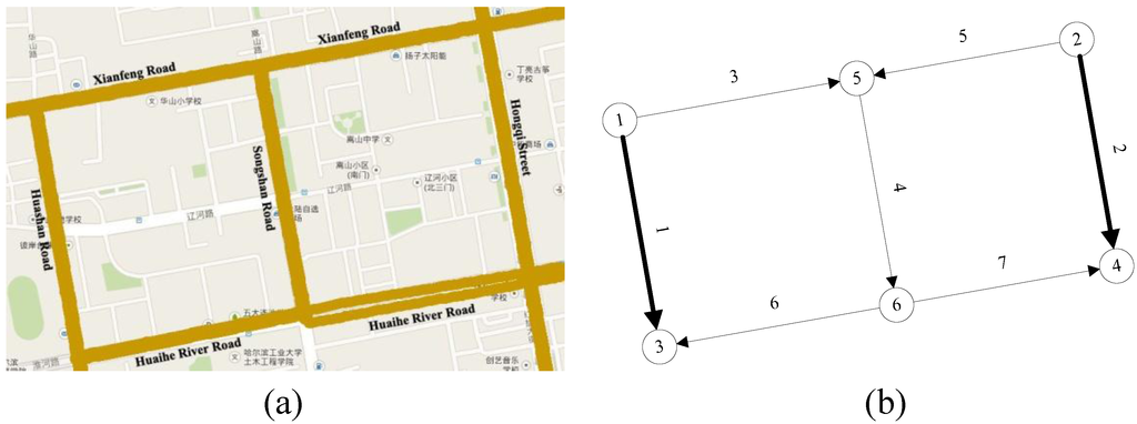
Figure 1.
Topology of the urban road network example in Harbin.
The length of the various road links, road capacity, as well as free travel time and other parameters of the case are shown in Table 3 and Table 4, the total traffic demand of two OD pairs (1, 3) and (2, 4) are assumed to be 3,800 and 5,000, respectively. Here, we ignore the intersection delay and interaction between two types of vehicle.
Table 3.
Some parameter values in model.
| Parameter | α | β | γ1 | γ2 | Opri | Ŷ |
| Value | 0.15 | 4 | 2 | 2 | 1 | 1 |
| Parameter | ectax | e1 | e2 | p1 | p2 | |
| Value | 50 | 0.2 | 0.069 | 1 | 25 |
Table 4.
Road length, free passage of time and link capacity in the road network.
| Link | 1 | 2 | 3 | 4 | 5 | 6 | 7 |
|---|---|---|---|---|---|---|---|
| la/km | 0.61 | 0.61 | 0.55 | 0.61 | 0.55 | 0.55 | 0.55 |
| /min | 1.20 | 1.20 | 0.75 | 1.20 | 0.75 | 0.75 | 0.75 |
| Car Ca (pcu/h) | 2,600 | 3,290 | 2,430 | 3,290 | 2,600 | 2,430 | 2,430 |
| Bus Ĉa (pcu/h) | 1,730 | 2,190 | 1,620 | 2,190 | 1,730 | 1,620 | 1,620 |
5.2. Results Analysis
The congestion pricing standards were changed by 0.5 Yuan per step, using the MATLAB software and the model algorithm to solve the model. The calculated numerical results are shown in Table 5 and Table 6, which included the total travel cost in two ways and carbon dioxide emissions in two ways under different congestion pricing schemes, respectively.
Table 5.
The total travel cost in two-way travel under different congestion pricing scheme (unit).
| u1 = 0.0 | u1 = 0.5 | u1 = 1.0 | u1 = 1.5 | u1 = 2.0 | |
|---|---|---|---|---|---|
| u2 = 0.0 | 12,062 | 11,182 | 10,863 | 10,941 | 11,177 |
| u2 = 0.5 | 10,883 | 10,003 | 9,684 | 9,762 | 9,998 |
| u2 = 1.0 | 10,451 | 9,571 | 9,252 | 9,330 | 9,566 |
| u2 = 1.5 | 10,550 | 9,670 | 9,351 | 9,428 | 9,664 |
| u2 = 2.0 | 10,859 | 9,979 | 9,660 | 9,737 | 9,972 |
Table 6.
Carbon dioxide emissions in two-way travel under different congestion pricing schemes (kg).
| u1 = 0.0 | u1 = 0.5 | u1 = 1.0 | u1 = 1.5 | u1 = 2.0 | |
|---|---|---|---|---|---|
| u2 = 0.0 | 976 | 959 | 934 | 902 | 866 |
| u2 = 0.5 | 953 | 935 | 910 | 878 | 842 |
| u2 = 1.0 | 920 | 902 | 877 | 845 | 809 |
| u2 = 1.5 | 878 | 860 | 835 | 803 | 767 |
| u2 = 2.0 | 831 | 813 | 788 | 756 | 719 |
From Table 5 and Table 6, we can draw these opinions:
- (1)
- For u1 = 1, u2 = 1, the upper objective function, Z, has the smallest value, that is the minimum total travel cost is 9,252 units. Compared to the value of 12,062 units for u1 = u2 = 0, it reduces the total cost by 2,810 units, which means 23.3% of the total travel cost.
- (2)
- Carbon dioxide emissions monotonically decreased in the test road network, because of the different passengers’ travel emission intensity of carbon dioxide emissions. With the congestion pricing standard imposed on the link increased, more car passengers changed their mode and chose the bus, and the carbon dioxide emissions trended in decreasing manner. When u1 = 1, u2 = 1, the total carbon dioxide emissions in the road network was 877 kg.
- (3)
- Figure 2 shows the passenger demand of each road section before and after the implementation of congestion pricing. When u1 = 1, u2 = 1, travel trip transfer amounts from car to bus were 856 trips and 1,114 trips on link 1 and link 2, respectively, the saturations of road link 1 and link 2 changed from 0.83, 0.86 to 0.46, 0.48, respectively; the level of service changes significantly.
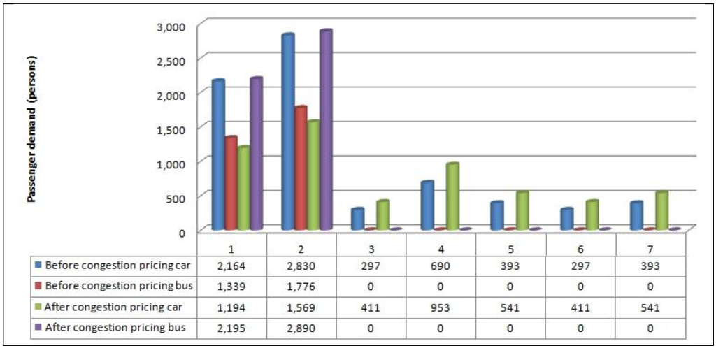 Figure 2. Passenger demand of each road section before and after congestion pricing.
 - (4)
- Figure 3 shows the carbon dioxide emissions of each road section before and after the implementation of congestion pricing. When the total travel cost is minimized, carbon dioxide emissions of the car and bus models are 623 kg and 214 kg, respectively. Compared to 845 kg and 131 kg when not imposing congestion pricing, carbon dioxide emissions of cars reduce by 182 kg, and carbon dioxide emissions of buses increase by 83 kg. The total reduction of the carbon dioxide emissions is 99 kg, a 10.1% reduction.
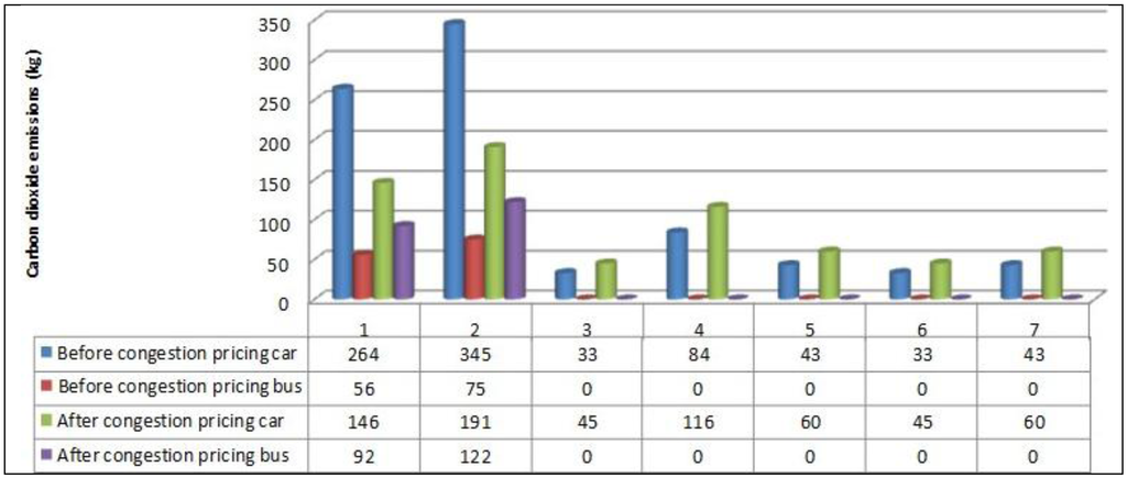
Figure 3.
Carbon dioxide emissions of each road section before and after congestion pricing.
5.3. Discussions of the Results
With the development of electronic and information communication technology, the technical issue is not the obstacle of the implementation of congestion pricing and carbon tax policy. Public acceptance is the key factor for the implementation of congestion pricing and carbon tax.
The successful experience of Singapore [34], London [35] and Stockholm [36] has shown that the trial of congestion pricing, re-allocation of revenue and public survey will make the public raise support and acceptance of this economic policy by feeling the benefits of congestion pricing, such as less congestion, cleaner air and less energy consumption. Existing research shows two different opinions on congestion pricing revenue re-allocation; one is the improvement of transportation infrastructure facilities and public transportation services [37,38]; another is the compensation of travelers, such as tax decreases and subsidies [39,40].
As shown in Figure 3, the implementation of a congestion pricing policy will change the proportion transferring from private car to bus, so that the transportation management authority should also consider the following measures, such as bus route re-planning, park and ride facility setting and the bus service frequency re-scheduling.
The quantitative estimation of carbon emissions and measuring the impact of carbon emissions charges can effectively reduce the total system travel cost and carbon dioxide emissions. The proposed model can alleviate the problem of urban traffic congestion and reduce carbon emissions to a certain extent, achieving more environment protection and lower carbon development. The public transportation mode share will increase for car travelers who choose the bus, which can also improve service level of the road network.
Meanwhile, the integration of different urban transportation economic measures will achieve the sustainable development of the urban passenger transportation market [12]. The integration of congestion pricing, parking fees, public transportation fares and oil price will realize a synergistic effect, not only reducing private car usage and congestion, but also increasing public transportation ridership and social welfare [41,42].
6. Conclusions
This paper proposes a pricing scheme that considers carbon dioxide emissions, as well as congestion externality and that can relieve urban traffic congestion and reduce carbon dioxide emissions. A numerical example is used to verify the feasibility of this model. From the case study analysis, also, we presented some useful information.
By adopting a bi-level programming model to optimize the congestion pricing and carbon emission charges, this paper incorporated the emission pricing into the congestion pricing model while considering two modes. In the upper level, the user surplus is maximized; while in the lower level, the equilibrium conditions for both car and bus with a logit model as the market share are solved. Using a small part of the road network of Harbin, China, the real-world implementation and implications have been examined.
The integration of urban road congestion pricing and carbon emission charges will help us to achieve the sustainable development of urban road transportation. Kim et al. (2013) have indicated that the fairness of the road pricing and environmental taxation is the most influential factor for people to accept both pricing schemes [43]. Therefore, research on public acceptance and public support for congestion pricing and carbon emission charges will be an interesting research direction.
The effect of relaxing the fixed demand assumption on the results can be an interesting addition to the study. One of the main effects of congestion pricing is to reduce or shift the peak demand. This addition can be done using simplified assumptions, like iterative demand updating based on the new general costs of travel for each OD pair. Meanwhile, in the future, we will pay more attention to the social costs of bus operation and divide it into the kinds of time, including access time, waiting time, traveling time and transfer time.
Acknowledgments
This research is supported by the National Natural Science Foundation of China (Project No. 71073035 and No. 71203045), the Program for New Century Excellent Talents in University (NCET-10-0065) and the China Postdoctoral Science Foundation funded project (No. 2013M540299). The authors would like to express their sincere thanks to the anonymous reviewers for their helpful comments and valuable suggestions on this paper.
Author Contributions
Jian Wang had conceived and designed the study, Libing Chi had analyzed the data, Xiaowei Hu had drafted and revised this manuscript, and Hongfei Zhou had collected the data.
Conflicts of Interest
The authors declare no conflict of interest.
References
- IEA. Transport, Energy and CO2: Moving towards Sustainability; International Energy Agency: Paris, France, 2009. Available online: http://www.iea.org/publications/freepublications/publication/transport2009.pdf (accessed on 15 April 2012).
- Stead, D. Relationships between transport emissions and travel patterns in Britain. Transp. Poli. 1999, 6, 247–258. [Google Scholar] [CrossRef]
- Richardson, B.C. Sustainable transport: Analysis frameworks. J. Transp. Geogr. 2005, 13, 29–39. [Google Scholar] [CrossRef]
- Lefèvre, B. Long-term energy consumptions of urban transportation: A prospective simulation of “transport–land uses” policies in Bangalore. Energ. Poli. 2009, 37, 940–953. [Google Scholar] [CrossRef]
- Santos, G.; Behrendt, H.; Maconi, L.; Shirvani, T.; Teytelboym, A. Part I: Externalities and economic policies in road transport. Res. Transp. Econ. 2010, 28, 2–45. [Google Scholar] [CrossRef]
- Zhu, Z.; Zhao, J.; Zhang, X. Urban Road Traffic and Energy Conservation. Urban Roads Brid. Flood Cont. 2008, 10, 46–47. (in Chinese). [Google Scholar]
- Steg, L.; Vlek, C. The role of problem awareness in willingness-to change car use and in evaluating relevant policy measures. In Traffic and Transport Psychology; Rothengatter, J.A., Carbonell Vaya, E., Eds.; Pergamon Press: Oxford, UK, 1997; pp. 465–475. [Google Scholar]
- Eriksson, L.; Nordlund, A.M.; Garvill, J. Expected car use reduction in response to structural travel demand management measures. Transp. Res. Part F 2010, 13, 329–342. [Google Scholar] [CrossRef]
- Habibian, M.; Kermanshah, M. Exploring the role of transportation demand management policies’ interactions. Scie. Iran. A 2011, 18, 1037–1044. [Google Scholar] [CrossRef]
- De Palma, A.; Lindsey, R. Traffic congestion pricing methodologies and technologies. Transp. Res. Part C 2011, 19, 1377–1399. [Google Scholar] [CrossRef]
- Lautso, K.; Spiekermann, K.; Wegener, M. Propolis: Planning and Research of Policies for Land Use and Transport for Increasing Urban Sustainability. Available online: http://www.cipra.org/alpknowhow/publications/propolis/ (accessed on 31 May 2013).
- Santos, G.; Behrendt, H.; Teytelboym, A. Part II: Policy instruments for sustainable road transport. Res. Transp. Econ. 2010, 28, 46–91. [Google Scholar] [CrossRef]
- Ong, H.C.; Mahlia, T.M.I.; Masjuki, H.H. A review on emissions and mitigation strategies for road transport in Malaysia. Renew. Sustain. Energ. Reviews 2011, 15, 3516–3522. [Google Scholar] [CrossRef]
- Ferrari, P. A model of urban transport management. Transp. Res. Part B 1999, 33, 43–61. [Google Scholar] [CrossRef]
- Chen, F.; Zhu, D.; Xu, K. Research on urban low-carbon traffic model, current situation and strategy: An empirical analysis of Shanghai. Urban Plan. Forum 2009, 6, 39–46. (in Chinese). [Google Scholar]
- Ubeda, S.; Arcelu, J.; Faulin, J. Green logistics at Eroski: A case study. Int. J. Prod. Econ. 2011, 131, 44–51. [Google Scholar] [CrossRef]
- Meng, Q.; Liu, Z. Impact analysis of cordon-based congestion pricing on mode-split for a bimodal transportation network. Transp. Res. Part C 2012, 21, 134–147. [Google Scholar] [CrossRef]
- Pigou, A.C. The Economics of Welfare, 4th ed.; Macmillan: London, UK, 1920. [Google Scholar]
- Floros, N.; Vlachou, A. Energy demand and energy-related CO2 emissions in Greek manufacturing: Assessing The impact of A carbon tax. Energ. Econ. 2005, 27, 387–413. [Google Scholar] [CrossRef]
- Greedy, J.; Sleeman, C. Carbon taxation, prices and welfare in New Zealand. Ecol. Econ. 2006, 57, 333–345. [Google Scholar] [CrossRef]
- Yusuf, A.A.; Resosudarmo, B.P. Does clean air matter in developing countries’ megacities? A hedonic price analysis of the Jakarta housing market, Indonesia. Ecol. Econ. 2009, 68, 1398–1407. [Google Scholar] [CrossRef]
- Hammar, H.; Jagers, S.C. What is a fair CO2 tax increase? On fair emission reductions in the transport sector. Ecol. Econ. 2007, 61, 377–387. [Google Scholar]
- Giblin, S.; McNabola, A. Modelling the impacts of a carbon emission-differentiated vehicle tax system on CO2 emissions. Energ. Poli. 2009, 37, 1404–1411. [Google Scholar]
- Fu, N.; Kelly, J.A. Carbon related taxation policies for road transport: Efficacy of ownership and usage taxes, and the role of public transport and motorist cost perception on policy outcomes. Transp. Poli. 2012, 22, 57–69. [Google Scholar]
- Wang, J.; Hu, Y.; Xu, Y. Congestion pricing theory development and appliance in China. J. Transp. Sys. Eng. and Inf. Tech. 2003, 3, 52–57. (in Chinese). [Google Scholar]
- Chen, L.; Zhang, L. Congestion pricing model and algorithm based on Bilevel programming model. J. Beijing Uni. of Tech. 2006, 6, 526–528. (in Chinese). [Google Scholar]
- Xing, L. Study on the Theory of Road Congestion Pricing. Master’s Thesis, Jilin University, Changchun, China, 2 June 2007. [Google Scholar]
- Liu, N.; Chen, D.; Wu, Z. Second-best congestion pricing models for multiple time periods and multiple travelers. J. Zhejiang Uni. (Engi. Sci.) 2008, 42, 170–176. (in Chinese). [Google Scholar]
- Wei, T.; Groom, S. The impact of carbon tax on China’s economy and greenhouse gas emissions. Wor. Econ. and Poli. 2002, 8, 47–49. (in Chinese). [Google Scholar]
- Zhou, H. Urban Traffic Congestion Pricing Considering the Cost of Carbon Emissions. Master’s Thesis, Harbin Institute of Technology, Harbin, China, 6 July 2012. [Google Scholar]
- Bureau of Public Roads. Traffic Assignment Manual; U.S. Department of Commerce, Urban Planning Division: Washington, DC, USA, 1964.
- Colson, B.; Marcotte, P.; Savard, G. An overview of bi-level optimization. An. Oper. Res. 2007, 153, 235–256. [Google Scholar]
- Migdalas, A. Bilevel programming in traffic planning: Models, methods and challenge. J. Glo. Opti. 1995, 7, 381–405. [Google Scholar] [CrossRef]
- Goh, M. Congestion management and electronic road pricing in Singapore. J. Transp. Geogr. 2002, 10, 29–38. [Google Scholar] [CrossRef]
- Atkinson, R.W.; Barratt, B.; Armstrong, B.; Anderson, H.R.; Beevers, S.D.; Mudway, I.S.; Green, D.; Derwent, R.G.; Wilkinson, P.; Tonne, C.; et al. The impact of the congestion charging scheme on ambient air pollution concentrations in London. Atmos. Envir. 2009, 43, 5493–5500. [Google Scholar] [CrossRef]
- Eliasson, J.; Hultkrantz, L.; Nerhagen, L.; Rosqvist, L.S. The Stockholm congestion-charging trial 2006: Overview of effects. Transp. Res. Part A 2009, 43, 240–250. [Google Scholar]
- Ferrari, P. Road Pricing and Users’ Surplus. Transp. Poli. 2005, 12, 477–487. [Google Scholar] [CrossRef]
- Farrella, S.; Saleh, W. Road-user charging and the modelling of revenue allocation. Transp. Poli. 2005, 12, 431–442. [Google Scholar] [CrossRef]
- Small, K.A. Using the revenues from congestion pricing. Transportation 1992, 19, 359–381. [Google Scholar] [CrossRef]
- Hau, T.D. Congestion Pricing and Road Investment. In Road Pricing, Traffic Congestion and the Environment: Issues of Efficiency and Social Feasibility, by Button, K.J. and Verhoef, E.T.; Edward Elgar Publishing Limited: Cheltenham, England, 1998; Chapter 3; pp. 39–78. [Google Scholar]
- De Borger, B.; Mayeres, I. Optimal taxation of car ownership, car use and public transport: Insights derived from a discrete choice numerical optimization model. Eur. Econ. Review 2007, 51, 1177–1204. [Google Scholar] [CrossRef]
- Sharaby, N.; Shiftan, Y. The impact of fare integration on travel behavior and transit ridership. Transp. Poli. 2012, 21, 63–70. [Google Scholar] [CrossRef]
- Kim, J.; Schmöcker, J.-D.; Fujii, S.; Noland, R.B. Attitudes towards road pricing and environmental taxation among US and UK students. Transp. Res. Part A 2013, 48, 50–62. [Google Scholar]
© 2014 by the authors; licensee MDPI, Basel, Switzerland. This article is an open access article distributed under the terms and conditions of the Creative Commons Attribution license (http://creativecommons.org/licenses/by/3.0/).