Active Power Optimization Allocation Strategy of Multiple Wind Turbines Considering the Improvement of Grid Connection Stability of Wind Farms

Abstract

As wind power is a core component of sustainable energy systems, ensuring its stable grid integration is critical to advancing the 2030 Agenda for Sustainable Development, particularly in increasing the share of renewable energy, reducing carbon emissions, and promoting energy system sustainability. During the system frequency stability regulation, the active power output of wind farms undergoes continuous changes, which can affect the stable operation of the grid-connected system. To address this issue, this paper proposes an active power optimization allocation strategy of multiple wind turbines considering stability improvement. First, an equivalent impedance model of the wind farm grid-connected system was established, taking into account the differences in active power output and terminal impedance of wind turbines. Based on this model, the mechanisms by which different active power outputs and terminal impedances affect the system’s stability margin were analyzed, revealing the matching mechanism between wind turbine output and terminal impedance required to meet stability requirements; second, with the objective of maximizing the system damping ratio stability margin while balancing power constraints and wind turbine frequency regulation capability constraints, a multi-turbine frequency regulation power optimization model considering stability enhancement was established. The particle swarm optimization algorithm is employed to solve for the optimal frequency regulation power allocation scheme for each wind turbine. Finally, the effectiveness of the proposed strategy in improving the stability of the frequency regulation process in wind farms was verified through simulation examples. The proposed strategy enhances the reliability of wind power integration, reduces the risk of curtailment or disconnection of clean energy, and provides a technical tool for sustainable energy transition.

1. Introduction

Currently, the rapid expansion of global wind power capacity is profoundly reshaping the security landscape of power systems [1]. By the end of 2024, China’s installed wind power capacity had surpassed 521 gigawatts, marking an 18% year-on-year increase [2]. However, as wind power generation increases, the large-scale integration of power electronic devices causes continuous system inertia decay, significantly heightening the risk of grid instability [3]. To meet the frequency regulation demands of new power systems, wind farms must possess capabilities for participating in grid frequency regulation, peak shaving, reserve power provision, and active power adjustment [4]. During grid frequency regulation responses, the sustained rapid fluctuations in wind farms’ active power cause shifts in the initial operating point of grid-connected systems. Existing research indicates that output variations during turbine operation adversely affect grid-connection dynamic stability [5]. Many wind farms are situated in remote areas and connected to the main grid via long-distance transmission lines, resulting in low short-circuit ratios. Under weak grid conditions, the equivalent grid strength is diminished, amplifying the negative damping effect of the wind turbine output impedance. Furthermore, modern large-scale wind farms distribute turbines across several square kilometers, with significant variations in electrical distance from individual turbines to collection points. This leads to differences in terminal impedance. Traditional allocation strategies overlook these variations, causing output–impedance mismatch and creating stability risks. Rapid power fluctuations exacerbate the instability triggered by impedance imbalance. Therefore, it is essential to analyze the mechanisms behind the decline in stability margins when large-scale wind power participates in system frequency regulation and to propose corresponding enhancement measures.

To meet grid frequency regulation requirements, the dispatch center determines the total power change needed for frequency regulation based on the monitored system frequency deficit and issues this to the wind farm’s central controller. Upon receiving this power change instruction, the wind farm central controller distributes power among the turbines according to a specific frequency regulation power allocation strategy [6]. During this process, the active power output from each wind turbine undergoes continuous rapid changes, thereby impacting the dynamic response and stability of the grid-connected system. Consequently, it is necessary to analyze the stability mechanisms affected by the rapid output variations of wind turbines during the wind farm’s participation in system frequency regulation. Numerous studies have already addressed the impact of active power output variations from multiple wind turbines on the stability of wind farm grid-connected systems [7,8,9,10].

Reference [7] indicates that increased output power from PMSGs elevates the risk of small disturbance instability in grid-connected wind farms. Reference [8] analyzes the impact of active power fluctuations from wind farms on grid frequency stability. Reference [9] reviews power system stability issues triggered by active power fluctuations from wind turbines. Reference [10] demonstrates that increased active power output from wind farms reduces the stability of grid-connected systems during small disturbances dominated by phase-locked loop dynamics. Additionally, due to geographical variations in turbine locations, differences in electrical distances from individual turbines to collection points result in varying impedance parameters at their grid-connection points. When these parameters are mismatched with their output levels, system stability is further compromised.

Reference [10] indicates that as the length of the grid-connected transmission lines increases, the system’s equivalent impedance rises accordingly, weakening the equivalent grid strength and posing a potential threat to grid stability. References [11,12] point out that the smaller the grid-connected impedance of wind turbines and the larger the system short-circuit ratio, the higher the system stability margin. Reference [13] discovered that, in weak grids, the reactance of grid-connection lines amplifies the negative damping characteristics of wind turbine output impedance, triggering sub-synchronous oscillations. Therefore, when designing frequency regulation power allocation strategies for wind farms, it is essential to consider not only the frequency regulation capabilities of individual wind turbines but also the reduction in stability margin caused by active power output variations and mismatched impedance at the turbine terminals during the regulation process.

To analyze the mechanism by which active power output variations and port impedance differences affect the stability of wind farm grid-connected systems, it is first necessary to establish a stability model for the system. Modeling methods for wind turbine grid-connected systems based on impedance analysis have achieved some progress. However, most current models primarily consider the effects of control elements such as the current loop and phase-locked loop of the wind turbine converter, with limited representation of active power output directly in their impedance models [14,15,16]. This makes it difficult to capture how active power variations influence the impedance characteristics of the wind farm grid-connected system. On the other hand, traditional homogenization and equivalent methods neglect the variability in grid-connection line impedance parameters and the active power output differences among individual wind turbines. For instance, the equivalent method for wind turbines adopted in [17] accounts for output power variations but fails to consider the distribution characteristics of grid-connection impedance parameters. While [18,19] established impedance models for wind farms incorporating collection networks, neither approach integrates active power allocation to analyze and enhance system stability.

Extensive research has been conducted on power allocation strategies for frequency regulation in wind farms both domestically and internationally [20,21,22,23]. Nevertheless, mainstream approaches adhere to the “equal proportion” or “generation capacity priority” principles, primarily considering spatial variations in wind speed and the impact of turbine rated capacity [20,21,22,23]. Concurrently, some studies have integrated grid stability considerations into frequency regulation and virtual inertia power allocation. For instance, ref. [24] optimizes active power allocation by maximizing the damping ratio of the interval oscillation mode in small disturbance analysis, using virtual inertia control parameters as optimization variables. Reference [25] proposed an optimized allocation model for wind farm virtual inertia using an improved particle swarm optimization algorithm, where the grid critical inertia is determined via grid frequency safety and stability constraints, and the wind farm virtual inertia compensation target serves as the optimization objective. Reference [26] addressed both frequency support and stability requirements in grid-connected wind farms, proposing methods for turbine frequency support control, damping level enhancement control, and their coordinated control. Additionally, some studies have addressed the fatigue load issue caused by frequent fluctuations in wind turbine output during frequency regulation power allocation [27,28,29], but have not explored the impact of accumulated turbine fatigue on grid stability. Overall, existing frequency regulation active power allocation strategies lack methods that simultaneously enhance system stability margins and match turbine output power with terminal impedance.

Therefore, to address the degradation in dynamic performance caused by mismatches between individual wind turbine outputs and port impedances during grid frequency regulation, this paper proposes an optimized power allocation strategy for wind farms that enhances stability. First, an equivalent impedance model for the grid-connected wind farm system was established using small-signal analysis, accounting for the differences between the active power output and port impedance of wind turbines. The mechanism by which different active power outputs and port impedances affect the system stability margin was analyzed, revealing the matching mechanism between turbine output and port impedance required to meet stability demands. Second, aiming to maximize the system damping ratio stability margin while balancing power constraints and wind turbine frequency regulation capabilities, a multi-turbine frequency regulation power optimization model incorporating stability enhancement is established. A particle swarm optimization algorithm is employed to derive the optimal frequency regulation power allocation scheme for each turbine. Finally, multiple simulation cases validate the effectiveness of the proposed active power allocation scheme in enhancing wind farm stability. The comparison between the proposed method and existing approaches in terms of whether impedance matching is considered, whether power output-stability mechanisms are integrated, and the objective function is presented in

Table 1. Comparison of Proposed Method with Existing Approaches.

Reference	Consideration of Impedance Matching	Integration of Active Power Output-Stability Mechanism	Optimization Objective
[20,21,22,23]	No	No	Equal proportion/generation capacity priority
[24]	No	only small-disturbance oscillation mode damping	Maximize interval oscillation mode damping ratio
[25]	No	No	Meet grid critical inertia demand
[26]	No	damping level enhancement	Coordinate frequency support and stability
[27,28,29]	No	No	Reduce turbine fatigue load
Proposed Method	match terminal impedance and output power	explicit impedance model with output power effect	Maximize system damping ratio stability margin

.

To address the limitations of existing research, this paper makes the following specific innovative contributions:

(1)

An impedance model accounting for active power output and terminal impedance variations has been established. Existing studies on grid-connected wind farm impedance models either neglect the impact of active power output or fail to account for the distributed characteristics of grid impedance. The small-signal equivalent impedance model proposed herein explicitly considers both the active power output variations of individual wind turbines and the terminal impedance differences caused by geographical location and transmission line length, which has not been captured by recent impedance-based analyses.

(2)

An impedance-matching-based active power allocation strategy for enhanced stability is proposed. Existing frequency regulation active power allocation strategies either prioritize equal distribution based on rated capacity or only partially consider stability. The optimization framework proposed in this study aims to maximize the system damping ratio stability margin while simultaneously addressing power balance constraints, limitations on wind turbine frequency regulation capabilities, and impedance-matching requirements. This frequency regulation power allocation strategy achieves synergistic optimization of frequency regulation performance and grid stability, representing a breakthrough not yet achieved in recent research.

2. Impedance Modeling of Wind Power Grid-Connected Systems Considering Active Power Output Effects

During frequency regulation, wind farms exhibit continuous and rapid changes in active power output. To analyze the impact of these variations on the stability of wind power grid-connected systems, this section first establishes an impedance model for such systems that incorporates the effects of active power output.

2.1. Impedance Model of PMSG

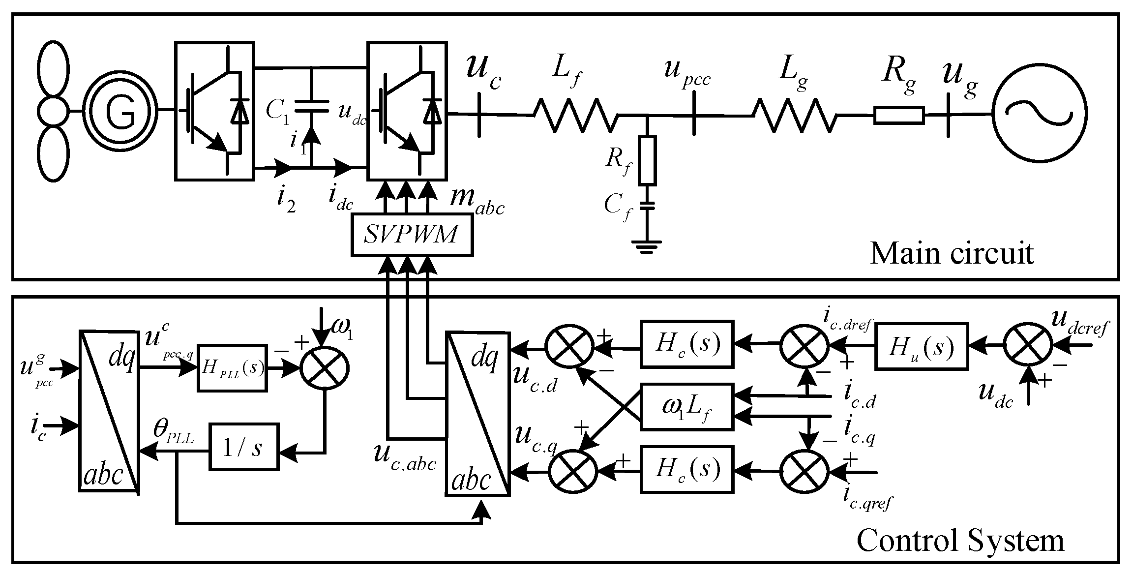
PMSGs primarily consist of a permanent magnet synchronous machine, machine-side converter, grid-side converter, and phase-locked loop, with the grid-connection topology shown in Figure 1. Due to the large capacitive energy storage capacity of the DC bus, dynamic coupling between the machine side and grid side can be isolated. During frequency regulation, the generator-side converter primarily extracts kinetic energy by adjusting rotor speed, while the grid-side converter manages grid-connected power control. Moreover, the generator-side dynamic time constant significantly exceeds both the grid-side dynamic time constant and the stability analysis frequency range. Consequently, the generator-side dynamics have negligible impact on the high-frequency stability of the grid-connected system. Therefore, modeling the generator side as an equivalent constant power source simplifies the model without compromising core stability-related information.

2.1.1. Small-Signal Model of the PLL

First, establish the small-signal model of the PLL. When subjected to small disturbances, the PLL generates corresponding disturbance components, causing phase differences between the control loop and the main circuit, which affects the equivalent impedance of the wind turbine. To distinguish between main circuit parameters and control loop parameters, this paper denotes components in the main circuit coordinate system with the superscript “g” and components in the coordinate system corresponding to the phase angle of the PLL output with the superscript “c”. The expression for the PLL output disturbance angle and the expression describing the difference relationship between the main circuit coordinate system and the control coordinate system caused by small disturbances affecting the grid connection point voltage are as follows:

$$\left\{\begin{array}{l}\Delta {\theta }_{PLL}={\displaystyle \frac{H_{PLL}(s)\Delta u_{pcc.q}^c}{s}}\\ \left[\begin{array}{l}\Delta u_{pcc.d}^c\\ \Delta u_{pcc.q}^c\end{array}\right]=\left[\begin{array}{l}\Delta u_{pcc.d}^g\\ \Delta u_{pcc.q}^g\end{array}\right]+\left[\begin{array}{cc}{\overline{u}}_{pcc.q}^g& 0\\ 0& {\overline{u}}_{pcc.d}^g\end{array}\right]\left[\begin{array}{l}\Delta {\theta }_{PLL}\\ -\Delta {\theta }_{PLL}\end{array}\right]\end{array}\right.$$

(1)

where Δθ_PLL is the PLL output disturbance angle; H_PLL(s) is the PLL transfer function, $H_{PLL}(s)=k_{PLL.p}+{\displaystyle \frac{k_{PLL.i}}{s}}$; Δu^c_pcc.q is the q-axis component of the grid-connection point voltage; s denotes d/dt; k_PLL.p and k_PLL.i are the proportional and integral control parameters of the PLL controller, respectively; Δu^c_pcc.d and Δu^c_pcc.q denote the disturbance components of the grid-connection point voltage along the axes in the phase-locked loop coordinate system; and ${\overline{u}}_{pcc.d}^g$, ${\overline{u}}_{pcc.q}^g$ Δu^g_pcc.d and Δu^g_pcc.q denote the steady-state and disturbance components of the grid-connection point voltage along the dq axes in the main circuit coordinate system.

The output voltage and current of the grid-side converter are influenced by the phase-locked loop. The correspondence between small-signal components in different coordinate systems can be derived and expressed as:

$$\left\{\begin{array}{l}\Delta u_{c.dq}^c=\Delta u_{c.dq}^g+G_{PLL.u}\Delta u_{pcc.dq}^g\\ \Delta i_{c.dq}^c=\Delta i_{c.dq}^g+G_{PLL.i}\Delta u_{pcc.dq}^g\end{array}\right.$$

(2)

Among them

$$G_{PLL.u}=\left[\begin{array}{cc}0& {\displaystyle \frac{H_{PLL}(s)}{s+H_{PLL}(s){\overline{u}}_{pcc.d}^g}}{\overline{u}}_{c.q}^g\\ 0& -{\displaystyle \frac{H_{PLL}(s)}{s+H_{PLL}(s){\overline{u}}_{pcc.d}^g}}{\overline{u}}_{c.d}^g\end{array}\right], G_{PLL.i}=\left[\begin{array}{cc}0& {\displaystyle \frac{H_{PLL}(s)}{s+H_{PLL}(s){\overline{u}}_{pcc.d}^g}}{\overline{i}}_{c.q}^g\\ 0& -{\displaystyle \frac{H_{PLL}(s)}{s+H_{PLL}(s){\overline{u}}_{pcc.d}^g}}{\overrightarrow{i}}_{c.d}^g\end{array}\right]$$

where Δu^c_c.dq, Δu^g_c.dq denote the disturbance components of the grid-side output voltage on the dq axes in the phase-locked loop coordinate system and the main circuit coordinate system, respectively; ${\overline{u}}_{c.dq}^g$, ${\overline{i}}_{c.dq}^g$ represent the dq-axis components of the grid-side output voltage and current in the main circuit, respectively; and G_PLL.u and G_PLL.i respectively denote the transfer functions of the grid-side output voltage and current to the grid-connection point voltage in different coordinate systems.

2.1.2. Small-Signal Model of the Current Inner Loop

To derive the small-signal model of the current inner loop, linearizing the dynamic equation of the wind turbine current control loop yields:

$$\left\{\begin{array}{l}\left[\begin{array}{l}\Delta u_{pcc.d}^g\\ \Delta u_{pcc.q}^g\end{array}\right]=\left[\begin{array}{l}\Delta u_{c.d}^g\\ \Delta u_{c.q}^g\end{array}\right]-G_l\left[\begin{array}{l}\Delta i_{c.d}^g\\ \Delta i_{c.q}^g\end{array}\right]\\ \left[\begin{array}{l}\Delta u_{c.d}^c\\ \Delta u_{c.q}^c\end{array}\right]=G_c\left[\begin{array}{l}\Delta i_{c.dref}\\ \Delta i_{c.qref}\end{array}\right]+\left(G_o-G_c\right)\left[\begin{array}{l}\Delta i_{c.d}^c\\ \Delta i_{c.q}^c\end{array}\right]\end{array}\right.$$

(3)

where $G_c=\left[\begin{array}{cc}{H}_c(s)& 0\\ 0& H_c(s)\end{array}\right]$ represents the inner-loop transfer function of the current; $H_c(s)=k_{cp}+{\displaystyle \frac{k_{ci}}{s}}$, $G_l=\left[\begin{array}{cc}s{L}_f& -{\omega }_1{L}_f\\ {\omega }_1{L}_f& s{L}_f\end{array}\right]$ is the transfer function of the filtering stage; $G_o=\left[\begin{array}{cc}0& {\omega }_1{L}_f\\ -{\omega }_1{L}_f& 0\end{array}\right]$ is the transfer function of the coupling impedance; L_f is the grid-side filtering inductor; ω₁ is the fundamental angular frequency. Substituting Equation (2) into Equation (3) yields:

$$\Delta u_{pcc.dq}^g={\displaystyle \frac{G_c\Delta i_{c.dqref}+(-G_c-G_l+G_o)\Delta i_{c.dq}^g}{\left(1-(G_o-G_c)G_{pll.i}+G_{pll.u}\right)}}$$

(4)

From the above equation, we can derive the relationship between Δu_pcc, Δi_c.ref and Δi_c for the PLL and the current inner loop.

2.1.3. Small-Signal Model of the Voltage Outer Loop Considering Power Output Effects

The control structure of the voltage outer loop for the grid-side converter of the wind turbine yields the expression for its output current reference value as follows:

$$\Delta i_{cdqref}=G_{uw}\Delta u_{dc}$$

(5)

where Δi_cdqref represents the small-signal component of the dq-axis reference output current of the grid-side converter, $G_{uw}=\left[\begin{array}{cc}{H}_u(s)& 0\\ 0& H_u(s)\end{array}\right]$ characterizing the transfer function of the voltage outer loop, $H_u(s)=k_{up}+{\displaystyle \frac{k_{ui}}{s}}$ Δu_dc denotes the small-signal quantity of the DC-side voltage. Next, we derive the expression for Δu_dc. From the grid-connected topology diagram, the power at both ends of the DC link is obtained as:

$$\left\{\begin{array}{l}\Delta p_s=\Delta u_{dc}{\overline{i}}_{dc}+{\overline{u}}_{dc}\Delta i_{dc}\\ \Delta p_c={\displaystyle \frac{3(\Delta u_{c.d}^g{\overline{i}}_{c.d}^g+{\overline{u}}_{c.d}^g\Delta i_{c.d}^g+\Delta u_{c.q}^g{\overline{i}}_{c.q}^g+{\overline{u}}_{c.q}^g\Delta i_{c.q}^g)}{2}}\\ \Delta i_{dc}=-s{C}_1\Delta u_{dc}\end{array}\right.$$

(6)

where Δp_s represents the increment in machine-side output power; Δp_c represents the grid-side input power; C₁ denotes the large capacitance in the DC link; and Δi_dc represents the current in the DC link. Since DC bus losses are relatively small compared to the machine-side output power, they can generally be neglected. Omitting these losses simplifies the derivation process for the small-signal model of the DC bus voltage and avoids introducing complex loss-related parameters. Therefore, neglecting power transmission losses in the DC link (that is, Δp_s = Δp_c), the expression for Δu_dc can be derived from the above equation:

$$△u_{dc}={\displaystyle \frac{3(\Delta u_{c.d}^g{\overline{i}}_{c.d}^g+{\overline{u}}_{c.d}^g\Delta i_{c.d}^g+{\overline{u}}_{c.q}^g\Delta i_{c.q}^g+\Delta u_{c.q}^g{\overline{i}}_{c.q}^g)}{2({\overline{i}}_{dc}-s{C}_1{\overline{u}}_{dc})}}$$

(7)

Substituting Equation (7) into Equation (5) yields the relationship expression between Δi_c.dqref, Δu^g_c.dq and Δi^g_c.dq:

$$\left\{\begin{array}{l}\Delta i_{c.dqref}=G_{uw}{G}_w{G}_{vi}\Delta i_{c.dq}^g+G_{uw}{G}_w{G}_{vu}\Delta u_{c.dq}^g\\ G_{vi}=\left[\begin{array}{cc}{\overline{u}}_{c.d}^g& {\overline{u}}_{c.q}^g\\ 0& 0\end{array}\right],G_{vu}=\left[\begin{array}{cc}{\overline{i}}_{c.d}^g& {\overline{i}}_{c.q}^g\\ 0& 0\end{array}\right],G_w={\displaystyle \frac{3}{2\left(i_{dc}-s{C}_1{u}_{dc}\right)}}\end{array}\right.$$

(8)

where G_vu denotes the small-signal transfer function of the DC link voltage; G_w represents the factor characterizing the impact of output level on wind turbine impedance; and G_vi denotes the small-signal transfer function of the DC link current. The relationship between i_dc and P_w can be established from the DC link power equation; thus, G_w can be used to characterize the impact factor of output level on wind turbine impedance:

$$G_w={\displaystyle \frac{3{\overline{u}}_{dc}}{2P_w-2s{C}_1{\overline{u}}_{dc}}}$$

(9)

2.1.4. Small-Signal Model of Direct-Drive Wind Turbines

The small-signal models for the phase-locked loop, current loop, and voltage loop have been established in the preceding sections. Building upon these models, this section further constructs the small-signal model for a direct-drive wind generator. Substituting Equation (8) into Equation (4) yields the relationship between $\Delta u_{pcc.dq}^g$ and $\Delta i_{c.dq}^g$. Based on this, further derivation provides the ratio of voltage to current at the grid connection point, which represents the equivalent impedance of the direct-drive wind generator:

$$Z_{dq}={\displaystyle \frac{\Delta u_{pcc.dq}^g}{\Delta i_{c.dq}^g}}={\displaystyle \frac{G_c{G}_{uw}{G}_w{G}_{vi}+G_c{G}_{uw}{G}_w{G}_{vu}{G}_l-G_c-G_l+G_o}{1-(G_o-G_c)G_{pll.i}+G_{pll.u}-G_c{G}_{uw}{G}_w{G}_{vu}}}$$

(10)

As demonstrated above, the output level of wind turbines affects the magnitude of impedance Z_dq by altering G_w, thereby causing changes in the stability of the grid-connected system. Therefore, it is necessary to analyze the impact of different wind turbine output levels on the stability of the grid-connected system.

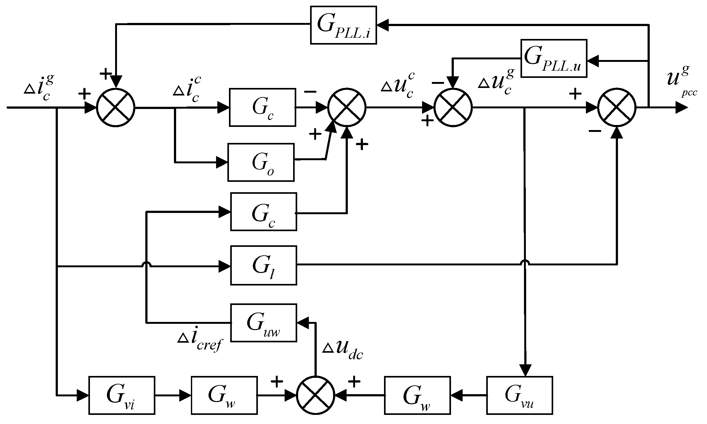
Figure 2 presents the small-signal control path diagram of the wind turbine, derived from the equivalent impedance model based on Equation (10) by integrating the transfer function matrices of the main circuit and each control loop. This equivalent impedance model is established in the synchronously rotating dq coordinate system, exhibiting inherent compatibility with the control system. However, the impedance model established in the dq coordinate system is a second-order impedance matrix that is difficult to measure directly. Stability analysis requires handling four elements and their coupling relationships simultaneously, making the analysis relatively complex. In contrast, the sequence impedance model possesses clear physical significance and straightforward stability criteria. For power systems operating normally with good symmetry, the primary determinant of stability is the positive-sequence impedance. Therefore, the derived dq impedance model is transformed into a positive-sequence impedance model for stability analysis. The conversion expression [23] is:

$$\left\{\begin{array}{l}{Z}_{PN}=\left[\begin{array}{cc}{Z}_{pp}& Z_{pn}\\ Z_{np}& Z_{nn}\end{array}\right]={\displaystyle \frac{1}{2}}\left[\begin{array}{cc}1& j\\ 1& -j\end{array}\right]Z_{dq}\left[\begin{array}{cc}1& 1\\ -j& j\end{array}\right]\\ Z_{PMSG}={\displaystyle \frac{\det (Z_{PN})}{Z_{nn}}}\end{array}\right.$$

(11)

where Z_PMSG represents the equivalent impedance of the wind turbine, denotes the sequence impedance, and Z_pp, Z_pn, Z_np, Z_pp respectively correspond to the four elements within the sequence impedance. det(.) denotes the matrix determinant. Through the transformation in Equation (11), the equivalent model is converted to the positive and negative sequence coordinate systems and reduced to the positive sequence impedance.

2.2. Grid-Connected Impedance Model for a Single Wind Turbine

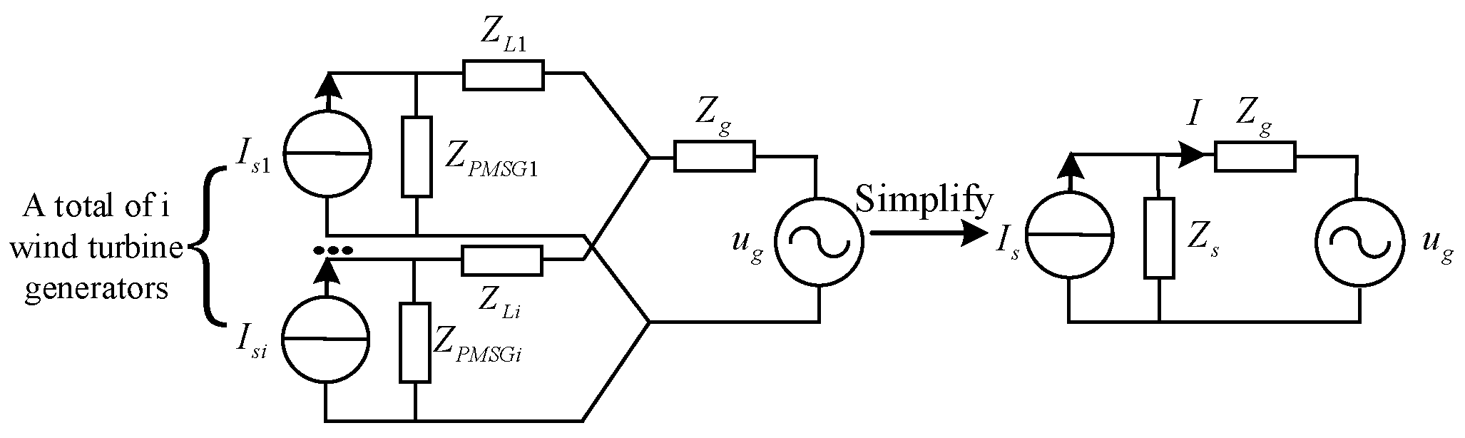
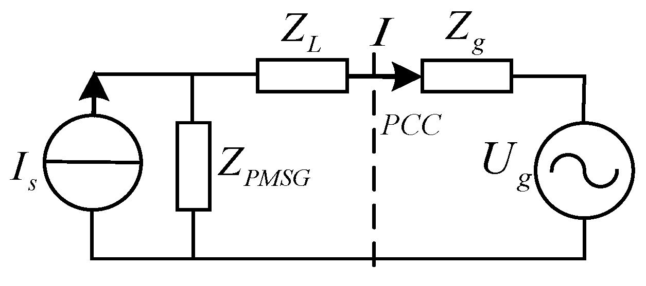
The previous subsection established the equivalent impedance of PMSG and its correlation with output power. This subsection further develops an impedance model for a single wind turbine connected to the grid. The PMSG is modeled as a constant current source with parallel equivalent impedance, connected to the grid via transmission lines, as shown in Figure 3.

From Figure 3, the output current I of the PCC is:

$$I={\displaystyle \frac{I_s{Z}_{PMSG}-U_g}{Z_{PMSG}+Z_L+Z_g}}={\displaystyle \frac{I_s-\frac{U_g}{Z_{PMSG}}}{1+\frac{Z_L+Z_g}{Z_{PMSG}}}}$$

(12)

The stability of a wind turbine grid-connected system is jointly determined by the equivalent impedance of the wind turbine, the line impedance, and the grid impedance. It can be assessed using the loop gain from Equation (12). In wind farm grid-connection systems, transmission lines typically consist of long medium-voltage cables. The reactance of such lines far exceeds their resistance, resulting in impedance dominated by reactance. Therefore, neglecting line resistance simplifies the terminal impedance model and aligns with the engineering reality of medium-to-long lines being reactance-dominated. If (Z_L + Z_g)/Z_PMSG satisfies the Nyquist criterion, the single direct-drive wind turbine grid-connected system can be considered stable. Therefore, mismatches between the output power of different wind turbines and the grid-connected line impedance may lead to reduced system stability or even instability.

2.3. Equivalent Impedance Model for Wind Farm Grid Connection

In actual wind farms, turbines connected to the same collection point may be located in different geographical areas and operate under varying conditions. Their power output levels differ, and their port impedances vary. Consequently, the power output of each turbine and its impedance matching with the port affect the stability of the grid-connected system. This section further establishes an equivalent impedance model for wind farm grid connection that accounts for active power output and terminal impedance. The simplification process of the equivalent impedance model for grid-connected systems is shown in Figure 4.

In the figure, I_s denotes the equivalent current source, Z_s represents the source-side impedance, and Z_gg indicates the grid-side equivalent impedance. Their respective expressions are:

$$\left\{\begin{array}{l}{I}_s=I_{s1}+I_{s2}+\dots +I_{si}\\ Z_s=Z_{PMSG1}\Vert Z_{PMSG2}\Vert \dots \Vert Z_{PMSGi}\\ Z_{gg}=\left(Z_{L1}\Vert Z_{L2}\Vert \dots \Vert Z_{Li}\right)+Z_g\end{array}\right.$$

(13)

Without considering inter-machine coupling, the current I of the PCC is:

$$I={\displaystyle \frac{{\displaystyle \sum _1^i{I}_{sn}}\left(Z_{PMSG1}\Vert \dots \Vert Z_{PMSGi}\right)-U_g}{\left(Z_{PMSG1}\Vert \dots \Vert Z_{PMSGi}\right)+\left(Z_{L1}\Vert \dots \Vert Z_{Li}\right)+Z_g}}={\displaystyle \frac{I_s{Z}_s-U_g}{Z_s+Z_{gg}}}={\displaystyle \frac{I_s-U_g/Z_s}{1+Z_{gg}/Z_s}}$$

(14)

Similarly, the stability of the wind farm grid-connected system is determined by the loop gain in Equation (14), which is defined by the impedance ratio between the grid side and the source side after each wind turbine is connected to the grid via transmission lines. If Z_gg/Z_s satisfies the Nyquist criterion, the wind farm grid-connected system can be considered stable.

3. Stability Analysis of Wind Farm Grid-Connected Systems

This section analyzes the stability of wind turbines at different physical locations under varying active power outputs based on the equivalent impedance model of the grid-connected wind farm.

3.1. Analysis of Active Power Output Variations

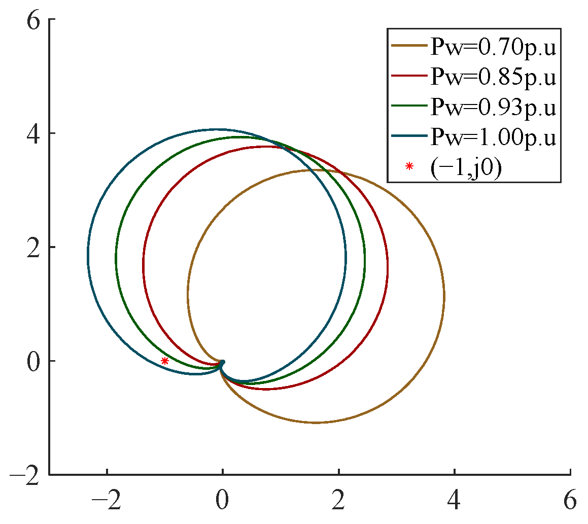
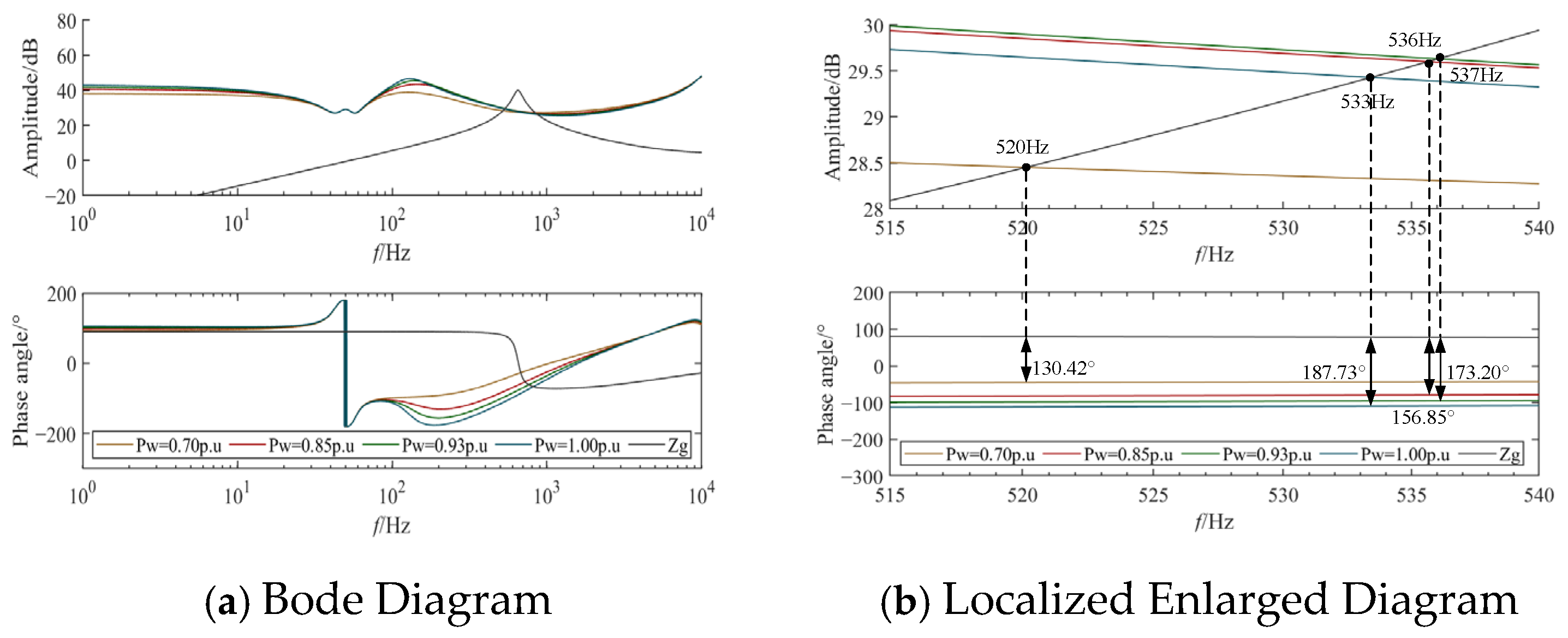
First, we examine the impact of turbine active power output on grid-connected system stability. Setting P_w to vary from 0.70 pu to 1.00 pu, the equivalent amplitude-frequency characteristic curve of the grid-connected system is shown in Figure 5. When P_w = 0.70 pu the magnitude curves of the wind turbine equivalent impedance and grid impedance intersect at 520 Hz with a phase angle difference of 130.42°, indicating system stability. When P_w = 0.85 pu the curves intersect at 536 Hz with a phase angle difference of 156.85°, resulting in a relatively reduced stability margin. When P_w further increases to 0.93 pu, the two magnitude curves intersect at 537 Hz with a phase angle difference of 173.2°, indicating a further reduction in the interconnection system’s stability margin. Finally, when P_w increases to 1.00 pu, the interconnection system becomes unstable. Figure 6 presents the impedance ratio Nyquist plot for the wind turbine grid-connected system as its active power output varies. It can be observed that as the active power output of the wind turbine increases, the Nyquist curve of the grid-connected system gradually approaches the point (−1, j0). According to the Nyquist criterion, when the active power output increases, the impedance ratio gradually approaches the point (−1, j0), and the stability margin becomes increasingly low.

Based on the above analysis, it can be seen that when the active power output changes from 0.70 pu to 1.00 pu, the stability of the interconnected system gradually weakens. This indicates that, with other wind turbine parameters remaining constant, the stability of the grid-connected system is significantly correlated with active power output: the higher the active power output, the weaker the stability of the grid-connected system. From the perspective of the entire grid-connected system, an increase in the active power output from the wind turbine corresponds to an increase in voltage drop across the grid impedance. This weakens the grid’s relative strength, consequently reducing system stability.

3.2. Analysis of Port Impedance Variations in Wind Turbines

Due to differing transmission line lengths from individual wind turbines to the collection point within a wind farm, variations in port impedance arise. For long lines, reactance significantly exceeds resistance. Consequently, the impact of line resistance on grid stability is negligible, necessitating analysis solely of how reactance variations affect stability.

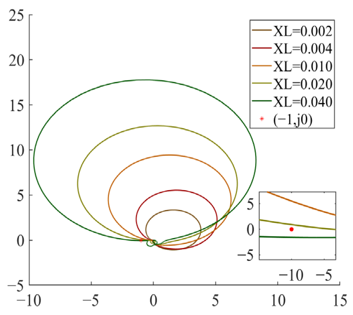
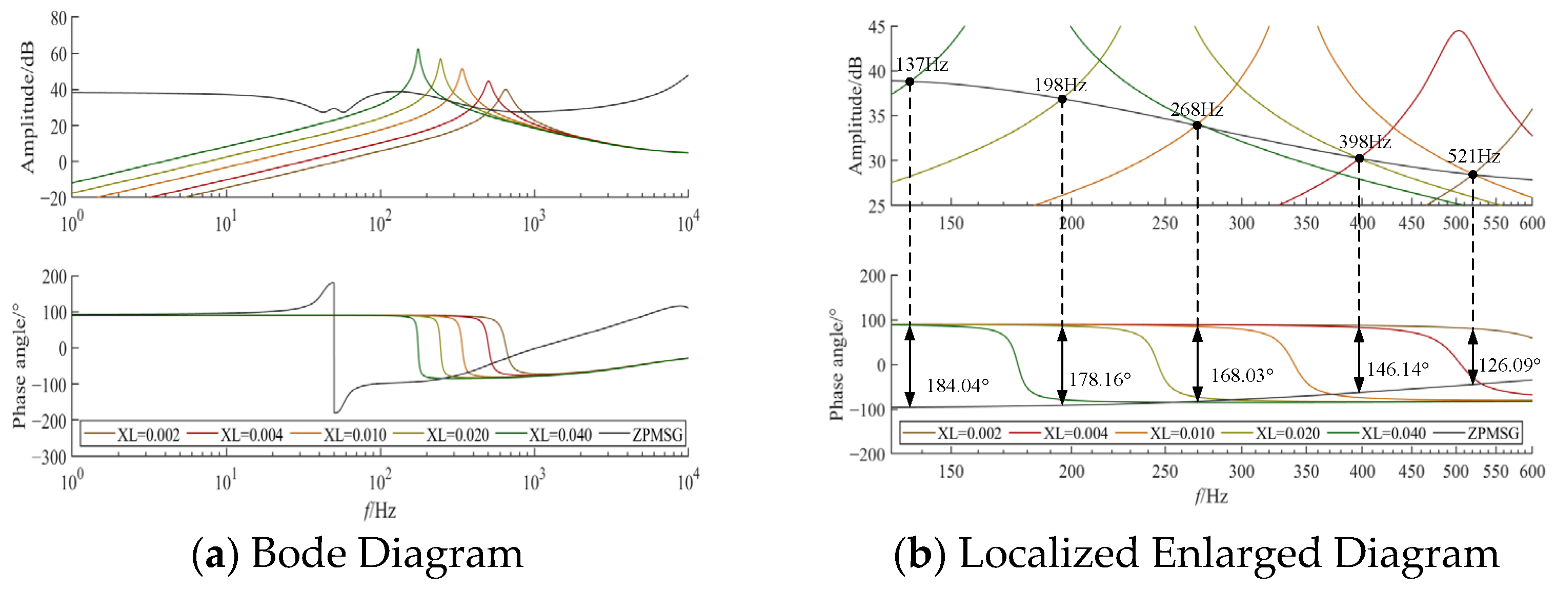
Setting the transmission line reactance to increase incrementally from 0.002 to 0.04, the change in the magnitude-frequency characteristics of the grid-connected system’s equivalent impedance is shown in Figure 7. When X_L = 0.002, the equivalent impedance of the wind turbine intersects the grid impedance magnitude curve at 521 Hz, with a phase angle difference of 126.09°, indicating a stable interconnection system. As X_L increases to 0.004, the impedance intersection frequency drops to 398 Hz, the phase angle difference increases to 146.14°, and the system stability margin decreases. When X_L further increases to 0.01, the intersection frequency decreases further to 268 Hz, the phase angle difference reaches 168.03°, and the margin decreases further. At X_L = 0.02, the phase angle difference at the intersection frequency of 198 Hz was 178.16°, bringing the system close to instability. Finally, at X_L = 0.04, the phase angle difference at the impedance intersection frequency of 134 Hz reached 184.04°, causing the interconnected system to become unstable. Figure 8 shows the impedance ratio Nyquist plot of the system as the impedance of the wind turbine grid-connected line varies. As the transmission line length increases, the Nyquist curve of the grid-connected system gradually approaches the point (−1, j0), reducing the stability margin. When X_L is set to 0.040, the curve encloses the point (−1, j0), causing the grid-connected system to become unstable.

Analysis of the phase angle margin and Nyquist criterion indicates that as X_L varies from 0.002 to 0.040, the stability of the interconnected system progressively deteriorates. This demonstrates that in direct-drive wind turbine grid-connected systems, system stability exhibits a negative correlation with transmission line length. This occurs because increased reactance at the wind turbine terminals weakens the equivalent strength of the grid-connected system, thereby heightening the risk of system instability.

3.3. Analysis of the Impact of Wind Turbine Port Impedance on Active Power Output Matching

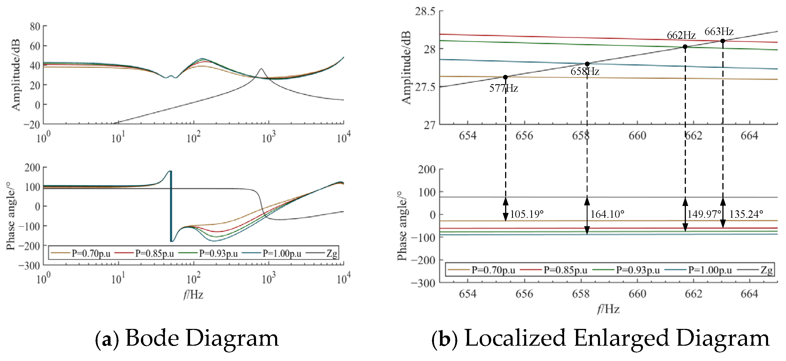
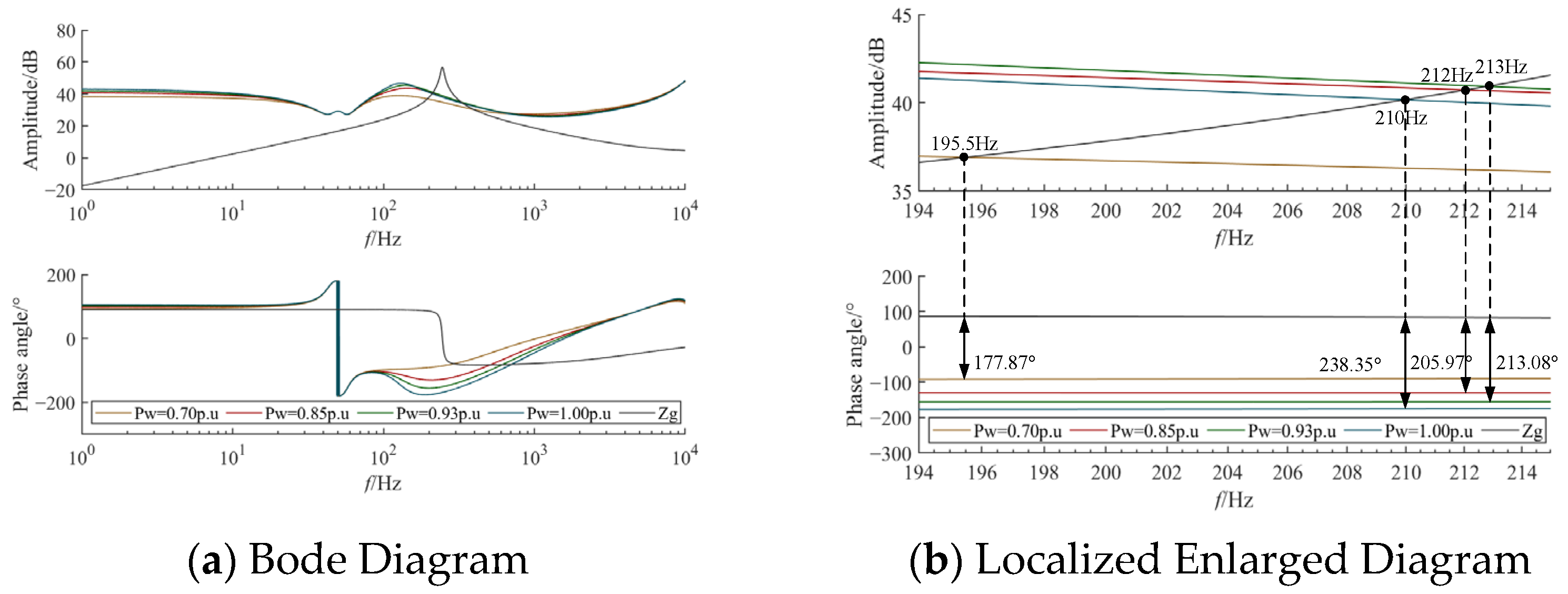
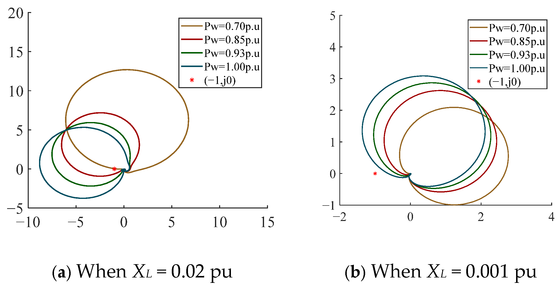
To examine system stability under varying active power outputs for wind turbines located at different physical positions, two typical scenarios were established: One with relatively high grid connection line impedance (X_L = 0.02 pu) and another with relatively low grid connection line impedance (X_L = 0.001 pu). The wind turbine output P_w was incrementally increased from 0.70 pu to 1.00 pu. The evolution patterns of the equivalent impedance magnitude-frequency characteristics and Nyquist traces were compared. The Bode plots of the grid-connected system are shown in Figure 9 and Figure 10, while the Nyquist plots are presented in Figure 11 and Figure 12.

As shown in Figure 9 and Figure 10, the magnitude-frequency curves of the equivalent impedance for grid-connected wind turbine systems at different physical locations reveal that as active power output increases, the phase angle difference significantly widens, reducing the system stability margin. The Nyquist plot in Figure 11a further validates this trend: increasing P_w causes the curve to progressively approach and eventually enclose the point (−1, j0), indicating a decline in grid-connected system stability. Simultaneously, when the grid-connected line impedance is high (X_L = 0.02 pu), the phase angle difference reaches 177.87° at P_w = 0.85 pu. Further increasing P_w to 1.00 pu causes the phase angle difference to exceed the 180° critical threshold, leading to instability. In contrast, under low grid connection line impedance (X_L = 0.001 pu), the grid connection system exhibits higher stability margins under identical active power output increases. Even when P_w increases to 1.00 pu, the phase angle difference rises to 164.10°, yet remains below the 180° critical threshold, maintaining system stability throughout. Corresponding to the Nyquist plot in Figure 11b, although the trajectory gradually approaches the point (−1, j0) as P_w increases, it still satisfies the Nyquist criterion’s non-envelopment condition. This demonstrates that when the grid-connected line impedance of wind turbines is high, smaller active power output should be matched to ensure grid stability. Conversely, when the grid-connected line impedance is low, wind turbines can match larger active power output while maintaining grid stability. For the overall grid-connected system of a wind farm, when the impedance of each wind turbine’s grid-connected line is highly matched with its active power output, the system’s stability margin increases. Conversely, when the matching degree is low, the system’s stability deteriorates.

Furthermore, taking two wind turbines with different distances to the collection point as examples, the wind farm controller responds to frequency regulation commands by allocating active power. This analysis compares how the matching degree between each turbine’s output and port impedance affects system stability. Here, the transmission line impedance X_L1 from Turbine A to the collection point is set to 0.001, while X_L2 from Turbine B is set to 0.20. With identical basic parameters for both turbines, the stability of the following three scenarios is analyzed:

• Scenario 1: Active power output allocated according to rated capacity;
• Scenario 2: Turbine A output 1.0 pu, Turbine B output 1.2 pu;
• Scenario 3: Turbine A output 1.2 pu, Turbine B output 1.0 pu.

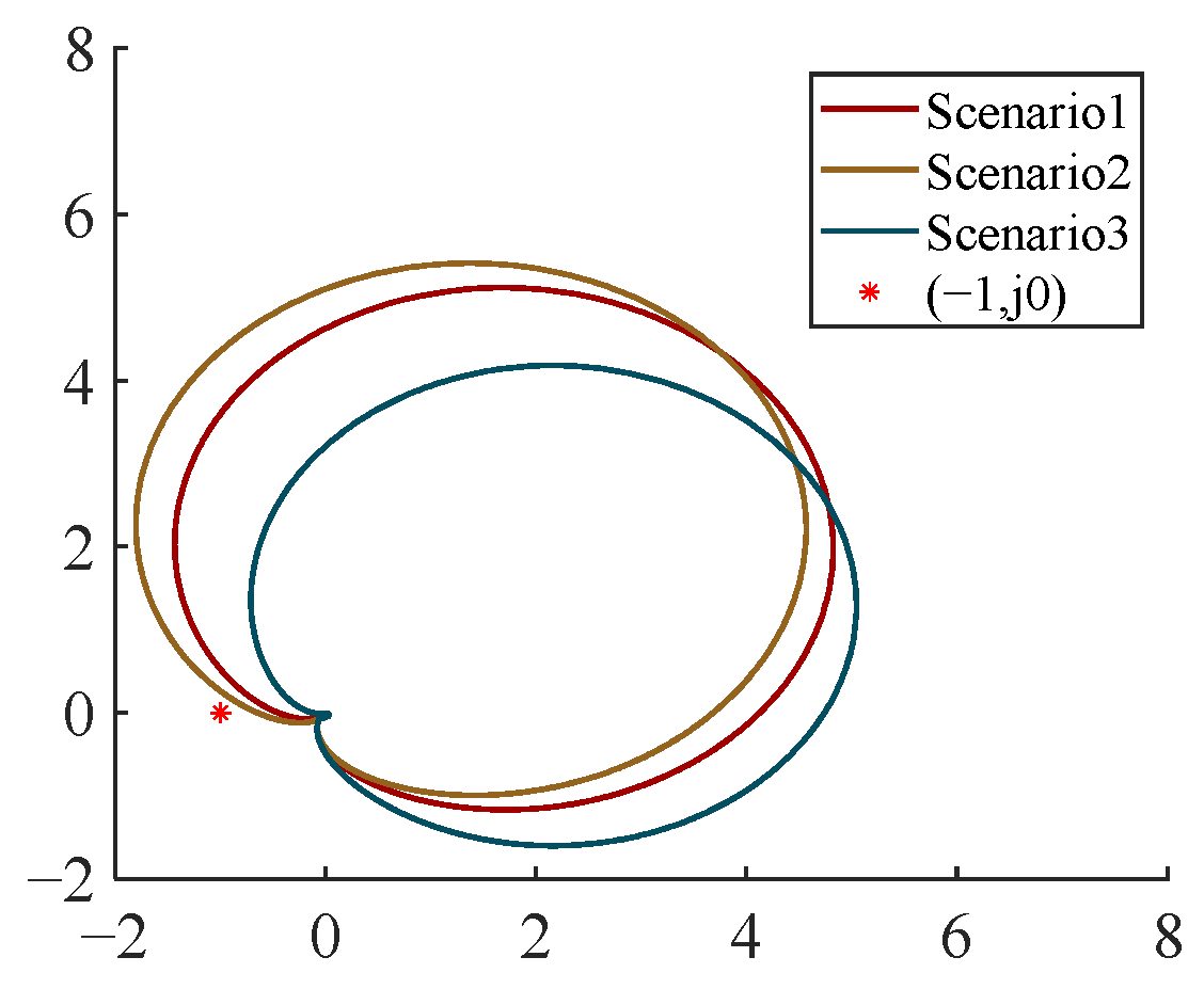
The system Bode plots for different scenarios are shown in Figure 12, Figure 13 and Figure 14, while the Nyquist curve comparisons for each scenario are illustrated in Figure 15.

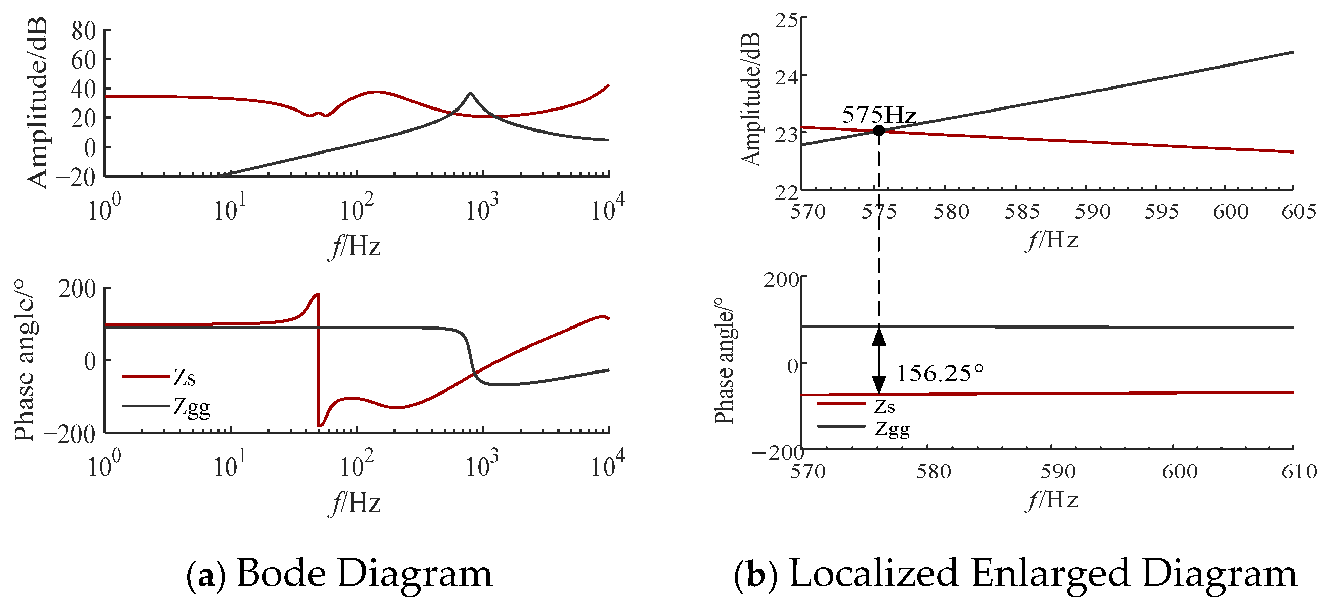
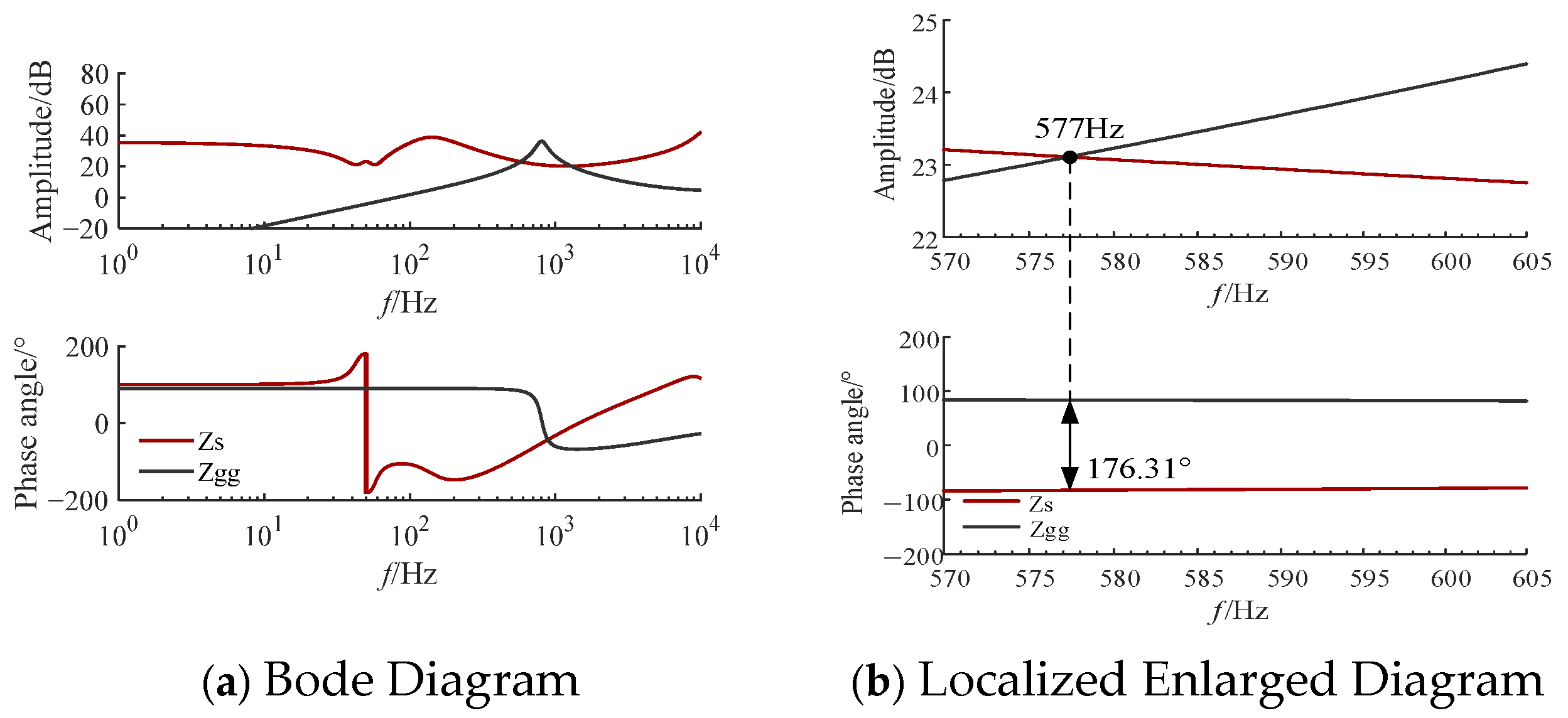
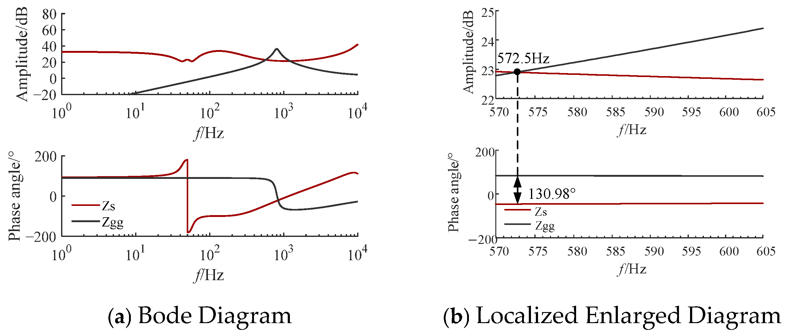
In Scenario 1, the impedance magnitude curves of the wind farm and power grid intersect at 575 Hz with a phase angle difference of 156.25°, indicating system stability. The yellow solid Nyquist trace representing Scenario 1 in Figure 15 does not enclose the point (−1, j0), verifying system stability. In Scenario 2, the intersection frequency slightly increases to 577 Hz, but the phase angle difference widens to 176.31°, resulting in a reduced stability margin compared to Scenario 1. The blue solid line in Figure 15 represents Scenario 2, where the Nyquist trace approaches the point (−1, j0). Although it does not enclose the critical point, the margin is relatively small. In Scenario 3, the intersection frequency of the two impedance magnitude curves is 572.5 Hz with a phase angle difference of 130.98°, representing a 106% increase in margin compared to Scenario 1. The red solid line in Figure 15, representing Scenario 3, shows a Nyquist trace far from the point (−1, j0), indicating system stability. Compared to the previous scenarios, this scenario offers a larger stability margin, better supporting system stability. In comparison, Wind Turbine A in Scenario 3, with its smaller grid-connected line impedance, shoulders a greater share of frequency regulation power. The matching degree between the turbine’s active power output and the port impedance is higher than in the other scenarios. Therefore, optimizing the allocation of active power for frequency regulation can significantly enhance the stability margin of the wind farm grid-connected system.

4. Optimized Frequency Regulation Power Allocation Strategy for Wind Farms Considering Stability Enhancement

4.1. Stability Margin Metrics for Wind Farm Grid-Connected Systems

This section proposes an optimization strategy for allocating active power frequency regulation among wind turbines within a wind farm to enhance stability. As analyzed in Section 2.3, the wind turbine grid-connected system can be modeled as an interaction between the source side and the grid. The stability of the grid-connected system is determined by Z_gg/Z_s, where the expressions for the equivalent grid-side impedance Z_gg and equivalent source-side impedance Z_s are respectively:

$$\left\{\begin{array}{l}{Z}_s=Z_{PMSG1}\Vert Z_{PMSG2}\Vert \dots \Vert Z_{PMSGi}\\ Z_{\mathrm{gg}}=\left(Z_{L1}\Vert Z_{L2}\Vert \dots \Vert Z_{Li}\right)+Z_g\end{array}\right.$$

(15)

From Equation (10), it can be seen that the active power output of each wind turbine affects its equivalent impedance, which in turn influences the equivalent source-side impedance Z_s of the wind farm in Equation (15). Meanwhile, the impedance of each wind turbine’s grid-connected line affects the equivalent grid-side impedance Z_gg. Therefore, the stability margin of the grid-connected system can be enhanced by optimizing the matching degree between the active power output of each wind turbine and the line impedance. The total impedance matrix Z_WF of the wind farm grid-connected system is defined as:

$$Z_{WF}=Z_s+Z_{\mathrm{gg}}=Z_{PMSG1}\Vert Z_{PMSG2}\Vert \dots \Vert Z_{PMSGi}+\left(Z_{L1}\Vert Z_{L2}\Vert \dots \Vert Z_{Li}\right)+Z_g$$

(16)

The stability margin of wind power grid-connected systems can be quantified and characterized by the damping ratio. For the impedance model of the wind farm grid-connected system shown in Equation (16), the set of eigenvalues is obtained from the characteristic equation, which is given by:

$$\det (Z_{WF})=\det \left(Z_{PMSG1}\Vert \dots \Vert Z_{PMSGi}\right.\left.+(Z_{L1}\Vert \dots \Vert Z_{Li})+Z_g\right)$$

(17)

Equation (17) yields the set of n eigenvalues for the grid-connected system, $\lambda =[{\lambda }_1,{\lambda }_2,\dots {\lambda }_n]=[{\sigma }_1+j{\omega }_1,{\sigma }_2+j{\omega }_2,\dots ,{\sigma }_n+j{\omega }_n]$, where σ_i and ω_i represent the real and imaginary parts of the i-th eigenvalue, respectively. For stable systems (i.e., where the real part of eigenvalues is less than zero), the damping ratio ξ reflects the rate at which transient oscillations in the system decay. The larger ξ is, the faster the oscillations decay. There exists a dominant eigenvalue ξ, corresponding to the eigenvalue with the largest real part and closest to the imaginary axis; that is to say $\widehat{\lambda }=\widehat{\sigma }+j\widehat{\omega }$ and $\mathrm{Re}(\widehat{\lambda })=\widehat{\sigma }=-\min (|{\sigma }_1|,|{\sigma }_2|,\dots ,|{\sigma }_n|)$, which has the most significant impact on the stability of grid-connected systems. At this point, the damping ratio corresponding to the dominant eigenvalue $\widehat{\zeta }$ is

$$\widehat{\zeta }=-{\displaystyle \frac{\widehat{\sigma }}{\sqrt{{\widehat{\sigma }}^2+{\widehat{\omega }}^2}}}={\displaystyle \frac{\min (|{\sigma }_1|,|{\sigma }_2|,\dots ,|{\sigma }_n|)}{|\widehat{\lambda }|}}$$

(18)

where $\widehat{\zeta }$ represents the damping ratio corresponding to the dominant eigen value $\widehat{\lambda }$, while $\widehat{\sigma }$ and $\widehat{\omega }$ denote the real and imaginary parts of the dominant eigenvalue, respectively. The system becomes more stable as σ < 0 and $\widehat{\zeta }$ increases. Therefore, this section sets the stability margin indicator for wind farm grid-connected systems as:

$$\delta \%={\displaystyle \frac{\widehat{\zeta }-{\zeta }_{\lim }}{\widehat{\zeta }}}={\displaystyle \frac{\frac{\min (|{\sigma }_1|,|{\sigma }_2|,\dots ,|{\sigma }_n|)}{|\widehat{\lambda }|}-{\zeta }_{\lim }}{\frac{\min (|{\sigma }_1|,|{\sigma }_2|,\dots ,|{\sigma }_n|)}{|\widehat{\lambda }|}}}$$

(19)

where $\widehat{\zeta }$ is the damping ratio corresponding to the dominant characteristic value of the current grid-connected system and ${\zeta }_{\lim }$ is the critical stability damping ratio of the grid-connected system. According to China’s national engineering standards, the damping ratio of power system oscillation modes should be greater than or equal to 0.05 to prevent sustained oscillations. Therefore, setting ${\zeta }_{\lim }$ = 0.05 ensures stable system operation under both normal and weak grid conditions.

4.2. Multi-Turbine Frequency Regulation Power Optimization Model Considering Stability Enhancement

This section constructs a mathematical model for optimizing frequency regulation power allocation in grid-connected wind farms with stability enhancement. The objective function maximizes the damping ratio of the grid-connected wind farm system while incorporating stability constraints, power balance constraints, and active power output constraints of individual turbines. While ensuring the grid-connected wind turbine system meets system frequency regulation power demands and stability requirements, the model enhances stability margin by maximizing the damping ratio. To satisfy stability constraints, the phase margin must exceed 0°, and the amplitude margin must exceed 0 dB. The frequency regulation power optimization allocation model for wind farms is as follows:

$$\begin{array}{l}\max \delta \%\\ s.t.\left\{\begin{array}{l}\gamma ={180}^{\circ }+\arg Z_s-\arg Z_{gg}>0\\ h=-20\lg \left|{\displaystyle \frac{Z_{gg}}{Z_s}}\right|>0\\ P_L={\displaystyle \sum _{k=1}^n{P}_{wk},\hspace{0.33em}{P}_{wk\min }\le P_{wk}\le P_{wk\max }}\end{array}\right.\end{array}$$

(20)

In the optimization model, the grid-connected system must satisfy the inequality constraints for phase margin and amplitude margin during stable operation. The expression for the amplitude margin h of the grid-connected system is:

$$h=-20\lg \left|{\displaystyle \frac{Z_{gg}(j{\omega }_{\mathrm{g}})}{Z_{\mathrm{s}}(j{\omega }_{\mathrm{g}})}}\right|$$

(21)

where ω_g denotes the crossover frequency between the equivalent source-side output impedance Z_s and the equivalent grid impedance Z_gg.

Substituting further into Equation (15) yields:

$$\left\{\begin{array}{c}\gamma =180°+\arg \left[Z_{PMSG1}(j{\omega }_{\mathrm{c}})\Vert \dots \Vert Z_{PMSGi}(j{\omega }_{\mathrm{c}})\right]\\ -\arg \left[Z_{L1}(j{\omega }_{\mathrm{c}})\Vert \dots \Vert Z_{Li}(j{\omega }_{\mathrm{c}})+Z_g(j{\omega }_{\mathrm{c}})\right]\\ \\ h=-20\lg \left|{\displaystyle \frac{\left(Z_{L1}(j{\omega }_g)\Vert \dots \Vert Z_{Li}(j{\omega }_g)\right)+Z_g(j{\omega }_g)}{Z_{PMSG1}(j{\omega }_g)\Vert \dots \Vert Z_{PMSGi}(j{\omega }_g)}}\right|\end{array}\right.$$

(22)

where Z_PMSGi(jω_c) and Z_Li(jω_c) represent the equivalent impedance of the i-th wind turbine and the corresponding grid-connected line impedance at the intersection frequency, respectively. Z_PMSGi(jω_g) and Z_Li(jω_g) represent the equivalent impedance of the i-th wind turbine and the corresponding grid-connected line impedance at the ride-through frequency, respectively.

Simultaneously, during frequency regulation of the wind power grid-connected system, the following constraints must be satisfied: the equality constraint between the wind farm’s power adjustment quantity and the system’s frequency regulation power demand, as well as the upper and lower output limits for each wind turbine, i.e.,

$$\left\{\begin{array}{l}\Delta P={\displaystyle \sum _{k=1}^n{P}_{w\mathrm{k}}}\\ P_{wk\min }\le P_{wk}\le P_{wk\max }\end{array}\right.$$

(23)

where ΔP represents the system’s frequency modulation power demand, P_wk denotes the active power output of the kth wind turbine, while P_wkmin and P_wkmax denote the minimum and maximum active power outputs that each wind turbine can deliver, respectively. The maximum output is determined by the rated capacity of the wind turbine and the available wind speed, P_wkmax = min(P_N,0.5ρπC_pR²v³), where P_N is the rated capacity of the wind turbine and ρ = 1.225 kg/m³, R, and C_p are inherent parameters of the wind turbine. Minimum output is determined by the rotor’s minimum stable rotational speed and the converter’s operational limits. Therefore, the upper and lower output constraints for wind turbines can be determined by considering factors such as the available rotor kinetic energy and operating conditions like wind speed for each turbine [30,31,32].

PSO demonstrates significant advantages in computational complexity, objective function requirements, and parameter tuning difficulty when addressing frequency regulation power allocation in wind farms. Therefore, it is adopted as the optimization algorithm for the active power allocation scheme proposed in this paper. The key parameters of PSO are carefully tuned to balance convergence speed and optimization accuracy, considering the nonlinearity and multi-constraint characteristics of the model. Assuming the AC grid configuration is known, along with the known line lengths from each turbine to the PCC, and that the network topology and terminal impedances specified are known, the specific algorithmic steps for solving the frequency regulation power optimization configuration when the frequency regulation controller issues a regulation command to the wind farm’s central control system are as follows:

Step 1: Input the control parameters, port impedance, network structure parameters, and system frequency regulation power demand for each wind turbine in the grid-connected system;

Step 2: Employ the particle swarm optimization algorithm to initialize the frequency regulation active power configuration. Calculate the equivalent impedance model of the wind farm grid-connected system under this configuration, derive the corresponding system damping ratio, and compute the current damping ratio stability margin;

Step 3: Determine whether the grid-connected system meets the constraint conditions under this configuration. If satisfied, proceed to the next step; otherwise, return to Step 2.

Step 4: Record the stability margin calculated from the first set of constraint-satisfying configurations as the initial value. Compare the stability margin under the current configuration with the initial value. If the stability margin under the current configuration is greater, update the maximum value.

Step 5: Output the maximum stability margin and the corresponding optimized active power configuration for system frequency regulation.

4.3. Frequency Regulation Power Allocation Scheme

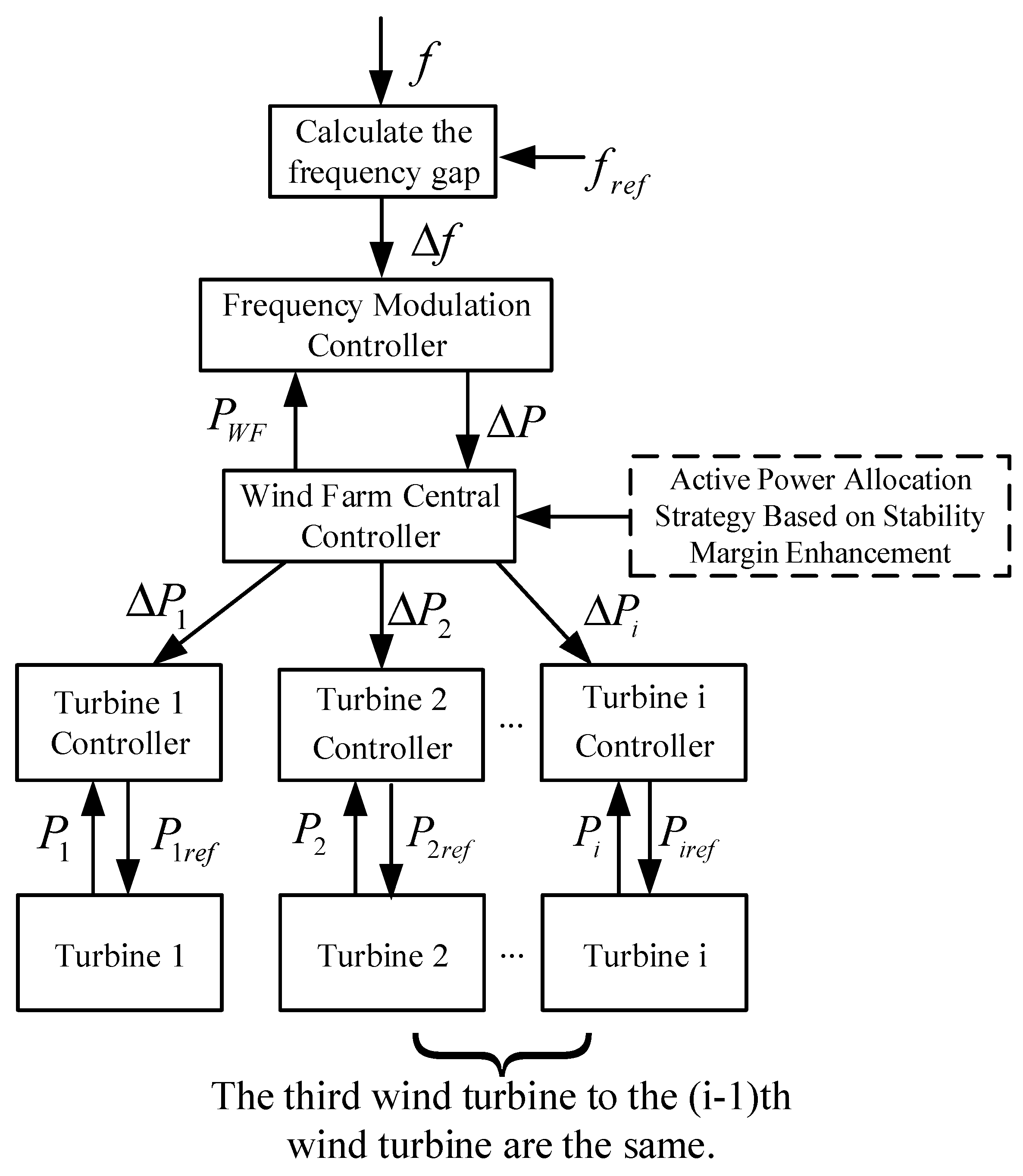
When a wind farm responds to frequency regulation demands, the dispatch center first calculates the total power adjustment required ΔP to meet primary frequency regulation requirements based on the received system frequency deficit Δf and the wind farm’s current total available output power P_WF. Upon receiving this ΔP command, the wind-farm-level central controller does not immediately distribute ΔP equally among all units. Instead, it executes an active power optimization allocation strategy based on stability margin enhancement. The core inputs for this strategy include the current maximum power output P_wi of each wind turbine within the farm and real-time assessments of the grid system’s stability margin. The optimization strategy calculates a specific power adjustment for each unit. This adjustment is superimposed onto the unit’s original power setpoint to generate a new active power target command P_wiref, which is then dispatched to the corresponding wind turbine. The core objective of this optimization scheme is to effectively enhance the grid stability margin of the entire wind farm while satisfying the frequency regulation command. A schematic illustration is shown in Figure 16.

5. Case Study Analysis

To validate the effectiveness of the proposed modeling and frequency-modulating power allocation scheme, this section conducts a case study analysis using the PSCAD/EMTDC simulation platform. A wind farm comprising a specific model of PMSG units serves as the example. The structural and control parameters of the PMSG are detailed in

Table 2. Wind Turbine Parameter Table.

Parameters	Value	Parameters	Value
DC link voltage	1100 V	Current Loop Proportional Constant	0.6
DC link capacitor	8 mF	Voltage Loop Proportional Constant	0.1
Current loop integral constant	200	PLL proportional constant	180
Voltage loop integral constant	15	Phase-locked loop integral constant	2000
Rated capacity of wind turbines	2 MW	Power grid frequency	60 Hz

.

5.1. Example 1

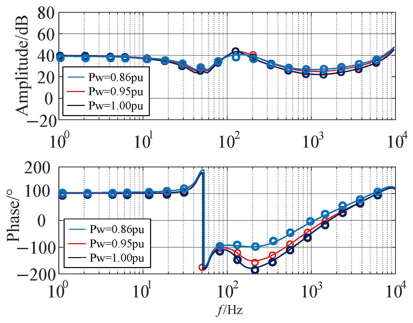
This section first employs the sweep method to validate the impedance model of the wind turbine grid-connected system constructed in Chapter 1. The grid-connected system parameters are listed in

Table 3. Parameter Table of Example 1.

Parameters	Value	Parameters	Value
Filter Inductor Lf	1 mH	Filter Capacitor Cf	20 uF
Filter Resistor Rf	0.001 Ω	Frequency	60 Hz
Equivalent Reactance of the Grid Lg	5 mH	Voltage of PCC upcc	35 kV
Grid Connection Line Impedance XL	2 mH	Equivalent Resistor of the Grid Rg	0.002 Ω

, and the simulation model of the grid-connected wind turbine is shown in Figure 1. A positive-sequence voltage disturbance signal is injected at the PCC. The wind turbine impedance model and positive-sequence sweep simulation results are presented in Figure 17. In the figure, solid lines represent the calculated values of the positive-sequence impedance model considering active power output, while “o” denotes the sweep results. Figure 17 shows that the calculated results of the impedance model exhibit minimal deviation from the sweep results. Changes in active power output significantly impact the stability of the wind power grid-connected system. As the wind turbine output increases, its phase characteristic curve approaches −180°, progressively weakening the stability of the grid-connected system. This validates the theoretical correctness and effectiveness of the equivalent impedance model.

5.2. Example 2

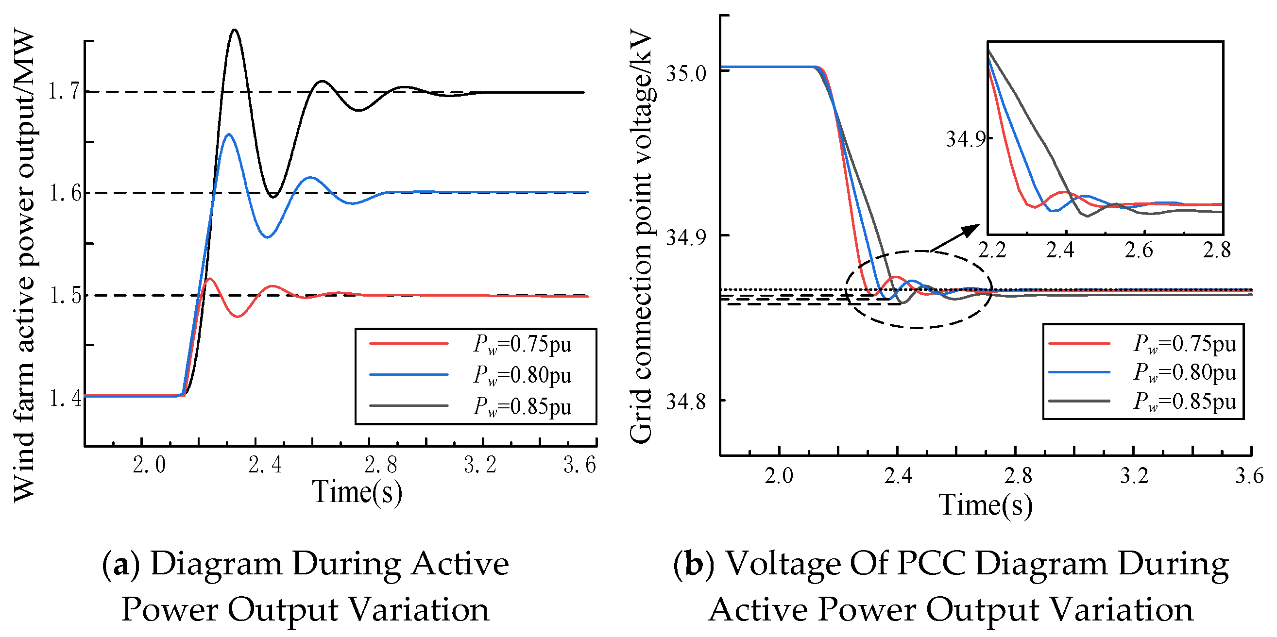
This section verifies the stability of the wind turbine grid-connected system shown in Figure 1 under the influence of active power and port impedance. Grid-connection parameters are detailed in

Table 4. Parameter Table of Example 2.

Parameters	Value	Parameters	Value
Wind Turbine Terminal Inductor	0.02 pu	Wind Turbine Terminal Resistance	0.005 pu
Equivalent Inductor of The Grid	0.01 pu	Equivalent Resistance of The Grid	0.001 pu

. The initial active power output of the wind farm is set to 0.7 pu. The grid-connected system reaches the initial stable operating point at 2.0 s. At 2.1 s, the active power output is increased to 0.75 pu, 0.80 pu, and 0.85 pu, respectively. The simulation waveforms are shown in Figure 18. As active power output increased, the transient processes of wind turbine output power and voltage of PCC changed. Overshoot gradually increased, oscillation duration lengthened, and the recovery time from disturbance onset to attenuation within permissible limits significantly increased. The system’s damping characteristics weakened, and stability margin continuously decreased. These results confirm the impact of active power output on grid-connection system stability, consistent with the conclusions drawn in Section 2’s frequency-domain amplitude analysis.

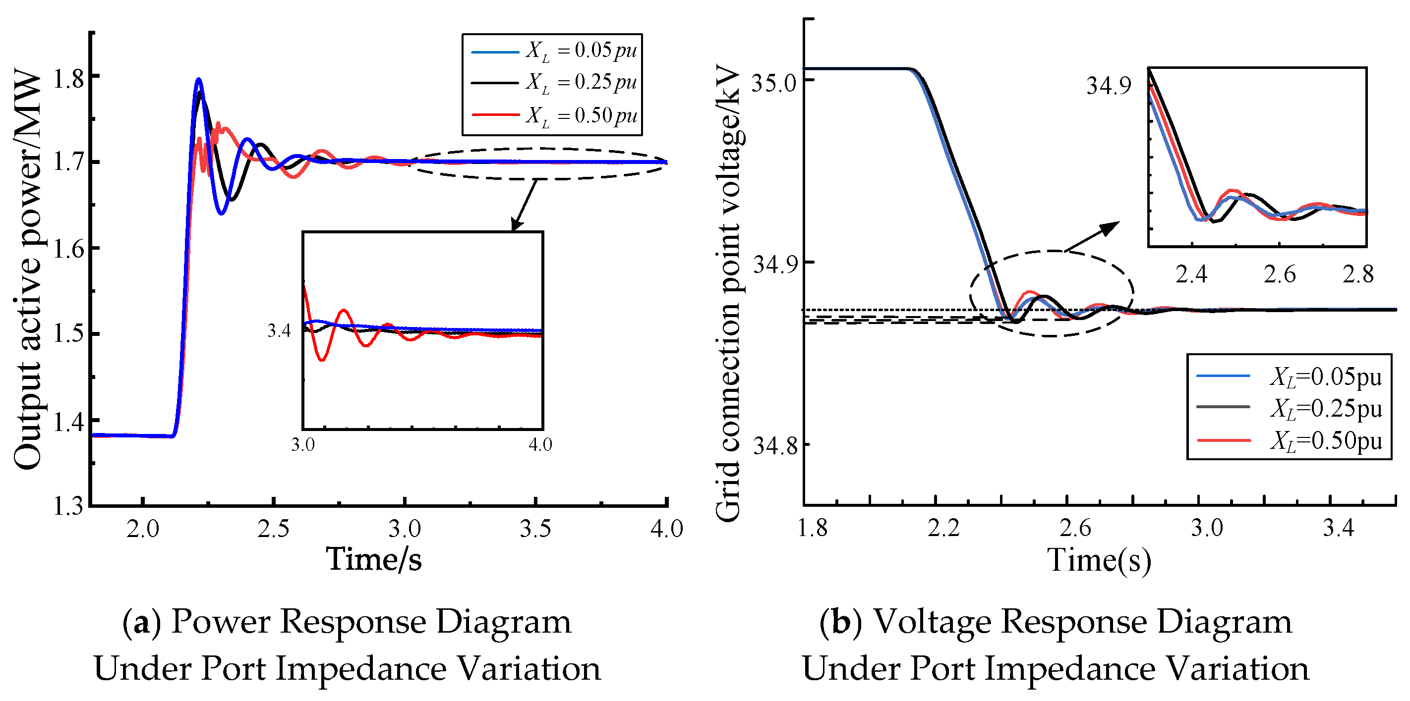
Further, the port reactance X_L was set to three values: 0.05 pu, 0.25 pu, and 0.5 pu, with all other parameters identical to those in Table 3. The initial active power output of the wind farm was set to 0.69 pu, and the system reached the initial steady-state operating point at 2.0 s. At 2.1 s, the active power output abruptly increased to 0.85 pu. The simulation waveforms are shown in Figure 19. As X_L increases, the disturbance response characteristics of the grid-connected system deteriorate. Oscillation amplitude increases, recovery time significantly lengthens, system damping weakens, and stability margin continuously decreases. These results indicate a negative correlation between port impedance and grid-connected system stability, consistent with the frequency-domain amplitude analysis conclusions in Section 2.

5.3. Example 3

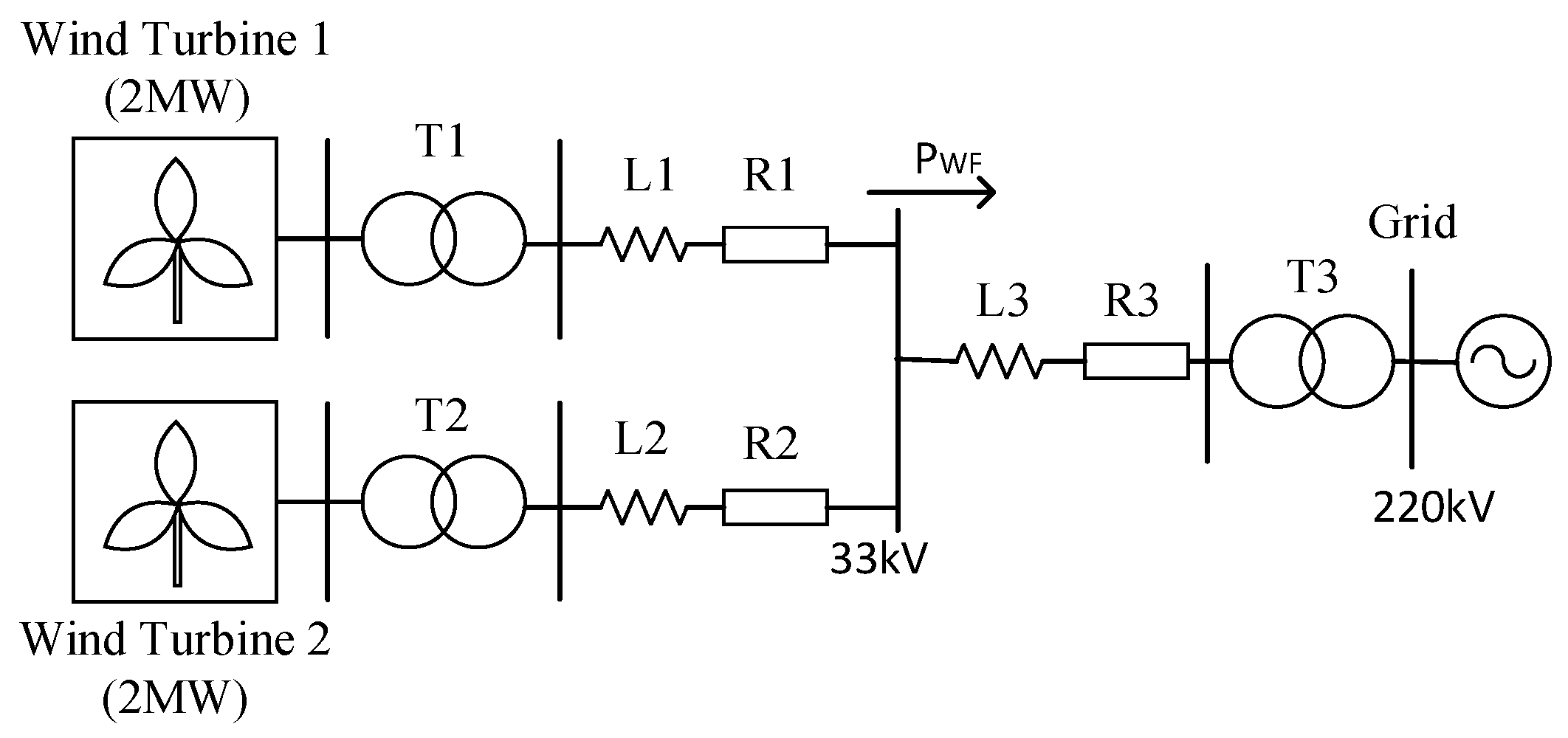
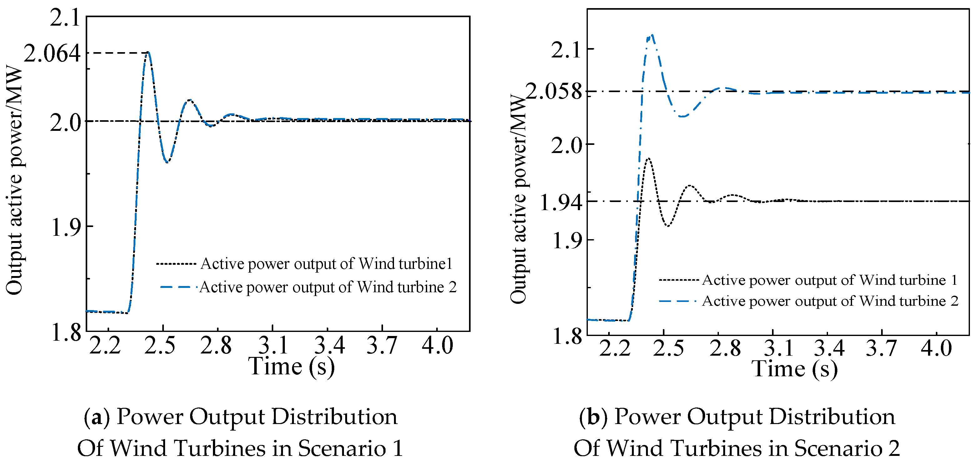
This subsection validates the effectiveness of the proposed frequency regulation power allocation optimization strategy for a two-turbine grid-connected system, as illustrated in Figure 20. PSO optimization parameters and grid connection parameters are shown in

Table 5. Parameter Table of Example 3.

Parameters	Value	Parameters	Value
Wind Turbine 2-1 Average Wind Speed	10.0 m/s	Terminating Resistor R2-1	0.005 pu
Wind Turbine 2-2 Average Wind Speed	10.5 m/s	Terminating Resistor R2-2	0.008 pu
Terminal Inductor L2-1	0.05 pu	Equivalent Inductance Of The Grid L2-3	0.01 pu
Terminal Inductor L2-2	0.08 pu	Equivalent Resistor Of The Grid R2-3	0.001 pu
Population size	50	Cognitive acceleration coefficient	2
Maximum number of iterations	100	Social acceleration coefficient	2
Upper Boundary Constraint	$P_{wk\max }$	Lower Boundary Constraints	$P_{wk\min }$

, with both turbines exhibiting differences in terminal impedance and preset wind speeds. The initial active power output of the wind turbines is set to 0.9 pu, and the grid-connected system enters a steady state after t = 2.0 s. At t = 2.1 s, the wind farm responds to the system frequency regulation command. The frequency regulation output of the two wind turbines is appropriately adjusted and optimized according to three schemes These three schemes allocate frequency regulation power according to different active power distribution approaches. Among these schemes, Scheme 1 operates at rated power output, proportionally distributing frequency regulation power based on each turbine’s rated capacity. Scheme 2 operates at available power output, allocating total frequency regulation active power according to preset wind speeds. Scheme 3 employs a wind farm active power allocation scheme that prioritizes stability enhancement.

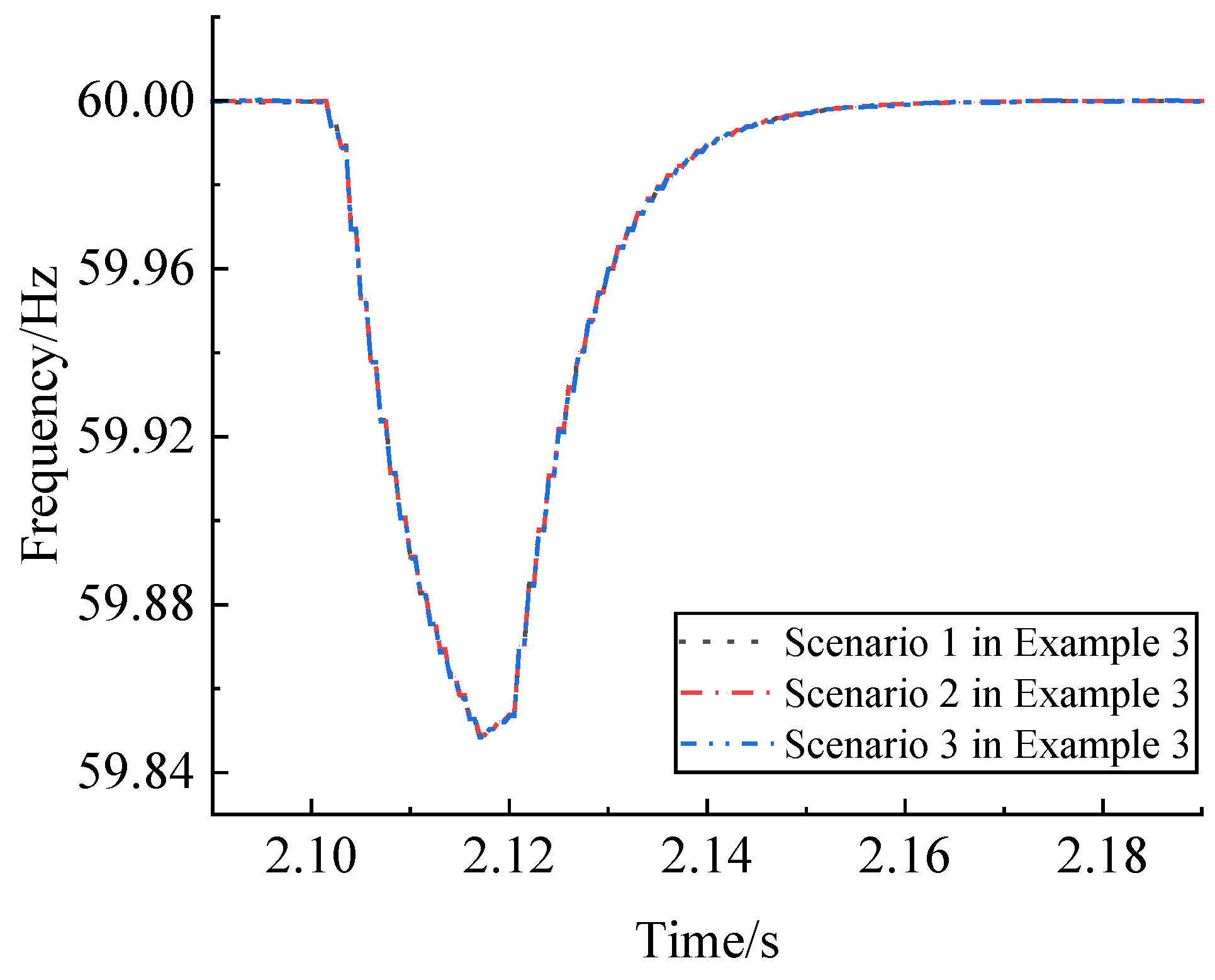
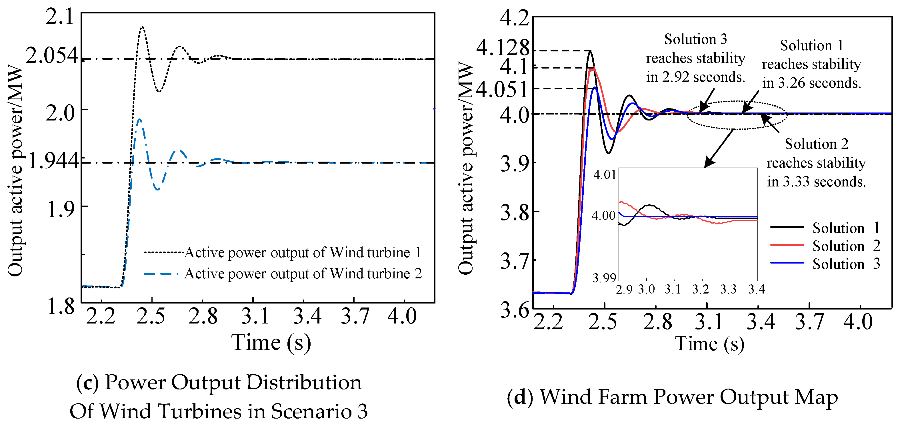
To validate the effectiveness of the proposed strategy, the wind farm responds to grid dispatch commands at t = 2.1 s, with active power output stepping from 0.9 pu to 1.0 pu. The time-domain simulation results for the system’s active power output under this scenario are shown in Figure 21d, while the frequency response diagram is presented in Figure 22.

Next, compare the impact of disturbances on system stability under different active power allocation schemes. As shown in the frequency response diagram, the frequency regulation performance is identical across all three schemes. This is because the frequency regulation power allocation strategy only affects power distribution between the two wind turbines, while the external active power output of the wind farm remains constant under all three approaches. As shown in Figure 21d, the system reaches steady-state operation before 2.0 s. Following the power disturbance at 2.1 s, the transient response processes of the three schemes exhibit significant differences. Under Scheme 1, which distributes disturbance power based on rated power, the wind farm’s active power output exhibits pronounced oscillations lasting 1.16 s, transitioning to a new steady state only at 3.26 s. Under Scheme 2, which distributes disturbance power based on available capacity, the oscillation amplitude is larger than in Scheme 1, with weaker damping and slower decay, extending the recovery time to 3.33 s; Scheme 3, employing the proposed allocation strategy, exhibits rapid oscillation decay, completing the transition in just 2.92 s, demonstrating the optimal stability performance among the three schemes.

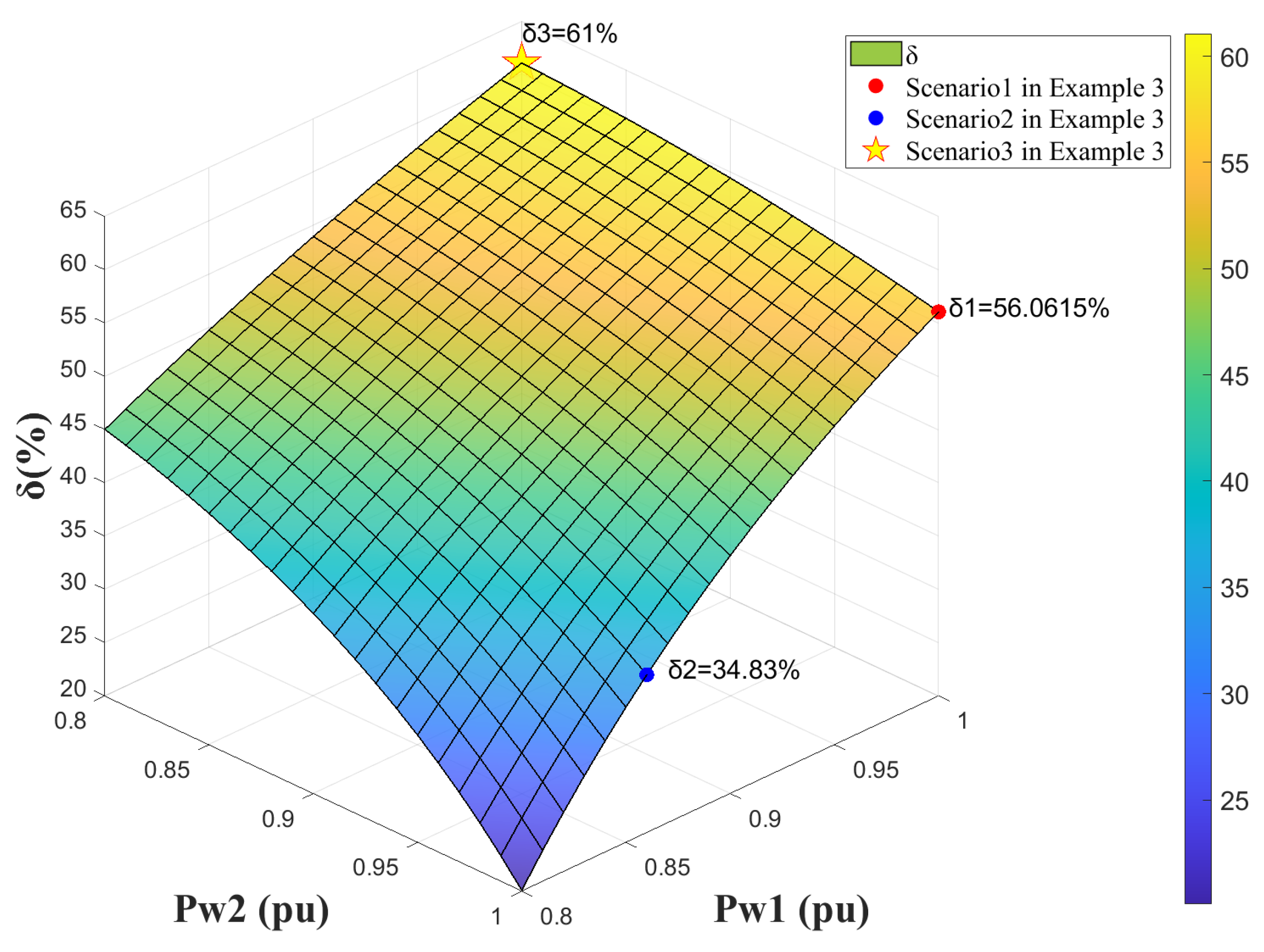
Figure 23 illustrates the damping ratio stability margin of the grid-connected system under different power allocation schemes. Scheme 1 and Scheme 2 exhibit margins of 56% and 34%, respectively. When applying the proposed allocation scheme, the damping ratio stability margin increases to 61%, validating the effectiveness of the proposed approach in enhancing system stability. Thus, Scheme 3 significantly improves grid-connected system stability by optimizing the matching between wind turbine active power output and port impedance. Under identical power disturbances, it exhibits the smallest overshoot, fastest oscillation decay, shortest recovery time, and higher stability margin compared to Scheme 1 and Scheme 2.

Table 6. Quantitative Comparison Table of Different Schemes in Example 3.

Performance Indicator	Equal Distribution	Capacity-Based Allocation	Proposed Strategy
Damping ratio stability margin	56%	34%	61%
Transient recovery time (s)	3.26	3.33	2.92
Active power overshoot (%)	3.2	2.5	1.3

shows the quantitative performance metric comparison for different approaches in Example 3.

5.4. Example 4

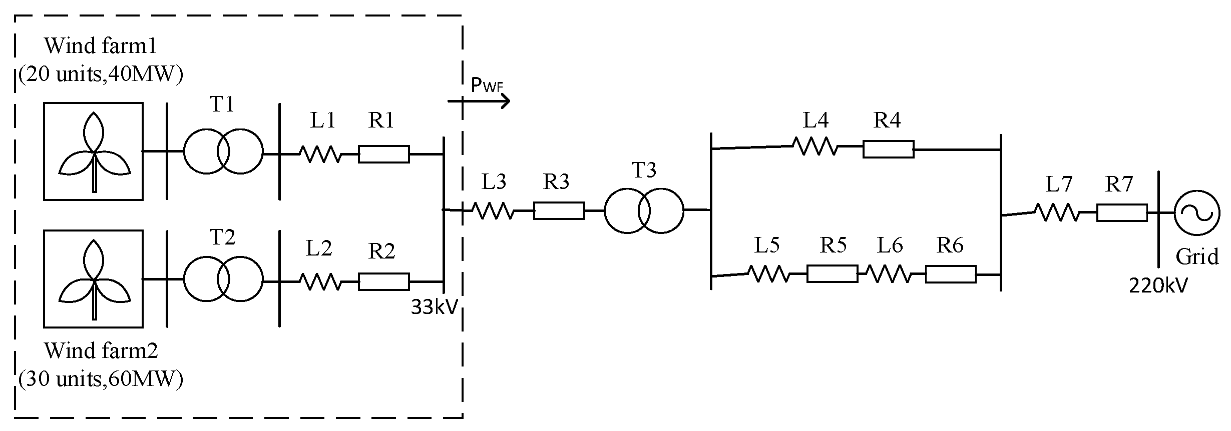
This section further validates the effectiveness and applicability of the analysis results and the proposed allocation scheme. A wind farm grid-connected system is constructed as shown in Figure 24, with system parameters and PSO optimization parameters listed in

Table 7. Parameter Table of Example 4.

Parameters	Value	Parameters	Value
Number of wind turbines in Wind Farm 1	25	R2-7	0.001
Number of wind turbines in Wind Farm 2	25	L2-1	0.05 pu
R2-1	0.005 pu	L2-2	0.08 pu
R2-2	0.008 pu	L2-3	0.2 pu
R2-3	0.02 pu	L2-4	0.3 pu
R2-4	0.03 pu	L2-5	0.15 pu
R2-5	0.015 pu	L2-6	0.15 pu
R2-6	0.015 pu	L2-7	0.01

. In Example 4, different numbers of wind turbines, on-site turbine parameters, turbine port impedances, and turbine operating conditions are considered. Wind Farm 1 and Wind Farm 2 are represented by equivalent turbines, characterizing the grid-connection parameters and operating states of the wind farms. The total initial active power output of the wind farms is set to 90% of the rated capacity. At 2.1 s, the system responds to the frequency regulation command issued by the dispatch center, increasing the total active power output to 100% of the rated capacity. Three power allocation schemes were employed to distribute frequency regulation power between Wind Farms 1 and 2: allocation based on rated active power, allocation based on available active power, and allocation based on the proposed scheme that considers stability enhancement. The active power output of the grid-connected system and the system frequency response are shown in the figure below.

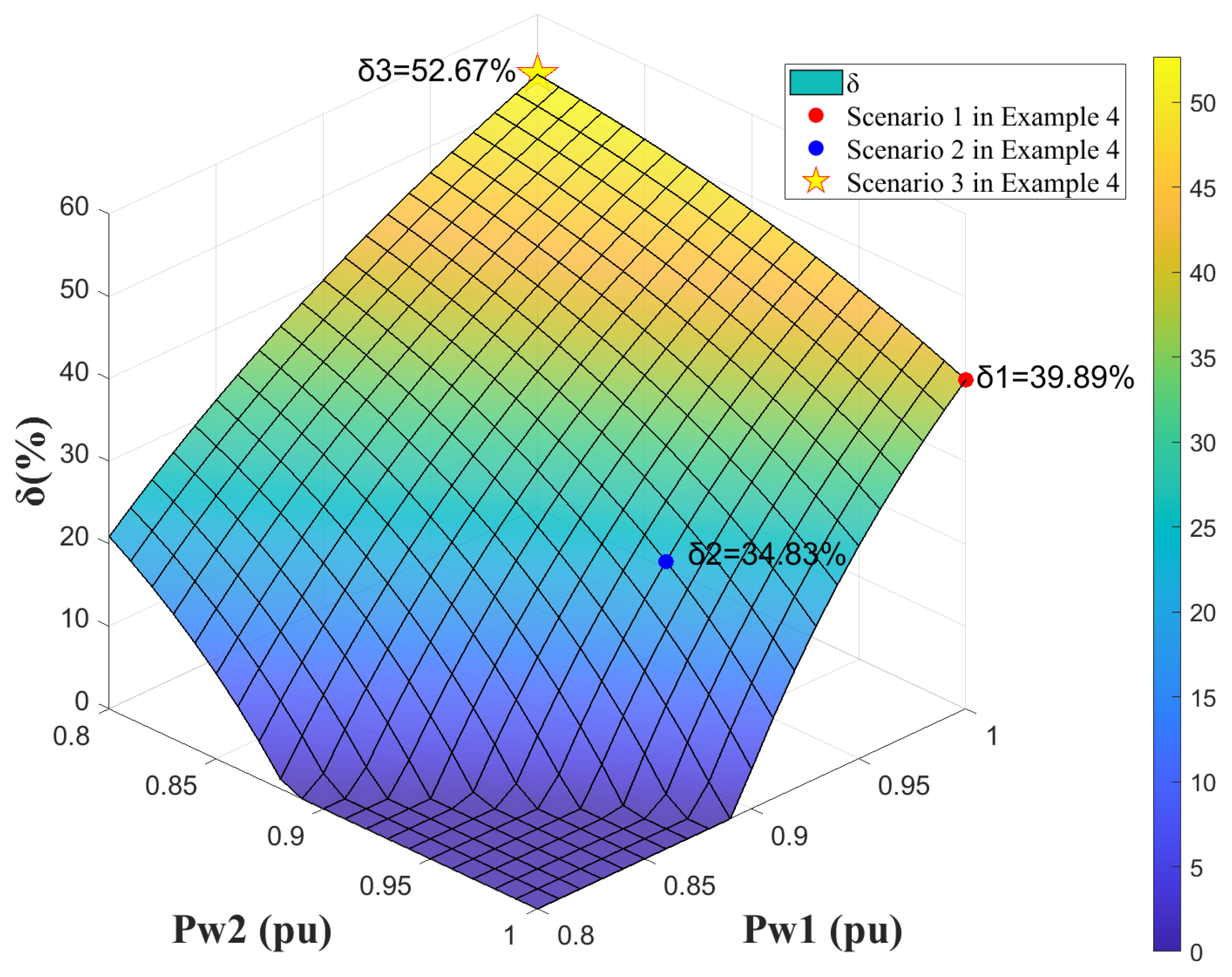
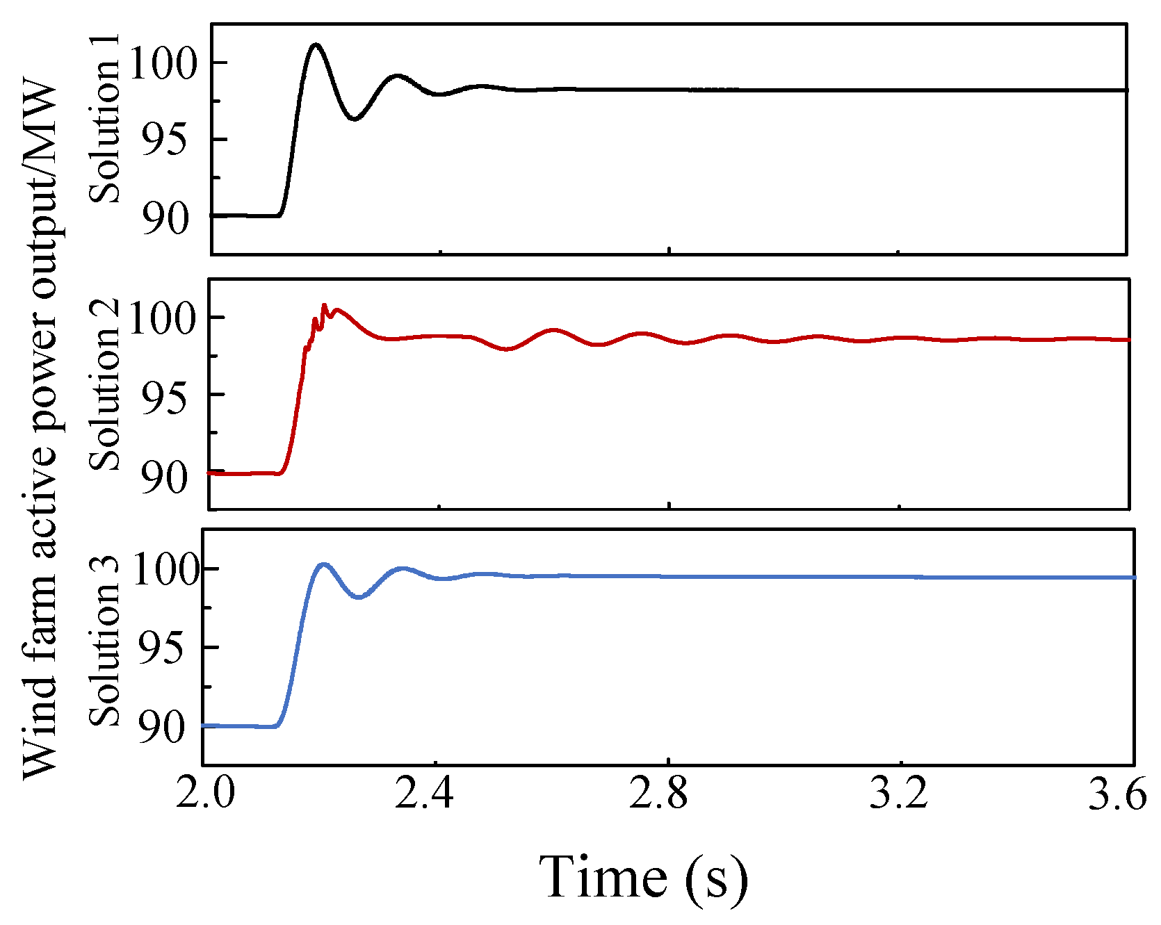
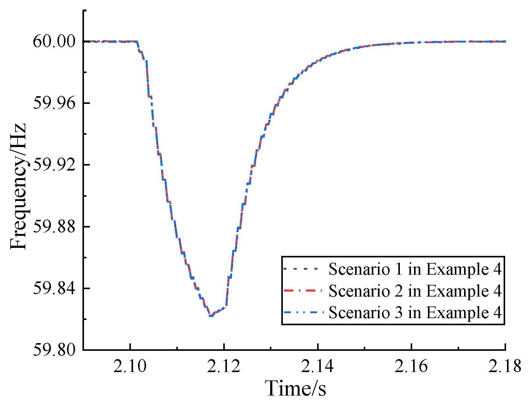
As shown in Figure 25, Figure 26 and Figure 27, under a 2.1 s frequency-modulated power disturbance, Scheme 3 exhibits the optimal transient response performance. It demonstrates the smallest overshoot in the wind farm’s active power output, the lowest oscillation amplitude, and the shortest recovery time, significantly outperforming Scheme 1 and Scheme 2. As shown in Figure 27, under Scheme 3, the system stability margin increases by 52.67%, which is 12.78% and 17.84% higher than Scheme 1 and Scheme 2, respectively, significantly enhancing the stability margin of the grid-connected system. Simultaneously, the frequency responses of all three schemes remained consistent. Although the wind farm scale increased, the total active power output remained unaffected across different schemes, with variations only occurring in the active power allocation between turbine clusters. Simulation results demonstrate that under various grid-connection scenarios, the proposed allocation schemes effectively optimize system response characteristics and enhance stability margins, exhibiting both good applicability and effectiveness. For the large-scale wind farm system in Example 4, comprising 50 wind turbines,

Table 8. Quantitative Comparison Table of Different Schemes in Example 4.

Performance Indicator	Equal Distribution	Capacity-Based Allocation	Proposed Strategy
Damping ratio stability margin	39.89%	34.83%	52.67%
Transient recovery time (s)	2.74	3.95	2.51
Active power overshoot (%)	2.6	3.1	2.0

further integrates and quantifies the performance differences among the three schemes under frequency regulation requirements:

6. Conclusions

This paper addresses the issue of enhancing stability during wind farms’ participation in system frequency regulation by proposing an optimized power allocation strategy for multi-turbine frequency regulation. Key conclusions are as follows:

(1)

A small-signal impedance model for wind farm grid-connected systems was established, accounting for unit output and terminal impedance variations. This model reveals the mechanism and matching relationship between active power output and terminal impedance in influencing stability margin.

(2)

A multi-turbine frequency regulation power allocation model is constructed to maximize the system damping ratio stability margin while accounting for power balance constraints and turbine active power output limitations, achieving coordinated optimization that balances frequency regulation power requirements with enhanced grid stability for wind farms;

(3)

Finally, considering practical and critical scenarios in power system operation, such as grid parameter changes caused by grid restructuring, load fluctuations, or line switching, we will explore the adaptability of the proposed strategy under dynamic grid conditions in a future study. Subsequent research will focus on extending this strategy to accommodate dynamic grid environments by integrating real-time grid impedance monitoring capabilities. This enhancement will improve the adaptability of the optimization strategy, enabling dynamic adjustments to power allocation schemes. The goal is to ensure the strategy maintains optimal stability margins while rapidly responding to grid parameter changes. The performance of the improved strategy will be validated through simulations and experimental testing under dynamic grid scenarios.

References

1. Staffell, I.; Pfenninger, S. The increasing impact of weather on electricity supply and demand. Energy 2018, 145, 65–78. [Google Scholar] [CrossRef]
2. National Energy Administration. 2024 Renewable Energy Grid Connection and Operation Status. Available online: http://www.chinapower.com.cn/sj/ndsj/20250206/276129.html (accessed on 1 July 2025).
3. Denholm, P.; Mai, T.; Kenyon, R.W.; Kroposki, B.; O’Malley, M. Inertia and the Power Grid: A Guide Without the Spin; National Renewable Energy Lab. (NREL): Golden, CO, USA, 2020. [Google Scholar]
4. Lasseter, R.H.; Chen, Z.; Pattabiraman, D. Grid-Forming Inverters: A Critical Asset for the Power Grid. IEEE J. Emerg. Sel. Top. Power Electron. 2020, 8, 925–935. [Google Scholar] [CrossRef]
5. Haque, M.E.; Paul, S.; Sheikh, M.R.I. Grid frequency analysis with the issue of high wind power penetration. In Proceedings of the 2013 International Conference on Electrical Information and Communication Technology (EICT), Khulna, Bangladesh, 13–15 February 2014; pp. 1–7. [Google Scholar]
6. Zhao, H.; Zhao, J.; Qiu, J.; Liang, G.; Dong, Z.Y. Cooperative Wind Farm Control with Deep Reinforcement Learning and Knowledge-Assisted Learning. IEEE Trans. Ind. Inform. 2020, 16, 6912–6921. [Google Scholar] [CrossRef]
7. Wang, D.; Liang, L.; Lei, S.; Hu, J.B.; Hou, Y.H. Analysis of modal resonance between PLL and DC-Link voltage control in weak-grid tied VSCs. IEEE Trans. Power Syst. 2019, 34, 1127–1138. [Google Scholar] [CrossRef]
8. Murcia Leon, J.P.; Koivisto, M.J.; Sørensen, P.; Magnant, P. Power fluctuations in high-installation- density offshore wind fleets. Wind Energy Sci. 2021, 6, 461–476. [Google Scholar] [CrossRef]
9. Yadav, V.V.; Saravanan, B. Technical advances and stability analysis in wind-penetrated power generation systems—A review. Front. Energy Res. 2022, 10, 986. [Google Scholar] [CrossRef]
10. Du, W.J.; Wang, Y.J.; Wang, H.F.; Ren, B.X.; Xiao, X.Y. Small-Disturbance Stability Limit of a Grid-Connected Wind Farm with PMSGs in the Timescale of DC Voltage Dynamics. IEEE Trans. Power Syst. A Publ. Power Eng. Soc. 2021, 36, 1623–1633. [Google Scholar] [CrossRef]
11. Du, W.; Ren, B.; Wang, H.; Wang, Y. Comparison of methods to examine Sub-synchronous oscillations caused by grid-connected wind turbine generators. IEEE Trans. Power Syst. 2019, 34, 4931–4943. [Google Scholar] [CrossRef]
12. Wu, L.; Xu, M.; Lin, J.; Xu, H.; Zheng, L. Active Power Dispatch of Renewable Energy Power Systems Considering Multiple Renewable Energy Station Short-Circuit Ratio Constraints. Electronics 2024, 13, 3811. [Google Scholar] [CrossRef]
13. Chai, Z.S.; Li, H.; Xie, X.R.; Abdeen, M.; Yang, T.; Wang, K. Output impedance modeling and grid-connected stability study of virtual synchronous control-based doubly-fed induction generator wind turbines in weak grids. Int. J. Electr. Power Energy Syst. 2021, 126, 106601. [Google Scholar] [CrossRef]
14. Cespedes, M.; Sun, J. Impedance modelling and analysis of grid-connected voltage-source converters. IEEE Trans. Power Electron. 2014, 29, 1254–1261. [Google Scholar] [CrossRef]
15. Du, W.; Dong, W.; Wang, H. A Method of Reduced-Order Modal Computation for Planning Grid Connection of a Large-Scale Wind Farm. IEEE Trans. Sustain. Energy 2020, 11, 1185–1198. [Google Scholar] [CrossRef]
16. Shao, B.; Zhao, S.; Gao, B.; Yang, Y.; Blaabjerg, F. Adequacy of the Single-Generator Equivalent Model for Stability Analysis in Wind Farms With VSC-HVDC Systems. IEEE Trans. Energy Convers. 2021, 36, 907–918. [Google Scholar] [CrossRef]
17. Tao, S.; Zhao, L.; Liu, Y.; Liao, K. Impedance Network Model of D-PMSG Based Wind Power Generation System Considering Wind Speed Variation for Sub-synchronous Oscillation Analysis. IEEE Access 2020, 8, 114784–114794. [Google Scholar] [CrossRef]
18. Wu, D.; Seo, G.-S.; Xu, L.; Su, C.; Kocewiak, L.; Sun, Y.; Qin, Z. Grid Integration of Offshore Wind Power: Standards, Control, Power Quality and Transmission. IEEE Open J. Power Electron. 2024, 5, 583–604. [Google Scholar] [CrossRef]
19. Du, W.; Dong, W.; Wang, H.F. Small-Signal Stability Limit of a Grid-Connected PMSG Wind Farm Dominated by the Dynamics of PLLs. IEEE Trans. Power Syst. 2020, 35, 2093–2107. [Google Scholar] [CrossRef]
20. Bao, W.; Wu, Q.; Ding, L.; Huang, S.; Terzija, V. A Hierarchical Inertial Control Scheme for Multiple Wind Farms With BESSs Based on ADMM. IEEE Trans. Sustain. Energy 2021, 12, 751–760. [Google Scholar] [CrossRef]
21. Wang, P.; Wu, Q.; Huang, S.; Li, C.; Zhou, B. ADMM-based Distributed Active and Reactive Power Control for Regional AC Power Grid with Wind Farms. J. Mod. Power Syst. Clean Energy 2022, 10, 588–596. [Google Scholar] [CrossRef]
22. Ding, R.; Yang, C.; Mei, R.; Yang, H.; Ji, J.; Shi, Q. Research on simplified modeling of large-scale wind farms based on equivalent transfer function and aggregate equivalent. Front. Energy Res. 2023, 10, 1098025. [Google Scholar] [CrossRef]
23. Li, C. Frequency modulation technology for power systems incorporating wind power, energy storage, and flexible frequency modulation. Sustain. Energy Res. 2025, 12, 10. [Google Scholar] [CrossRef]
24. Jiang, C.; Cai, G.; Yang, D.; Liu, X.; Hao, S.; Li, B. Multi-objective configuration and evaluation of dynamic virtual inertia from DFIG based wind farm for frequency regulation. Int. J. Electr. Power Energy Syst. 2024, 158, 109956. [Google Scholar] [CrossRef]
25. Astapov, V.Y. Applicability of multi-agent control for virtual inertia modes in a wind power plant. iPolytech J. 2024, 27, 694–726. [Google Scholar] [CrossRef]
26. Feleke, S.; Satish, R.; Pydi, B.; Anteneh, D.; Abdelaziz, A.Y.; El-Shahat, A. Damping of Frequency and Power System Oscillations with DFIG Wind Turbine and DE Optimization. Sustainability 2023, 15, 4751. [Google Scholar] [CrossRef]
27. Li, Y.; Zhu, G.; Lu, J.; Geng, H. Voltage Support Capacity Improvement for Wind Farms with Reactive Power Substitution Control. CSEE J. Power Energy Syst. 2025, 11, 999–1017. [Google Scholar]
28. Yao, Q.; Hu, Y.; Deng, H. Two-degree-of-freedom active power control of megawatt wind turbine considering fatigue load optimization. Renew. Energy 2020, 162, 2096–2112. [Google Scholar] [CrossRef]
29. Yao, Q.; Liu, J.; Hu, Y. Optimized active power dispatching strategy considering fatigue load of wind turbines during de- loading operation. IEEE Access 2019, 7, 17439–17449. [Google Scholar] [CrossRef]
30. GB/T 40581-2021; Calculation Specification for Power System Security and Stability. State Administration for Market Regulation, Standardization Administration of China: Beijing, China, 2021.
31. Li, W.; Li, Y.; Li, J.; Zhang, Y.; Chang, X.; Sun, Z. Variable droop gain frequency supporting control with maximum rotor kinetic energy utilization for wind-storage system. Int. J. Electr. Power Energy Syst. 2024, 163, 110289. [Google Scholar] [CrossRef]
32. Kim, T.; Kim, C.; Song, J.; You, D. Optimal control of a wind farm in time-varying wind using deep reinforcement learning. Energy 2024, 303, 131950. [Google Scholar] [CrossRef]
Figure 1. Grid-connected Topology and Control Diagram of PMSG.
Sustainability 18 01406 g001
Figure 2. Small-signal Control Path of PMSG.
Sustainability 18 01406 g002
Figure 3. Equivalent Impedance Model for Grid-Connected Single Wind Turbine.
Sustainability 18 01406 g003
Figure 4. Equivalent Impedance Model for Grid-Connected Wind Farms.
Sustainability 18 01406 g004
Figure 5. Gridconnected System Amplitudephase Characteristic Curve When Active Output Changes.
Sustainability 18 01406 g005
Figure 6. Nyquist Curve of The Gridconnected System When Active Output Changes.
Sustainability 18 01406 g006
Figure 7. Amplitude-phase Characteristic Curve of Grid-connected System When XL Is Changed.
Sustainability 18 01406 g007
Figure 8. Nyquist Curve of The Grid-connected System When XL Is Changed.
Sustainability 18 01406 g008
Figure 9. Amplitude-Phase Characteristics of Wind Turbine under Varying Active Power Outputs at XL = 0.02.
Sustainability 18 01406 g009
Figure 10. Amplitude-Phase Characteristics of Wind Turbine under Varying Active Power Outputs at XL = 0.001.
Sustainability 18 01406 g010
Figure 11. Nyquist Plots of Grid-Connected Systems Configured with Varying Active Power Outputs under Two Typical Operating Scenarios.
Sustainability 18 01406 g011
Figure 12. Scenario 1 Amplitude-phase Characteristic Curve.
Sustainability 18 01406 g012
Figure 13. Scenario 2 Amplitude-phase Characteristic Curve.
Sustainability 18 01406 g013
Figure 14. Scenario 3 Amplitude-phase Characteristic Curve.
Sustainability 18 01406 g014
Figure 15. Comparison of Nyquist-Curves Under Different Scenarios.
Sustainability 18 01406 g015
Figure 16. Schematic Diagram of Frequency Regulation Power Allocation in Wind Farms.
Sustainability 18 01406 g016
Figure 17. Sweep Result Graph.
Sustainability 18 01406 g017
Figure 18. Figure 1 of Example 2 Results.
Sustainability 18 01406 g018
Figure 19. Figure 2 of Example 2 Results.
Sustainability 18 01406 g019
Figure 20. Example 3 Simulation System Topology Diagram.
Sustainability 18 01406 g020
Figure 21. Example 3 Results Diagrams.
Sustainability 18 01406 g021aSustainability 18 01406 g021b
Figure 22. Frequency Response Plot.
Sustainability 18 01406 g022
Figure 23. Stability Margin Versus Output Distribution.
Sustainability 18 01406 g023
Figure 24. Example 4 Simulation System Topology Diagram.
Sustainability 18 01406 g024
Figure 25. Wind Farm Output Active Power Diagram.
Sustainability 18 01406 g025
Figure 26. Frequency Response Plot.
Sustainability 18 01406 g026
Figure 27. Stability Margin Versus Output Distribution.
Sustainability 18 01406 g027