Agro-Environmental Vulnerability and Ecosystem Sustainability in Peruvian Family Farming: Integrating Survey Data, Spatial Modeling and Remote Sensing

Abstract

Subsistence family farming in Peru is increasingly constrained by ecosystem degradation, climate variability, and limited access to productive services, particularly where environmental exposure is high. This study develops an Agro-productive and Territorial Vulnerability Index (IVAPT) to evaluate environmental, ecosystem, and socioeconomic vulnerability of subsistence agriculture at the district level nationwide. The index integrates district-level agricultural survey data (ENA-2024) with multi-temporal MODIS NDVI series (2000–2024) and comprehensive climatic, topographic, land-cover, and accessibility indicators, processed through multivariate statistics. Three objective weighting schemes (ENTROPY, CRITIC, PCA) construct thematic sub-indices of Environmental Exposure (EnvExp), Ecosystem Condition (EcoCond), and Socioeconomic Capacity (SocioCap). Results show more than half of Peru’s 1552 districts fall within moderate to very high vulnerability, with highest concentration in the Amazon region (Loreto, Ucayali, Madre de Dios), Andean-Amazonian transitions, and highland districts (Huancavelica, Apurímac, Ayacucho, Puno) where biophysical constraints, ecosystem pressure, and socioeconomic isolation converge. Dimensional spatial complementarity EnvExp peaking on coast, EcoCond in Amazon, SocioCap in Andes demonstrates effective vulnerability reduction requires dimension-specific interventions. Despite divergent weighting schemes, spatial patterns remained consistent, validating identified hotspots. IVAPT provides a reproducible framework supporting evidence-based territorial planning and targeted investments in water infrastructure, ecosystem restoration, and climate adaptation.

1. Introduction

Agriculture is a fundamental component of economic development and is closely linked to several Sustainable Development Goals (SDGs), including Goals 2, 6, 8, 10, 12, 13, and 15, which emphasize the need to evaluate its sustainability [1]. It also remains a key pillar of the global economy and plays an important role in food security and in supporting rural livelihoods [2]. For most rural households, agricultural activity represents not only a source of income but also a central element of subsistence, social cohesion, and cultural identity [3]. However, climate change is one of the main challenges facing the agricultural sector because it alters temperature and weather conditions and increases the vulnerability of small farmers and communities that depend on agricultural production [4]. This situation is further affected by the projected growth of the global population, which is expected to reach nearly 10 billion people by 2050 and will require a 50 percent increase in food production compared to 2013 levels, reinforcing the need to strengthen the resilience and sustainability of agricultural systems [2]. In this context, there is increasing agreement on the urgent need to transform agricultural systems toward more sustainable and resilient production models that can reduce their vulnerability to climate variability and respond effectively to the environmental, social, and production challenges of the future [5].

Agro-environmental vulnerability represents the degree to which productive systems and the ecosystems that support them are affected by climatic variations, considering their exposure, sensitivity, and adaptive capacity [6]. This approach recognizes the close interdependence between the social, economic, and ecological components of a territory, highlighting that environmental degradation and the loss of soil resilience increase the susceptibility of agricultural systems [7]. In recent years, the intensification of natural disasters has significantly affected agriculture, a sector that is particularly vulnerable to environmental variability [8]. In this context, developing regions could experience reductions of between 9 and 21 percent in agricultural productivity [6], while low- and lower-middle-income countries are already facing losses of around 15 percent of their total production [8]. These trends emphasize the need to strengthen adaptation strategies based on the sustainability of agroecosystems.

Agriculture plays a fundamental role in rural economies, as it forms the basis of food security, employment, and economic development in most developing countries. Its high dependence on weather conditions makes it one of the most vulnerable sectors to climate variability and extreme events [9]. Small-scale farms, which represent the majority of holdings worldwide and operate a limited portion of cultivated land, are essential for the sustainability of food systems, particularly in rural areas where they contribute significantly to food security and community livelihoods [10]. However, climatic phenomena such as droughts, heat waves, and floods are already affecting food production, and it is estimated that climate change could reduce the yields of staple crops by up to 30 percent due to lower productivity and crop losses [11]. At the global level, both developing and emerging economies remain highly dependent on agriculture, which continues to be the main source of employment and a key driver of economic growth [12,13]. Furthermore, the use and scale of agricultural land reflect the ongoing transformation of rural territories, influencing production efficiency, environmental resilience, and livelihoods, and highlighting the need for balanced soil management aimed at sustainability [14].

In this context, family farming plays a strategic role within agri-food systems, as it directly contributes to food security and poverty reduction. Its multidimensional approach helps strengthen the resilience of production systems and improve rural livelihoods, which led the United Nations to declare the Decade of Family Farming (2019–2028) to highlight its key role in the sustainable transformation of the agricultural sector [15,16]. In Peru, agriculture also plays a strategic role as one of the main drivers of rural development. It is characterized by a marked productive heterogeneity, combining modernized systems with small-scale units that are highly dependent on natural resources [17,18]. Family farming, which represents more than 95 percent of the country’s agricultural units, integrates production and family life into a single system with strong social, economic, cultural, and environmental links. It concentrates on the majority of agricultural employment and forms the core of the national food system. It is also supported by peasant and native communities that manage their lands and adapt to changing environmental conditions, reaffirming their role as a pillar of economic, social, and environmental sustainability in rural areas [19,20,21].

Subsistence family farming in Peru forms the foundation of livelihood for millions of people, especially in the Andean highlands and Amazonian regions. According to the National Agricultural Survey [22], more than 50 percent of Agricultural Production Units (UPAs) operate on less than 3 hectares and generate incomes below the poverty threshold. These units are characterized by limited access to services, low levels of mechanization, restricted production diversification, and a high dependence on climatic factors. Despite their importance for national food security, they show high vulnerability to climatic variations and environmental pressures, which is expressed in three main dimensions: environmental, due to soil degradation, loss of agrobiodiversity, and water scarcity; economic, due to low profitability and limited access to resources, infrastructure, and markets; and social, due to land fragmentation, lack of technical assistance, and low adaptive capacity among small producers [23,24]. On the other hand, its complex geography, exposure to hazards such as droughts, frosts, floods, and landslides, and the strong dependence on subsistence family farming factors that limit its adaptive capacity and increase both environmental and socioeconomic risks [25].

Although there have been institutional advances such as the National Map of Agricultural Surface [26] and georeferenced databases from National Institute of Statistics and Informatics (INEI) and National Geographic Institute (IGN), information on these vulnerabilities remains fragmented, limiting the development of effective public policies. Despite the increasing availability of agricultural surveys, satellite imagery, and geospatial databases, there remains a clear lack of integrated spatial–statistical frameworks at the district level that systematically combine socioeconomic, environmental, and ecosystem information into a single, operational vulnerability metric. This fragmentation restricts comparability across territories and constrains the effective targeting of territorial planning, climate adaptation, and ecosystem restoration policies. Among these efforts, several studies [27,28] highlight the usefulness of multivariate approaches and synthetic indices for mapping critical territories. Among these, the Normalized Difference Vegetation Index (NDVI) has proven to be an effective tool for evaluating vegetation productivity and detecting long-term environmental degradation [29,30]. Nevertheless, Peru still lacks an integrated Agro-Productive and Territorial Vulnerability Index (IVAPT) that combines census-based, satellite-derived, and spatial information within a unified analytical framework.

In this context, the present research aims to characterize and map the structural, environmental, and territorial vulnerability of subsistence family farming in Peru by integrating productive, socioeconomic, biophysical, and geospatial data through spatial analysis techniques and remote sensing tools. Specifically, the study seeks to classify subsistence UPAs based on variables such as agricultural income, cultivated area, degree of production diversification, and access to basic services, using data from the National Agricultural Surveys (ENA) conducted by the National Institute of Agricultural Innovation (INIA). It also analyzes the temporal evolution of the NDVI (2000–2024) as a proxy indicator of vegetation productivity to assess degradation or improvement trends in agricultural areas. Furthermore, it designs and calculates a composite multivariate vulnerability index that integrates structural, environmental, and territorial dimensions at the district level, incorporating complementary geographic variables such as road network density, distance to water bodies, lake density, topographic diversity, and agricultural surface per district. The identification of critical areas and differentiated vulnerability patterns is based on the spatial distribution and classification of the composite index and its thematic sub-indices. Although the analysis is focused on Peru, the proposed methodological framework is inherently scalable and transferable to other countries and regions with similar data structures. By relying on widely available agricultural surveys, open-access remote sensing products, and standard geospatial indicators, the IVAPT can be adapted to other Andean, tropical, or developing regions by adjusting indicator selection and administrative units while preserving its core analytical structure.

This research represents a opportunity to advance territorial understanding of subsistence family farming in Peru by leveraging the analytical potential of the ENA and complementary geospatial datasets. By integration of productive, socioeconomic, and spatial information within a coherent, district-level framework, the study contributes to overcoming the traditionally fragmented approaches used to assess agro-environmental vulnerability and provides a robust basis for evidence-based territorial planning and sustainable rural development.

2. Materials and Methods

2.1. Study Area

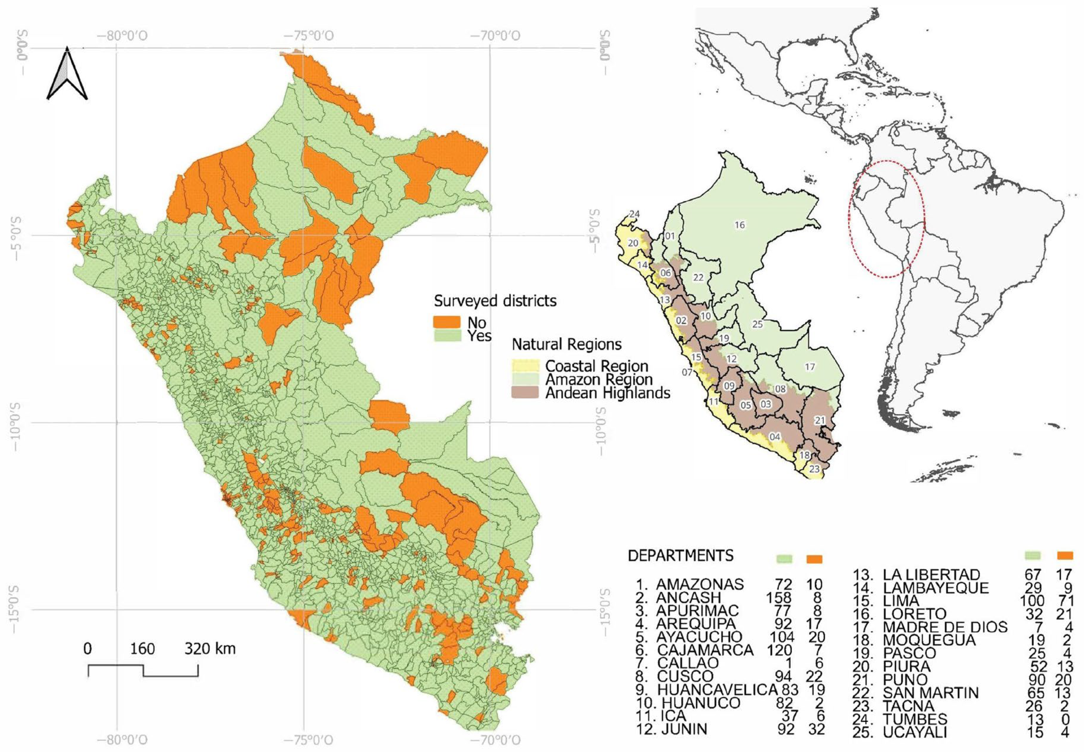
The present study was conducted on a representative sample of the national territory, considering that Peru is divided into 25 departments and 1891 districts distributed across three main geographical regions: the coast, the Andean highlands, and the Amazon rainforest (Figure 1). The coastal region is characterized by an arid and temperate climate, with a high concentration of intensive agricultural production supported by technified irrigation systems. The Andean highlands exhibit a temperate-to-cold and seasonal climate, where subsistence family farming predominates on slopes and inter-Andean valleys. Meanwhile, the Amazon region features a humid tropical climate, in which agricultural activity coexists with agroforestry systems and high biodiversity conditions. In this context, the analysis was based on information collected from 1552 districts, corresponding to those with valid and comparable data from the National Agricultural Survey (ENA-2024), while the remaining districts were excluded due to the absence of relevant agricultural activity, predominantly urban characteristics, or lack of consistent records [23,31].

At the national level, agricultural activity in Peru is distributed heterogeneously, reflecting the country’s ecological, cultural, and productive diversity. However, there are regions where family farming plays a particularly significant role and constitutes the foundation of rural livelihoods. Departments such as Cajamarca, Junín, Puno, Cusco, Ayacucho, Huánuco, La Libertad, Piura, and San Martín stand out for their high concentration of agricultural units, extensive cultivated areas, and strong contribution to national food security. These regions combine favorable biophysical conditions, well-established agricultural traditions, and a high dependence on local natural resources, making them representative of the country’s agrarian dynamics. In most of these territories, family farming maintains a leading role in food production, rural employment generation, and the conservation of agroecological landscapes, positioning itself as an essential component for understanding the structure and vulnerability of the Peruvian agricultural system [19,32,33].

2.2. National Agricultural Survey

The main source of information was the 2024 ENA [34], conducted jointly by the Ministry of Agricultural Development and Irrigation (MIDAGRI) and INEI. The ENA is a nationwide sample survey designed to ensure statistical representativeness at the national and departmental levels, and in some cases at the provincial level, but it is not an agricultural census and does not ensure comprehensive coverage of all districts in the country.

In this research, the ENA-2024 data were used as the input for analyzing and characterizing the vulnerability of subsistence family farming in Peru at the district level, considering only those districts that had valid, consistent, and comparable information for the socioeconomic modules included in the analysis. In this context, the ENA exclude districts that: (i) are located in desert areas without significant agricultural activity; (ii) are predominantly urban (100% urban area); (iii) correspond to Amazonian districts without agricultural records; (iv) have a small agricultural area that does not meet the minimum statistical thresholds required for a robust estimation of indicators; or (v) have an extremely low rural population.

2.3. Remote and Special Information

To complement the socioeconomic information from ENA-2024, a set of environmental and territorial variables was derived from remote sensing and geospatial datasets processed through digital platforms. The analysis used Moderate Resolution Imaging Spectroradiometer (MODIS, ID: MOD13Q1) images accessed through [35] accessed via Google Earth Engine (GEE) [36] to generate long-term NDVI time series (2000–2024) with a resolution of 250 m and 16-day temporal resolution. Topographic parameters such as mean altitude and slope were obtained from the Shuttle Radar Topography Mission (SRTM, NASA/USGS) at 30 m spatial resolution. Additional spatial data were integrated from the National Water Authority (ANA) and the IGN to calculate the distance to surface water bodies and road density, while land cover diversity was estimated using the MapBiomas Peru dataset. Territorial accessibility was derived from the Global Accessibility Map [37], and rural population density was obtained from the 2017 National Census the INEI.

To ensure consistency with the socioeconomic information from ENA-2024, all spatial indicators were harmonized to the 2024 reference year by using the most recent versions available of each dataset or, in the case of time-series variables, by summarizing long-term trends representative of current conditions. All spatial layers were subsequently aggregated and standardized at the district level, enabling direct comparability with the ENA-based indicators and ensuring a coherent integration of socioeconomic, environmental, and territorial information within the vulnerability assessment framework [38,39,40]. The detailed method of calculating all variables mentioned in Section 2.2 and Section 2.3 is provided in Appendix A,

Table A1. Description, calculation method, and data source of variables used to build the Vulnerability Index.

Variable	Group	Description/Calculation Method	Source
PrecMn, PrecMe, PrecMx, PrecSD	Environmental Exposure	Mean, median, maximum and standard deviation of annual precipitation (2000–2024) aggregated from monthly grids.	CHIRPS v2.0/WorldClim v2
ElevMn–ElevSD	Environmental Exposure	Elevation statistics (mean, sd, min, max m a.s.l.) derived from 30 m DEM.	SRTM DEM 30 m
SlpMn–SlpSD	Environmental Exposure	Slope metrics (mean, sd, min, max in degrees) derived from DEM terrain functions.	SRTM DEM 30 m
DstCPm, DstCSD, DstRMe, DstRSD, DstLMe, DstLSD	Environmental Exposure	Mean and variability of Euclidean distance (km) to population centers, rivers and lakes.	MTC—2024/GEE distance analysis
HPIMe, HPISD	Environmental Exposure	Hydrological Proximity Index − mean and sd of distance from each pixel to nearest water body; lower values = greater hydrological influence.	GEE hydrological distance layer (ANA 2020 hydrography + MapBiomas water class)
PDSIMe–PDSIMn2	Environmental Exposure	Precipitation Deficit Severity Index (PDSI) statistics (mean, sd, min, max) for 2000–2024.	CHIRPS/TerraClimate
DrtFrq, DrtSD	Environmental Exposure	Drought frequency and variability based on negative NDVI anomalies (2000–2024).	MODIS MOD13Q1
AgrAr	Ecosystem Condition	Percentage of district area under agriculture, based on MIDAGRI 2025 national land-use inventory.	MIDAGRI (2025 Inventory [26])
ImpSg, ImpSl, Stabl, DegSl, DegSg, PImp, PSta, PDeg	Ecosystem Condition	Percentage of improved, stable and degraded pasture classes derived from NDVI trend categories.	MODIS NDVI 2000–2024
ShNDVI	Ecosystem Condition	Diversity of vegetation response, computed as Shannon entropy of NDVI trend classes within each district.	MODIS MOD13Q1 (2000–2024)
ShMBio, EvMBio	Ecosystem Condition	Land-cover heterogeneity indices capturing the diversity and evenness of MapBiomas land-cover types (based on biomass and evapotranspiration proxies).	MapBiomas Peru v9/MOD16A2
TMean	Ecosystem Condition	Travel time mean (min)—average time to reach the nearest urban center by road network; proxy for accessibility and service connectivity.	Accessibility to Cities (Global Friction Surface v2/Weiss et al., 2018 [37])
TMax	Ecosystem Condition	Maximum travel time to urban centers within the district (upper bound of accessibility).	Same as above
RdDep, RdNat, RdMin, RdTot	Ecosystem Condition	Total length of departmental, national, minor and total roads (km) aggregated by district and normalized by district area (km2) to obtain road density.	MTC Road Network/OpenStreetMap
NBI	Ecosystem Condition	Net Balance Index (NBI) = (% Improvement − % Degradation) from NDVI trend analysis (positive = greening dominates; negative = degradation).	MODIS NDVI 2000–2024/custom trend classification
IncUA	Socioeconomic Capacity	Per capita agricultural income (log-transformed and standardized).	ENA 2024 Module 6 [34]
DivAg, DivPe	Socioeconomic Capacity	Crop and livestock diversification indices (Herfindahl–Simpson index).	ENA 2024 Modules 3–5 [34]
SupUA	Socioeconomic Capacity	Access to agricultural support services (% UPA with support).	ENA 2024 Module 8 [34]
Train, TechAs	Socioeconomic Capacity	Access to training and technical assistance (% UPA).	ENA 2024 Module 8 [34]
TenArr–TenOth	Socioeconomic Capacity	Land tenure structure (% UPA by ownership type: rent, own, communal, possession, other).	ENA 2024 Module 2 [34]
BPAAg, BPAPe	Socioeconomic Capacity	Belonging to producer associations or cooperatives (% UPA).	ENA 2024 Module 9 [34]
Assoc	Socioeconomic Capacity	Membership in local organizations (% UPA).	ENA 2024 Module 9 [34]
CredRq, CredOk	Socioeconomic Capacity	Percentage of UPA that requested and obtained credit.	ENA 2024 Module 10 [34]
Equip, Machn, Irrig	Socioeconomic Capacity	Access to equipment, machinery and irrigation infrastructure (% UPA).	ENA 2024 Modules 7 and 8 [34]

.

2.4. Variables and Indicators by Analytical Dimension

Indicator selection followed a conceptual and empirical framework of agro-environmental vulnerability integrating environmental exposure, ecosystem condition, and socioeconomic adaptive capacity. Indicators were compiled from agricultural surveys, remote sensing products, climatic datasets, and national geospatial databases to capture vulnerability at the district scale. Selection criteria included theoretical relevance, empirical interpretability, national-scale data availability, and compatibility with multivariate analysis, consistent with previous multidimensional vulnerability assessments [5,41,42,43]. Prior to correlation analysis and aggregation, all indicators were harmonized to ensure consistent directionality with respect to vulnerability. Cost-type indicators are those for which higher values indicate higher vulnerability (e.g., climatic variability, drought frequency, topographic constraints, distance to water bodies), whereas benefit-type indicators are those for which higher values indicate lower vulnerability (e.g., income, infrastructure, irrigation, diversification, and technical assistance). Benefit-type indicators were reverse-scaled after min–max normalization, so that higher values uniformly represented higher vulnerability (

Table 1. Environmental exposure.

Subgroup	Variables	Meaning/Interpretation	Directionality (Vulnerability)
Climatic variability	PrecMn	Mean annual precipitation	Benefit (−)
	PrecMe	Median annual precipitation	Benefit (−)
	PrecMx	Maximum annual precipitation	Benefit (−)
	PrecSD	Interannual precipitation variability	Cost (+)
Topographic stress	ElevMn	Mean elevation	Cost (+)
	ElevMe	Median elevation	Cost (+)
	ElevMx	Maximum elevation	Cost (+)
	ElevSD	Elevation variability	Cost (+)
	SlpMn	Mean slope	Cost (+)
	SlpMe	Median slope	Cost (+)
	SlpMx	Maximum slope	Cost (+)
	SlpSD	Slope variability	Cost (+)
Hydro-climatic proximity	DstCPm	Mean distance to permanent water bodies	Cost (+)
	DstCSD	SD of distance to permanent water bodies	Cost (+)
	DstRMe	Mean distance to rivers	Cost (+)
	DstRSD	SD of distance to rivers	Cost (+)
	DstLMe	Mean distance to lakes	Cost (+)
	DstLSD	SD of distance to lakes	Cost (+)
	HPIMe	Mean Hydrological Proximity Index	Benefit (−)
	HPISD	Variability of Hydrological Proximity Index	Cost (+)
Drought stress (PDSI)	PDSIMe	Mean Palmer Drought Severity Index	Benefit (−)
	PDSISD	Variability of PDSI	Cost (+)
	PDSIMn	Minimum PDSI	Cost (+)
	PDSIMe2	Mean PDSI (2000–2010)	Benefit (−)
	PDSIMx	Maximum PDSI	Benefit (−)
	PDSISD2	SD of PDSI (2000–2010)	Cost (+)
	PDSIMn2	Minimum PDSI (2000–2010)	Cost (+)
	DrtFrq	Frequency of drought events	Cost (+)
	DrtSD	Variability of drought frequency	Cost (+)

Note: For PDSI-based indicators, higher values represent wetter conditions and lower drought stress; therefore, mean and maximum PDSI metrics were treated as benefit-type indicators, while minimum values and variability metrics were treated as cost-type indicators.

,

Table 2. Ecosystem condition and land dynamics.

Subgroup	Variables	Meaning/Interpretation	Directionality (Vulnerability)
Land-use intensity	AgrAr	Total agricultural area per district	Cost (+)
NDVI trend classes	ImpSg	Significant vegetation improvement	Benefit (−)
	ImpSl	Slight vegetation improvement	Benefit (−)
	Stabl	Stable vegetation trend	Benefit (−)
	DegSl	Slight vegetation degradation	Cost (+)
	DegSg	Significant vegetation degradation	Cost (+)
NDVI balance indices	PImp	Proportion of improvement	Benefit (−)
	PSta	Proportion of stability	Benefit (−)
	PDeg	Proportion of degradation	Cost (+)
	NBI	NDVI Balance Index	Benefit (−)
Diversity of vegetation response	ShNDVI	Shannon index of NDVI change	Benefit (−)
Land-cover heterogeneity	ShMBio	Shannon diversity of MapBiomas land-cover classes	Benefit (−)
	EvMBio	Evenness of MapBiomas land-cover classes	Benefit (−)
Accessibility/connectivity	TMean	Mean travel time to urban centers	Cost (+)
	TMax	Maximum travel time	Cost (+)
	RdDep	Length of departmental roads	Benefit (−)
	RdNat	Length of national roads	Benefit (−)
	RdMin	Length of minor/local roads	Benefit (−)
	RdTot	Total road length	Benefit (−)

and

Table 3. Socioeconomic Capacity and adaptive capacity.

Subgroup	Variables	Meaning/Interpretation	Directionality (Vulnerability)
Income & productive structure	IncUA	Average income per UPA	Benefit (−)
	DivAg	Agricultural diversification index	Benefit (−)
	DivPe	Livestock diversification index	Benefit (−)
	SupUA	Average productive area per UPA	Benefit (−)
Tenure & land management	TenArr	Proportion of rented land	Cost (+)
	TenOwn	Proportion of owned land	Benefit (−)
	TenCom	Proportion of communal land	Cost (+)
	TenPos	Proportion of possessed (informal) land	Cost (+)
	TenOth	Other tenure types	Cost (+)
Good agricultural & livestock practices	BPAAg	Adoption of good agricultural practices	Benefit (−)
	BPAPe	Adoption of good livestock practices	Benefit (−)
Access & modernization	Equip	Availability of agricultural equipment	Benefit (−)
	Machn	Level of mechanization	Benefit (−)
	Irrig	Access to irrigation	Benefit (−)
	Assoc	Participation in producer associations	Benefit (−)
	CredRq	Proportion of producers requesting credit	Cost (+)
	CredOk	Proportion of approved credit requests	Benefit (−)
Institutional & technical support	Train	Participation in agricultural training	Benefit (−)
	TechAs	Access to technical assistance	Benefit (−)

).

Table 1 summarizes the Environmental Exposure (EnvExp) dimension, including climatic variability, topographic stress, hydro-climatic proximity, and drought stress; in the latter, minimum, variability, and frequency-based PDSI metrics represent increased exposure, while higher mean and maximum PDSI values indicate wetter conditions and reduced exposure.

Table 2 presents the variables defining the Ecosystem Condition and Land Dynamics dimension, which characterizes the ecological status, vegetation stability, and landscape configuration across districts. Land-use intensity is represented by the total agricultural area (AgrAr), treated as a cost-type indicator reflecting pressure from land conversion and increased exposure to land-use stress. NDVI trend classes and balance indices capture the relative dominance of vegetation improvement, stability, or degradation based on long-term NDVI trajectories; higher proportions of improvement and stability are considered benefit-type indicators, whereas higher proportions of degradation indicate declining ecosystem condition and increased vulnerability (Appendix A,

Table A2. NDVI-based ecosystem changes metrics.

Metric	Computed From	Purpose/Interpretation
% Significant Improvement	(class 1 pixels/total) × 100	Spatial extent of robust greening
% Slight Improvement	class 2 pixels	Area with weak greening
% Stable	classes 3 + 6 pixels	Stable vegetation
% Slight Degradation	class 4 pixels	Early degradation signals
% Significant Degradation	class 5 pixels	Strong degradation “hot spots”
% Total Change	(1 + 2 + 4 + 5)/total	Share of area under change
NDVI Balance Index (NBI)	(% Improvement − % Degradation)	Positive = greening dominates; negative = degradation dominates
Shannon Entropy	Distribution across classes	Heterogeneity of responses inside the district

). The diversity of vegetation response (ShNDVI), measured using the Shannon index of NDVI change, reflects the heterogeneity of vegetation dynamics and is treated as a benefit-type indicator, as greater functional diversity is associated with enhanced ecosystem resilience. Land-cover heterogeneity (ShMBio and EvMBio), derived from MapBiomas land-cover classes, represents landscape diversity and evenness and is likewise treated as benefit-type indicators reflecting ecological complexity. Finally, accessibility and connectivity are described using travel time and road density metrics, where longer travel times constitute cost-type indicators and greater road availability represents benefit-type indicators associated with improved connectivity and reduced territorial isolation. Together, these indicators describe ecosystem condition and land dynamics that influence environmental resilience and land-use sustainability.

Table 3 presents the variables defining the Socioeconomic and Adaptive Capacity (Socio-Cap) dimension, which captures how productive structure, land tenure, modernization, and institutional support shape the vulnerability and resilience of agricultural systems. The income and productive structure subgroup includes indicators of average income, agricultural and livestock diversification, and productive area, all treated as benefit-type indicators reflecting the economic base and buffering capacity of farming units. Land tenure and management describe the distribution of tenure regimes, where higher shares of owned land are treated as benefit-type indicators associated with investment stability, whereas rented, informal, communal, or other tenure types are treated as cost-type indicators reflecting tenure insecurity and constraints on long-term land management. The adoption of good agricultural and livestock practices (BPA) captures the uptake of sustainable and efficient production practices and is treated as a benefit-type indicator. Access and modernization integrate indicators of equipment availability, mechanization, irrigation, association membership, and credit, reflecting technological, organizational, and financial capacity; credit request rates are treated as cost-type indicators reflecting financial stress, whereas credit approval rates are treated as benefit-type indicators reflecting effective access to finance. Finally, institutional and technical support is represented by participation in training and access to technical assistance, both treated as benefit-type indicators that enhance adaptive capacity and facilitate the implementation of good practices. Together, these variables characterize the socioeconomic conditions that modulate district-level vulnerability and resilience.

2.5. Composite Vulnerability Indices

The composite vulnerability indices were conceived to represent structural agro-environmental vulnerability rather than short-term variability; therefore, socioeconomic indicators from ENA-2024 were treated as temporally quasi-static, while environmental and ecosystem indicators were summarized using long-term statistics and trends derived from multi-annual time series.

In this study three indicator weighting methods were employed, specifically ENTROPY, CRITIC and PCA. All three methods require a prior normalization step to ensure comparability among variables. This transformation brings all indicators to a common scale between zero and one. In the ENTROPY and CRITIC methods normalization is applied before computing proportions or sub-indices. In PCA it is used to homogenize variables when a common range is needed before multivariate analysis. The purpose of this step is to eliminate differences due to measurement units and to allow the direct integration of heterogeneous indicators [44,45].

2.5.1. Normalization of Indicators (Min.–Max.)

At the same time to correlation analysis, multicollinearity assessment (using variance inflation factor, VIF < 10), and aggregation, all indicators were harmonized to ensure consistent directionality with respect to vulnerability. Cost-type indicators (higher values indicate higher vulnerability) were normalized directly, whereas benefit-type indicators (higher values indicate lower vulnerability, e.g., income, irrigation, and technical assistance) were reverse-scaled after min–max normalization using $x^{\prime }=1-x$, such that higher values uniformly represented higher vulnerability. Indicator directionality is explicitly reported in Table 1, Table 2 and Table 3. Min–max normalization was applied in all weighting approaches to rescale indicators to a common $\left[0,1\right]$ range. In the Entropy and CRITIC methods, min–max normalization preceded the computation of proportions and sub-indices. For the PCA approach, Z-standardization (Equation (2)) was applied instead to homogenize variables prior to multivariate analysis, as PCA requires centered and scaled data. Both procedures remove the influence of measurement units and enable the integration of heterogeneous indicators [46,47].

Min–Max normalization is expressed in Equation (1)

$${x^{\prime }}_{ij}={\displaystyle \frac{x_{ij}-min \left(x_j\right)}{max \left(x_j\right)-min \left(x_j\right)}}$$

(1)

where $x_{ij}$ represents the original value of indicator j in district i, $max \left(x_j\right)- min \left(x_j\right)$ represent the maximum and minimum values of indicator j across all districts, and ${x^{\prime }}_{ij}$ denotes the normalized value scaled between 0 and 1.

Equation (2) applies Z-standardization, which centers each indicator on its mean and scales it by its standard deviation to ensure comparability among variables:

$${z^{\prime }}_{ij}={\displaystyle \frac{x_j -{x̄}_j }{s_j}}$$

(2)

where ${x̄}_j$ is the mean and $s_j$ the standard deviation of indicator j.

Subsequently, sub-indices for each dimension are normalized to a 0–1 range using Equation (3):

$${S{I}^{\prime }}_{gi}={\displaystyle \frac{{SI}_{gi} - min \left({SI}_{gi}\right) }{max \left({SI}_{gi}\right) - min \left({SI}_{gi}\right) }}$$

(3)

Finally, the Agro-productive and Territorial Vulnerability Index is computed as a weighted sum of the normalized sub-indices of Environmental Exposure, Ecosystem Condition, and Socioeconomic Capacity, as shown in Equation (4):

$${V Index}_i=W_{EnvExp}\times {EnvExps}_i+ W_{EcoCond}\times {EcoConds}_i+W_{SocioCap}\times {SocioCaps}_i$$

(4)

In Equation (2), $x_{ij}$ represents the original value of indicator j in district i, ${x̄}_j$ denotes the mean value of that indicator, and $s_j$ corresponds to its standard deviation across all districts. In Equation (3), ${SI}_{gi}$ is the raw sub-index for dimension $g$ in district i, while $min \left({SI}_{gi}\right)$ and $max \left({SI}_{gi}\right)$ define the range used for normalization. In Equation (4), ${EnvExps}_i$, ${EcoConds}_i$ and ${SocioCaps}_i$ are the three thematic sub-indices, and W_EnvExp, W_EcoCond and W_SocioCap are their respective weights, which determine their contribution to the final vulnerability index.

2.5.2. Entropy Method for Evaluating Indicator Importance

The entropy method is an objective weighting technique that evaluates how much useful information each indicator contributes based on its variability across observations. Indicators that show greater differences among districts receive higher weights because they provide more discriminatory information, while indicators with little variation receive lower weights. This approach avoids subjective judgment and assigns weights strictly according to the amount of information contained in the data [48,49].

The entropy method assigns weights to indicators based on the amount of information each one contributes to the dataset. In Equation (5) the relative proportion p′_ij is calculated, expressing the contribution of the normalized value of indicator j in district i to the total of that indicator. Using these proportions, Equation (6) computes the entropy E_j, which reflects the degree of dispersion of the indicator; high dispersion indicates low discriminatory capacity. Equation (7) defines the redundancy d_j as the useful information content of the indicator, obtained as one minus the entropy. Finally, Equation (8) determines the weight W_j by normalizing the redundancy values so that indicators with higher variability and lower informational disorder receive higher weights. This objective weighting approach has been widely applied in environmental assessment and multi-indicator evaluation [50].

$${p^{\prime }}_{ij}={\displaystyle \frac{\left({x̄}_{ij}\right) }{\sum {x^{\prime }}_{ij}}}$$

(5)

$$E_j={\displaystyle \frac{1 }{ln\left(n\right)}}\sum {p^{\prime }}_{ij}ln\left({p^{\prime }}_{ij}\right)$$

(6)

$$d_j=1-E_j$$

(7)

$$W_j={\displaystyle \frac{d_j}{{\sum }_j{d}_j}}$$

(8)

In Equation (5), ${p^{\prime }}_{ij}$ represents the relative proportion of indicator j in district i after normalization, and $\sum {x^{\prime }}_{ij}$ is the sum of the normalized values of that indicator across all districts. In Equation (6), E_j is the entropy of the indicator and is computed using the natural logarithm and the total number of districts n. In Equation (7), d_j denotes the informational redundancy or the amount of useful information contained in the indicator. In Equation (8), W_j is the final weight assigned to indicator j, obtained by dividing its redundancy by the sum of redundancies across all indicators, ensuring that the total weighting equals one [51].

2.5.3. CRITIC Method for Determining Objective Weights

The CRITIC method is an objective weighting technique that determines the importance of each indicator by combining two elements: its internal variability and its level of conflict with other indicators. An indicator receives a higher weight when it shows greater dispersion and lower correlation with the remaining indicators because it contributes more distinctive information to the system. This approach avoids subjective judgments and assigns weights solely based on the statistical structure of the data [52,53].

In the critic method, Equation (9) computes the standard deviation s_j, which captures the intrinsic variability of each indicator. Equation (10) then calculates the conflict term Conf_j, reflecting the degree of independence of indicator j from the others by summing the complement of the absolute correlations. Indicators that are less correlated with the rest receive higher conflict values because they contribute more unique information. Equation (11) defines the amount of information C_j by multiplying variability and conflict, integrating both dispersion and independence. Finally, Equation (12) derives the objective weight w_jhc by normalizing the information content of indicator j relative to the total, ensuring that indicators with both, high variability and low redundancy obtain the greatest weights [52].

$$s=sd \left(s_j\right)$$

(9)

$${Conf}_j={\displaystyle \frac{1 }{ln\left(n\right)}} {\sum }_k{(1-\left|R_{jk}\right|)}_{.}$$

(10)

$$C_j=s_j.{Conf}_j$$

(11)

$$w_j={{\displaystyle \frac{C_j }{{\sum }_{j}C}}}_j$$

(12)

In Equation (9), s_j represents the standard deviation of indicator_j after standardization, which quantifies its variability across districts. In Equation (10), Conf_j denotes the conflict level of indicator j, based on the sum of one minus the absolute correlation between indicator j and all other indicators, adjusted by the natural logarithm of the sample size n. In Equation (11), C_j is the combined information content that accounts for both variability and conflict. In Equation (12), w_j is the final weight assigned to indicator j, obtained by dividing its information content by the sum of information across all indicators. The term R_jk represents the correlation coefficient between indicators j and k [54].

2.5.4. PCA Method for Determining Objective Weights

Principal Component Analysis (PCA) is a multivariate statistical method that transforms a set of correlated indicators into new uncorrelated variables known as principal components. These components capture the maximum possible variance, allowing the extraction of objective weights based on each indicator’s contribution to the components that explain most of the variability. In composite indices, PCA is used to assign weights according to the statistical importance of the indicators within the multivariate structure [55,56].

In the PCA method, Equation (13) represents the transformation of the standardized data matrix T into principal component space using the transpose of the loading matrix A^T, which captures the contribution of each indicator to each component. Equation (14) defines L_i,k as the absolute loading of indicator i on component k, which reflects the strength of its association with that component. Equation (15) computes the total weight of indicator j by summing its absolute loadings on the first three principal components, which typically explain the majority of variance in the dataset. Finally, Equation (16) normalizes these total weights across all indicators, producing NormWeight_j, the final PCA-derived weight used in the vulnerability index [57].

$$Z=T.A^T$$

(13)

$$L_{j,k}=\left|{Loading}_{j,k}\right|$$

(14)

$${TotalWeight}_j=L_{j,1}+L_{j,2}+L_{j,3}$$

(15)

$${NormWeight}_j={\displaystyle \frac{{\sum }_{j\in g}{TotalWeight}_j}{{\sum }_h.{\sum }_{j\in g}{TotalWeight}_j}}$$

(16)

In Equation (13), Z denotes the matrix of principal component scores, T is the matrix of standardized indicators, and A_T is the transpose of the loading matrix extracted from the PCA. In Equation (14), L_j,k represents the absolute loading of indicator i on principal component k, indicating its contribution to that component. In Equation (15), TotalWeight_j is the sum of the absolute loadings of indicator j on the first three principal components. In Equation (16), NormWeight_j is the normalized weight of indicator j, obtained by dividing its total weight by the sum of total weights across all indicators, ensuring the weights are comparable and sum to one [58,59].

2.5.5. Classification of Vulnerability Levels

Vulnerability levels were classified using the Jenks natural breaks method, which determines optimal class thresholds by minimizing within-class variance while maximizing differences between classes. This approach is particularly appropriate for continuous and non-uniform variables such as the normalized Composite Vulnerability Index, as it adapts to the inherent data structure and avoids arbitrary class definitions. In this study, Jenks-derived thresholds were used to define five qualitative vulnerability categories (Very Low, Low, Moderate, High, and Very High), ensuring a realistic representation of territorial gradients and consistent spatial interpretation [60,61].

2.5.6. Methodological Workflow and Statistical Analysis of the Vulnerability Index

Data processing and vulnerability index modeling were carried out entirely in R (v4.4.1) [62] through an automated workflow that integrated spatial, statistical, and multivariate analyses. First, environmental, ecosystem, and socioeconomic variables were generated at the district level using functions from the terra, sf, exactextractr, and dplyr packages to calculate zonal metrics [63,64,65], distances, and descriptive statistics over raster surfaces and land-cover layers. Subsequently, a PCA was performed using the FactoMineR and factoextra packages to identify dominant axes of variability and establish objective weights among dimensions [66,67]. Prior to Vulnerability analysis, a Variance Inflation Factor (VIF)-based pruning was (as described in Section 2.5.1) conducted with the car package to remove variables with high collinearity and redundancy [68]. This pruning optimized model stability and retained only the most informative predictors. For final comparison and interpretation of vulnerability levels through selected indicators, were standardized using a z-MAD transformation, based on median centering and scaling by the median absolute deviation, to reduce the influence of extreme values [69].

3. Results

3.1. Multivariate Structure of Vulnerability Dimensions: Exposure, Sensitivity and Adaptive Capacity

To examine the multivariate structure and internal coherence of the indicators composing the Agro-Productive and Territorial Vulnerability Index, correlation analysis and principal component analysis (PCA) were applied to the harmonized indicator set. Prior to these analyses, all variables were normalized and sign-harmonized so that higher values consistently represented higher vulnerability. An initial set of 67 indicators was screened for multicollinearity using variance inflation factor (VIF) diagnostics, resulting in a reduced and parsimonious set of 35 non-redundant indicators retained for multivariate analysis and index construction.

This ensured conceptual alignment across indicators and allowed correlation patterns to be interpreted in terms of shared vulnerability processes rather than opposing indicator directions. The multivariate analysis facilitated the integration of heterogeneous information from climatic, environmental, and socioeconomic sources, reduced redundancy among indicators, and supported the estimation of their relative contributions within the three vulnerability dimensions: Environmental Exposure, Ecosystem Condition, and Socioeconomic Capacity.

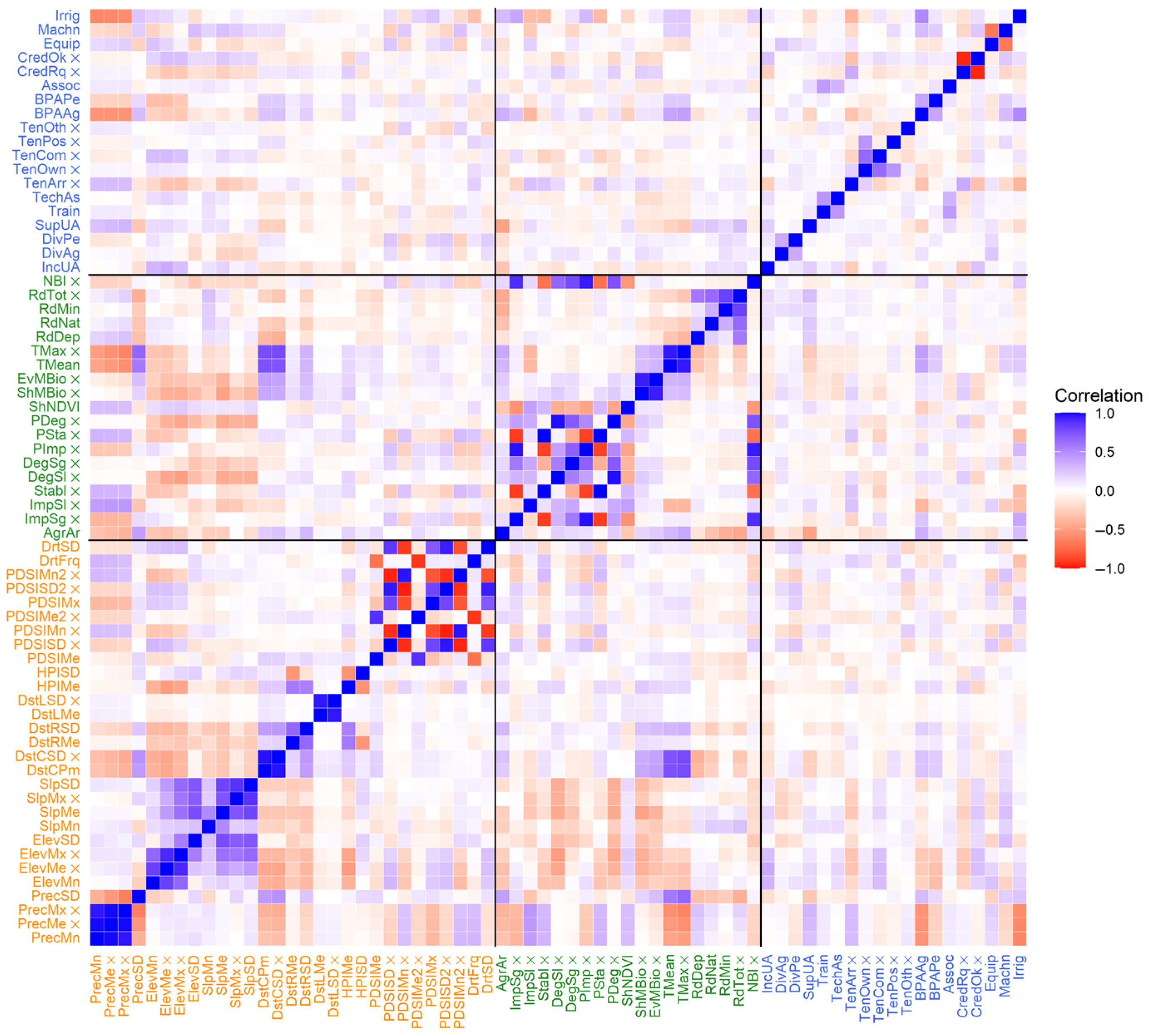
Figure 2 illustrates the correlation structure of the harmonized indicators, grouped by dimension: Environmental Exposure (orange), Ecosystem Condition (green), and Socioeconomic Capacity (blue). Variables marked with an “×” were removed following variance inflation factor (VIF) analysis (threshold > 10) to eliminate redundancy arising from highly collinear indicators and mutually dependent proportions. Overall, the matrix is characterized by predominantly weak to moderate correlations (|r| < 0.5) across dimensions, indicating a high degree of complementarity and limited overlap among the selected indicators. Within dimensions, coherent correlation patterns are observed, reflecting shared underlying processes (e.g., climatic stressors, vegetation dynamics, and socioeconomic capacity). The resulting block-diagonal structure and low inter-dimensional correlations confirm the multidimensional nature of agro-productive and territorial vulnerability and support the use of PCA for dimensional integration and composite index construction.

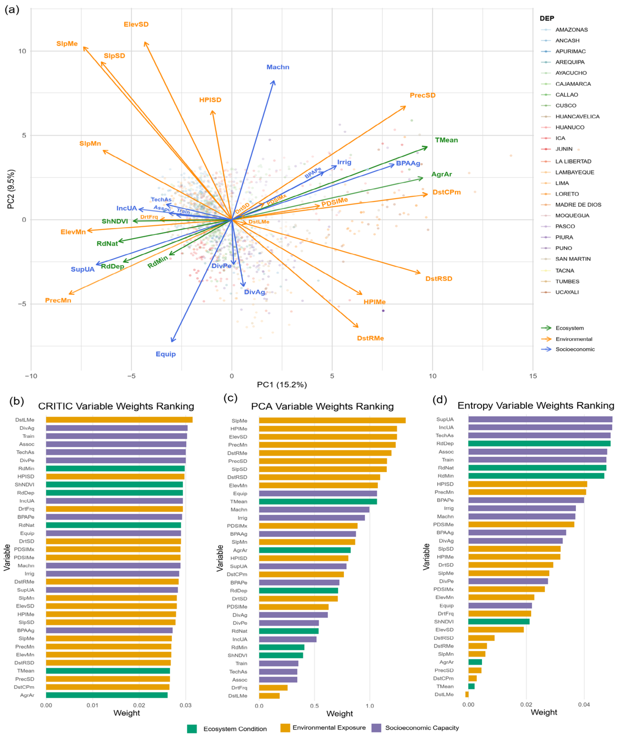
Figure 3 shows the PCA biplot together with the ranking of normalized indicator weights obtained from the CRITIC, PCA and ENTROPY methods. In Figure 3a, the PCA biplot illustrating the multivariate structure of 35 indicators across the first two principal components (PC1: 15.2%; PC2: 9.6%). Vectors represent indicators color-coded by vulnerability dimension: ecosystem condition (green), environmental exposure (orange), and socioeconomic capacity (blue). Vector length indicates contribution magnitude to principal components, while direction reveals inter-indicator relationships. Clustered vectors indicate positive correlations: environmental indicators (PrecMn, PrecSD) align with drought variables (DstRSD, DstLSD) in right quadrants, while terrain complexity indicators (ElevMn, ElevMe, ElevSD, SlpMn, SlpMe, SlpMx, SlpSD) cluster on the left side of PC1, reflecting topographic intercorrelation.

Opposing vectors reveal inverse relationships: precipitation indicators project opposite to elevation and slope metrics along PC1, capturing Peru’s precipitation-elevation gradient. Socioeconomic indicators display dispersed orientations (Machn toward positive PC2, Equip toward negative PC2), with variables like TechAs, Irrig, BPAAg, CredOk, Assoc, Train, SupUA, DivAg, and DivPe pointing in divergent directions, underscoring multidimensional socioeconomic heterogeneity. Points represent Peru’s 25 departments and Callao, revealing substantial territorial variation in precipitation patterns, drought exposure, terrain complexity, and socioeconomic development.

In Figure 3b, CRITIC variable weights ranking derived from the Criteria Importance Through Intercriteria Correlation method, prioritizing indicators with high variability and low intercorrelation. Top-weighted indicators include DstLMe (long-term drought severity mean), DivAg (agricultural diversification), TMean (mean temperature), DivPe (livestock diversification), and TechAs (technical assistance), providing unique, complementary information within the vulnerability framework.

In Figure 3c, PCA variable weights ranking quantifying each indicator’s contribution to total explained variance across principal components. Environmental and ecosystem indicators predominate among top-weighted variables, including SlpMx (maximum slope), HPIMe (hydrological proximity index mean), NBI (unsatisfied basic needs index), PDSIMn (Palmer Drought Severity Index minimum), DstLMe (long-term drought severity mean), ElevMn (mean elevation), and SlpSD (slope standard deviation), reflecting the variance structure revealed in panel a and emphasizing indicators that define the principal axes of territorial differentiation.

In Figure 3d, ENTROPY variable weights ranking calculated through the entropy method, assigning greater weight to indicators with higher information content and dispersion across the dataset. Top-weighted indicators include SupUA (urban area of agricultural units), IncUA (income from urban areas), TechAs (technical assistance), TMean (mean temperature), Assoc (association membership), RdNat (natural road density), and ShNDVI (Shannon diversity of NDVI), effectively discriminating among regions based on distributional heterogeneity.

Together, panels b–d demonstrate how different mathematical formulations (CRITIC: contrast and independence; PCA: variance structure; ENTROPY: information content) emphasize distinct indicator subsets from the multivariate relationships illustrated in panel a.

3.2. Normalized Weights of the Thematic Dimensions

Table 4. Normalized Weights (W_g) of Thematic Dimensions Across Three Weighting Methods.

Dimension	CRITIC	PCA	ENTROPY
Environmental Exposure (EnvExp)	0.407	0.567	0.454
Ecosystem Condition (EcoCond)	0.148	0.141	0.223
Socioeconomic Capacity (SocioCap)	0.445	0.291	0.323

summarizes the normalized weights assigned to the three thematic dimensions under the CRITIC, PCA, and ENTROPY methods. Under CRITIC, SocioCap receives the highest weight (0.445), followed closely by EnvExp (0.407), where variability and indicator conflict emphasize the distinctiveness of social factors. Under PCA and ENTROPY, EnvExp receives the highest weight (0.567 and 0.454, respectively), indicating that climatic and biophysical pressures contribute most strongly to overall vulnerability according to these variance-based and information-theoretic criteria. Ecosystem Condition shows the lowest weights across all methods (0.141–0.223), reflecting its moderate but consistent influence on the vulnerability structure. SocioCap plays a major role, with its weight varying substantially between methods: it is highest under CRITIC (0.445) but comparatively lower under PCA (0.291) and ENTROPY (0.323) due to their different mathematical criteria. Although the three methods differ in magnitude, they show a similar general pattern, with EnvExp and SocioCap emerging as the two dominant dimensions, while EcoCond contributes less. This confirms that vulnerability is jointly shaped by EnvExp, EcoCond, and SocioCap.

3.3. Spatial Distribution of the Vulnerability Sub-Indices

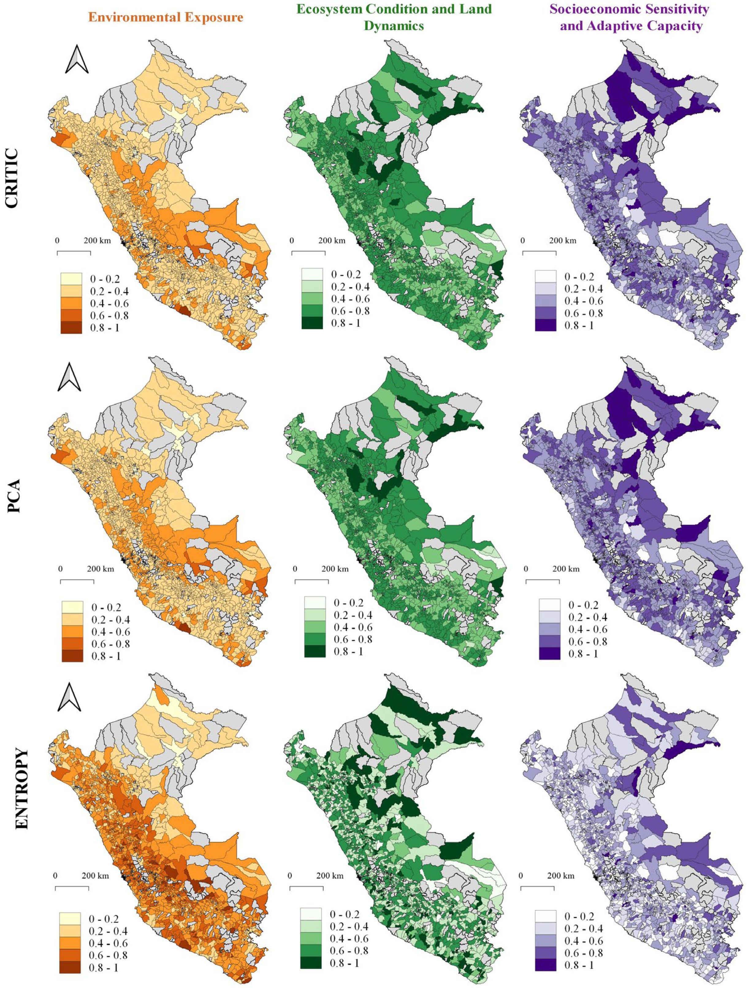
Figure 4 shows the spatial distribution of the three thematic sub-indices derived from the CRITIC, PCA and ENTROPY weighting methods. For Environmental Exposure (EnvExp), the three approaches display similar patterns, with higher values (0.6–1.0) concentrated along the northern and central coastal region (including departments such as Tumbes, Piura, Lambayeque, La Libertad, and Lima), reflecting precipitation variability and drought exposure. In contrast, intermediate to lower values (0.2–0.6) predominate across the Andean highlands (Cusco, Puno, Ayacucho, Huancavelica) and parts of the Amazon Basin (Loreto, Ucayali, Madre de Dios). A clear east–west gradient is evident, with vulnerability decreasing from the arid coast toward the humid Amazon lowlands.

For Ecosystem Condition and Land Dynamics (EcoCond), higher values (0.6–1.0) are observed primarily in the Amazon region (Loreto, Ucayali, Madre de Dios, and San Martín) and parts of the northern Andes (Amazonas, Cajamarca), indicating greater ecosystem pressure from deforestation, land-use change, and agricultural expansion. Conversely, lower values (0–0.4) appear mainly in coastal areas (especially the central and southern coast) and some highland districts, reflecting more stable but potentially degraded vegetation conditions with limited land-cover dynamics. Intermediate values (0.4–0.6) characterize transitional zones in the central highlands.

Regarding Socioeconomic Capacity (SocioCap), the maps show higher values (0.6–1.0) concentrated in districts of the central and southern Andes (Huancavelica, Apurímac, Ayacucho, Puno, and parts of Cusco), where limited infrastructure, lower income, reduced mechanization, and diminished access to technical assistance and credit increase socioeconomic vulnerability. In contrast, lower values (0–0.4) predominate across the coastal strip (particularly near Lima and other urban centers) and extensive areas of the Amazon region (Loreto, Ucayali), where better road connectivity, market access, and resource availability reduce socioeconomic constraints. The spatial pattern reveals a clear core-periphery structure, with the most remote highland districts exhibiting the highest socioeconomic vulnerability.

Although each method (CRITIC, PCA, ENTROPY) applies different weighting schemes based on distinct mathematical criteria, the overall spatial patterns remain remarkably consistent across all three approaches, with only local variations in the magnitude and distribution of the sub-indices. This consistency validates the robustness of the identified spatial vulnerability patterns and confirms that the three dimensions capture complementary but distinct aspects of territorial vulnerability across Peru.

3.4. District-Level Composite Agro-Productive and Territorial Vulnerability Index

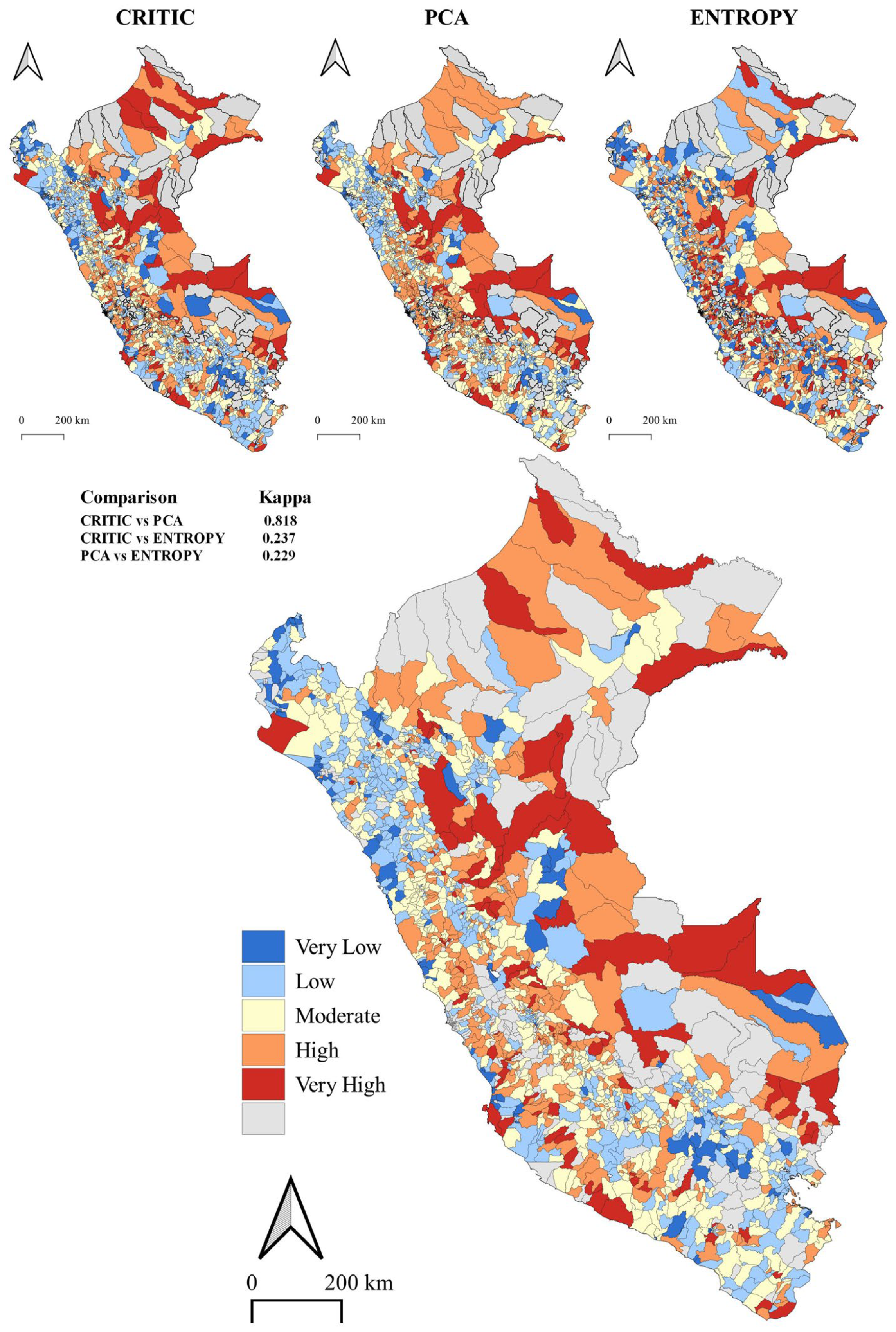
Of the 1891 districts in Peru, 1552 districts were analyzed. Figure 5 presents the district-level vulnerability maps generated using the CRITIC, PCA and ENTROPY methods, together with an integrated modal map that identifies the most frequently occurring vulnerability category across the three approaches for each district.

The three methods produce distinct vulnerability distributions based on their weighting criteria, with varying degrees of district-level agreement as quantified by Cohen’s Kappa statistics. CRITIC and PCA show strong agreement (κ = 0.818), indicating these variance-based approaches classify districts similarly despite different mathematical formulations. However, ENTROPY shows weaker agreement with both CRITIC (κ = 0.237) and PCA (κ = 0.229), reflecting its information-theoretic emphasis on indicator dispersion rather than variance maximization. Despite these methodological differences at the district level, broad spatial patterns remain consistent: vulnerability hotspots emerge in similar geographic zones across all three methods, while disagreements occur primarily in the classification boundaries between adjacent vulnerability categories (e.g., Moderate vs. High).

The modal map reveals the dominant vulnerability pattern by displaying the category that appears in at least two of the three methods for each district. High to Very High vulnerability is consistently identified in portions of the Amazon region (particularly northern Loreto and eastern areas including Ucayali and Madre de Dios), reflecting ecosystem pressures from deforestation, land-use dynamics, and limited infrastructure in remote areas. The central and southern Andean corridor displays a highly heterogeneous mosaic, with some highland districts in Huancavelica, Ayacucho, Apurímac, Junín, and Puno showing High to Very High vulnerability due to the combined effects of terrain complexity, socioeconomic limitations, and environmental exposure, while other Andean districts exhibit Low to Moderate vulnerability where better connectivity and agricultural productivity prevail.

The coastal region presents mixed patterns: the northern coast (Tumbes, Piura, Lambayeque) shows predominantly Moderate to High vulnerability associated with drought exposure and water scarcity, while the central coast near Lima displays lower vulnerability due to superior infrastructure and economic development. The southern coast exhibits variable conditions depending on irrigation availability and local economic activities.

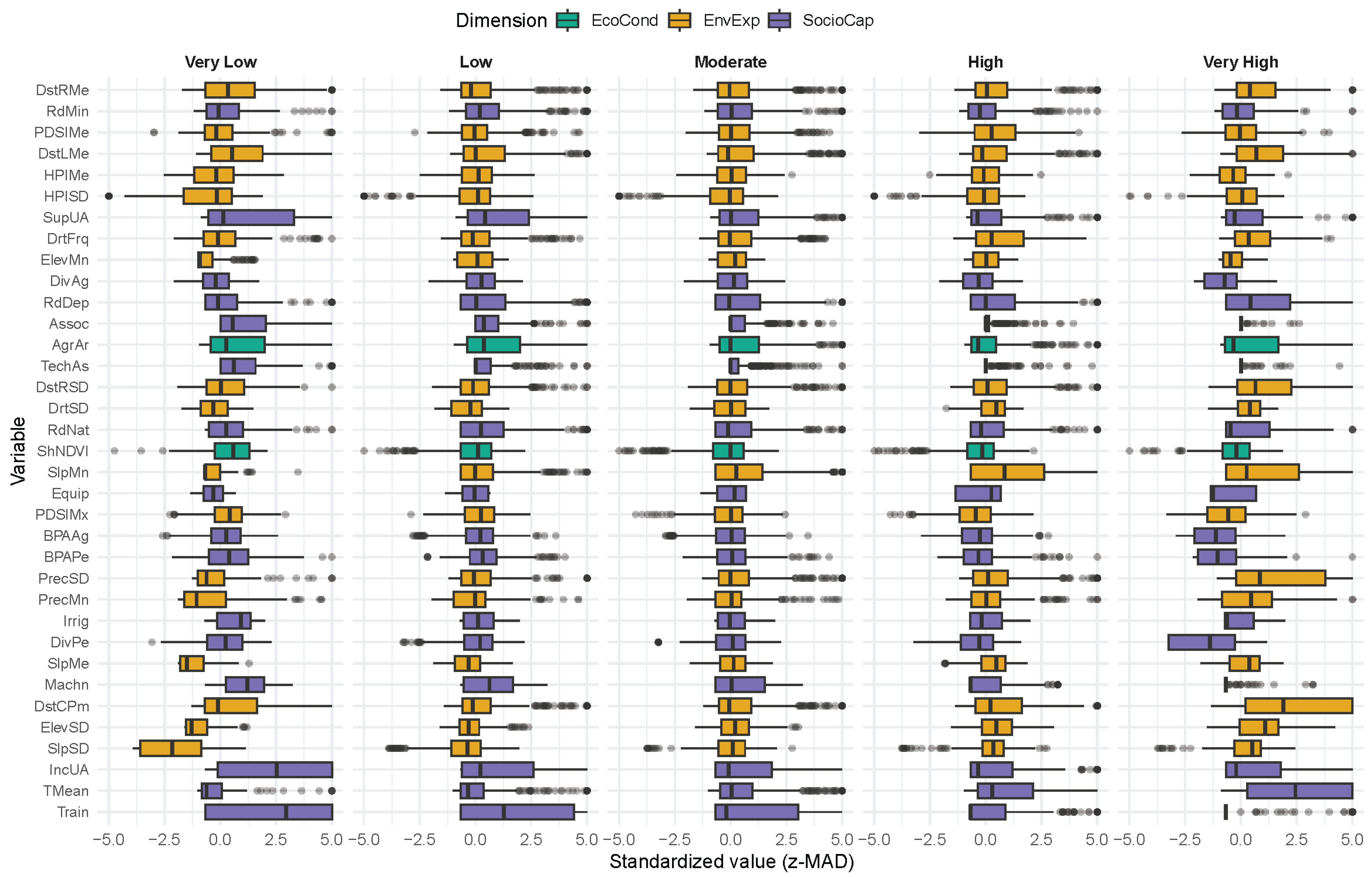
Figure 6 illustrates the distribution of original indicator values (z-MAD standardized) across the five vulnerability classes derived from the composite index. Indicators are organized by thematic dimension: Ecosystem Condition (EcoCond, green), Environmental Exposure (EnvExp, orange), and Socioeconomic Capacity (SocioCap, purple). Z-MAD standardization (median-centered, scaled by median absolute deviation) enables comparison across different units and scales. Positive values indicate above-median conditions; negative values indicate below-median conditions. Interpretation depends on directionality: for cost-type indicators (slope, drought, distance to water), above-median values increase vulnerability; for benefit-type indicators (technical assistance, income, irrigation), above-median values reduce vulnerability.

The figure reveals systematic differences in original territorial conditions across vulnerability classes. Districts classified as Very High vulnerability exhibit positive medians for cost-type environmental indicators—above-average terrain complexity (SlpMn, ElevMn, ElevSD), greater water isolation (DstCPm, DstRMe), higher precipitation variability (PrecSD), and increased drought exposure (PDSIMe, DrtFrq)—alongside negative medians for benefit-type socioeconomic indicators (TechAs, Irrig, IncUA, Train), confirming below-average access to infrastructure and adaptive resources. Conversely, Very Low vulnerability districts show opposite patterns with negative medians for cost-type indicators and less-negative or near-zero values for benefit-type indicators, reflecting more favorable baseline conditions. Moderate vulnerability districts cluster around the national median (z-MAD ≈ 0) across most indicators, representing intermediate or balanced conditions where neither extreme environmental stress nor exceptional socioeconomic deficits predominate.

Within EnvExp (orange), terrain, hydrological, precipitation, and drought variables show progressive gradation from Very Low through Moderate to Very High classes, demonstrating that vulnerable districts face inherently more challenging biophysical conditions. For EcoCond (green), agricultural area (AgrAr) and vegetation dynamics (ShNDVI) show moderate variation, with Moderate classes exhibiting near-median values, while road infrastructure displays clearer differentiation. In SocioCap (purple), highly vulnerable districts systematically exhibit below-median original values for technical assistance, irrigation, income, diversification, mechanization, and training, while Moderate districts show intermediate access to these resources, and Very Low vulnerability districts display stronger socioeconomic capacity. Widening interquartile ranges from Low to Very High classes indicate increasing territorial heterogeneity among more vulnerable districts.

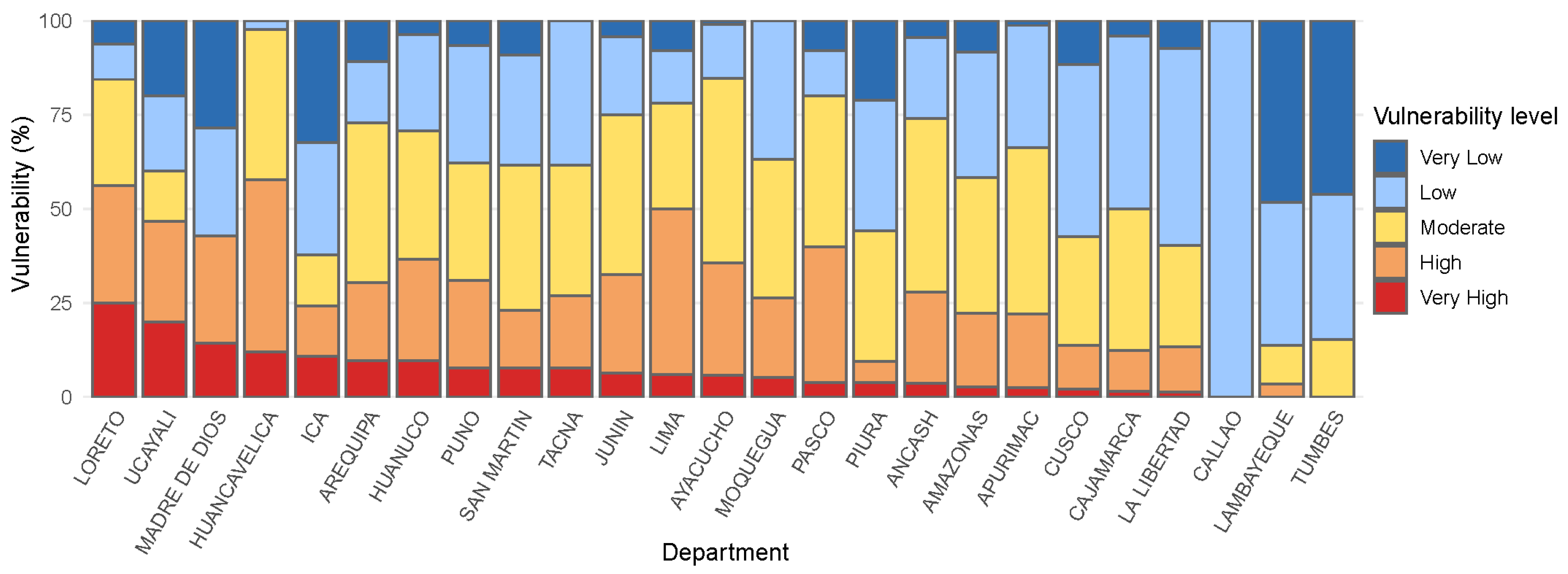
Figure 7 shows the percentage distribution of vulnerability levels (Very Low, Low, Moderate, High, and Very High) at the departmental scale, based on the proportion of districts classified within each category according to the normalized Composite Vulnerability Index. The results reveal pronounced territorial heterogeneity in the internal composition of vulnerability across departments, reflecting marked spatial contrasts in environmental exposure, ecosystem condition, and socioeconomic capacity. Vulnerability patterns do not follow a simple geographic divide but rather reflect complex interactions of biophysical, ecological, and socioeconomic factors.

Departments with highest vulnerability concentrations include Loreto and Ucayali (Amazon), where High and Very High categories together account for 60–70% of districts, with Very High alone reaching ~20–25%. These patterns reflect persistent geographical isolation, limited infrastructure, and elevated environmental pressures. Notably, Ica (southern coast) also exhibits high vulnerability (~70% in High category), likely associated with water scarcity, drought exposure, and irrigation dependence despite coastal location. Huancavelica (central Andes) shows one of the most concentrated High vulnerability patterns (~50–60%), reflecting extreme terrain complexity, limited connectivity, and severe socioeconomic constraints.

Andean and transition departments such as Junín, Pasco, Huánuco, Puno, Ayacucho, and Cusco display heterogeneous distributions, with Moderate and High categories together comprising 50–70% of districts. These departments also present relevant proportions in the Very High category (5–15%), suggesting diverse territorial conditions associated with complex topography, variable accessibility, and mixed agro-productive systems. Madre de Dios shows a balanced distribution with ~45% in High and Very High combined.

Departments with lower vulnerability concentrations include Callao (>90% Very Low/Low), La Libertad (~60% Very Low/Low), and Lambayeque (~55% Very Low/Low), reflecting better urban integration, infrastructure, and economic capacity. However, Lima shows a mixed pattern with only ~30% in Very Low/Low and significant proportions in Moderate and High categories, indicating internal heterogeneity between the metropolitan area and peripheral districts. Tumbes displays ~60% Moderate vulnerability rather than predominantly low levels.

Northern Amazon departments like Amazonas and San Martín exhibit predominantly Moderate to Low vulnerability (~70%), contrasting with the high vulnerability in Loreto and Ucayali, suggesting that Amazon region vulnerability is not uniform but varies substantially by connectivity, land-use intensity, and institutional presence.

4. Discussion

This study demonstrates that territorial vulnerability emerges from the multidimensional interaction between environmental exposure, ecosystem dynamics, and socioeconomic capacity, with their relative importance varying by analytical perspective. The divergence in dimensional weights across methods reveals that CRITIC prioritizes SocioCap due to high heterogeneity across districts, PCA emphasizes EnvExp as the primary variance driver, and ENTROPY balances both dimensions based on information content. Critically, despite divergent dimensional weights and variable rankings, spatial patterns remain consistent across methods, validating the robustness of identified hotspots where multiple stressors converge particularly in Andean-Amazonian transitions and remote highlands.

The spatial complementarity between dimensions reveals critical territorial trade-offs: coastal regions face water scarcity but benefit from infrastructure; Amazon territories experience ecosystem pressure yet lower climatic stress; Andean districts suffer terrain constraints and socioeconomic isolation but maintain stable ecosystems. The progressive differentiation of indicators across vulnerability classes confirms that vulnerability operates through accumulation rather than single-factor dominance, with highly vulnerable districts facing compounding deficits across dimensions. This spatial complexity underscores that vulnerability hotspots do not correspond to simple geographic categories but emerge where environmental challenges compound socioeconomic deficits [70,71].

Methodological diversity in vulnerability assessment from perception-based studies to biophysical assessments [72] to composite indices [41] demonstrates that analytical techniques substantially influence vulnerability estimates. By employing three distinct weighting methods alongside spatial analysis, this study shows that spatial vulnerability patterns remain consistent when multiple dimensions are properly integrated, providing confidence that identified hotspots reflect real territorial conditions rather than methodological artifacts.

4.1. Multivariate Structure of Vulnerability Drivers

The multivariate analysis revealed a coherent internal structure among vulnerability indicators. Correlation matrix and VIF analysis (threshold < 10) showed low collinearity, indicating that environmental, ecosystem, and socioeconomic indicators provide complementary rather than redundant information at the district scale [73].

The PCA biplot captures 24.8% of total variance (PC1: 15.2%, PC2: 9.6%), which reflects Peru’s extreme geographic heterogeneity rather than methodological weakness. Environmental indicators (terrain complexity, hydrological accessibility, precipitation) cluster along PC1, defining a dominant gradient of environmental exposure, while socioeconomic indicators (mechanization, irrigation, credit, technical assistance) display negative loadings and dispersed orientations, reflecting their compensatory role in reducing vulnerability [58]. PC2 contrasts ecosystem degradation indicators (NDVI heterogeneity, land-cover fragmentation) with socioeconomic resilience factors (diversification, income) [74].

Variable weight rankings differ substantially by method based on mathematical formulation: CRITIC emphasizes variables with high variability and low correlation (DstLMx, DivAg, TMean); PCA prioritizes variance contributors (SlpMx, HPIMx, NBI, PDSIMn); ENTROPY weights by information content (SupUA, IncUA, TechAs). Despite these differences, dimensional weights converge in identifying EnvExp and SocioCap as primary drivers, with EcoCond playing a consistent but moderate role (0.141–0.223).

District-level classification agreement, quantified by Cohen’s Kappa, reveals methodological relationships. Strong CRITIC-PCA agreement (κ = 0.818) validates variance-based approaches despite different implementations, while ENTROPY’s weaker agreement (κ = 0.237–0.229) reflects its information-theoretic emphasis on dispersion rather than variance maximization. According to Landis and Koch’s (1977) [75] interpretation guidelines, CRITIC and PCA demonstrate ‘almost perfect agreement’ while ENTROPY shows ‘fair agreement’ with both methods. This divergence is methodologically informative: it demonstrates that classification is sensitive to whether one prioritizes systematic territorial differentiation or local information richness, underscoring the value of multi-method comparison for characterizing classification uncertainty at vulnerability boundaries [76].

These findings confirm that vulnerability does not emerge from a single dominant driver but from the interplay between climatic stressors, ecosystem condition, and socioeconomic capacity [77,78], consistent with previous agro-environmental assessments [42,79]. Integrating multivariate and weighting-based approaches provides more comprehensive representation of agro-territorial systems by reducing redundancy and improving robustness [41]. The combination of high dimensional weight convergence and variable district-level agreement patterns demonstrates that properly integrated multidimensional indices produce stable vulnerability estimates at broad spatial scales while acknowledging methodological sensitivity at classification boundaries.

4.2. Spatial Patterns and Dimensional Complementarity

The spatial distribution of sub-indices reveals striking complementarity between vulnerability dimensions (Figure 4). EnvExp concentrates along the northern and central coast, reflecting precipitation variability, drought exposure, and water scarcity. EcoCond peaks in the Amazon region and northern Andes, indicating ecosystem pressure from deforestation and land-use change [80]. SocioCap shows highest values in the central and southern Andes, where limited infrastructure and reduced access to services compound vulnerability [81].

This dimensional complementarity explains why composite vulnerability hotspots do not correspond to single geographic categories. The modal map (Figure 5) identifies convergence zones where multiple stressors compound: Andean-Amazonian transitions face combined terrain constraints, ecosystem pressure, and socioeconomic isolation; remote highlands experience extreme topography and institutional marginalization; specific coastal areas suffer water scarcity despite connectivity. Conversely, low-vulnerability territories benefit from compensatory mechanisms coastal regions offset environmental stress with infrastructure, while some Amazon districts maintain ecosystem stability despite limited economic development.

Departmental analysis (Figure 7) reveals heterogeneous distributions within administrative boundaries. Amazon departments diverge substantially: Loreto and Ucayali concentrate 60–70% of districts in High/Very High categories, while Amazonas and San Martín show predominantly Moderate/Low vulnerability [82]. Andean departments display internal mosaics, with Huancavelica exhibiting 50–60% High vulnerability. Coastal heterogeneity ranges from Callao’s > 90% Very Low/Low to Ica’s 70% High vulnerability from drought.

Within EcoCond, vegetation diversity (Shannon NDVI, land-cover heterogeneity) shows complex patterns, with higher diversity maintaining ecological stability [81] and simplified landscapes exhibiting degradation susceptibility [83]. However, ecosystem condition emerged as a consistent but moderate contributor (weights: 0.141–0.223), suggesting biophysical exposure and socioeconomic constraints are more powerful differentiators [84].

The spatial consistency across CRITIC, PCA, and ENTROPY methods despite divergent weighting validates that identified patterns reflect real territorial conditions and confirms properly integrated multidimensional assessments are robust to weighting variations. Spatial complementarity underscores that effective vulnerability reduction requires dimension-specific interventions: water infrastructure for coastal EnvExp, ecosystem restoration for Amazon EcoCond, and infrastructure development for Andean SocioCap [81,82].

4.3. Socioeconomic Capacity as Vulnerability Moderator

The z-MAD standardization (Figure 6) demonstrates that socioeconomic capacity functions as a critical vulnerability moderator through systematic differentiation of adaptive resources. Districts classified as Very High vulnerability exhibit consistently negative standardized values for benefit-type indicators like technical assistance (TechAs), irrigation (Irrig), income (IncUA), mechanization (Machn), training (Train), and diversification (DivAg, DivPe) indicating below-median access to adaptive resources. Conversely, Very Low vulnerability districts display less-negative or near-zero values, confirming stronger baseline capacity. This demonstrates that vulnerability emerges from compounding effects: highly vulnerable territories face both biophysical challenges and systematic socioeconomic constraints [85,86].

The progressive widening of interquartile ranges in High and Very High classes reveals increasing heterogeneity, suggesting extreme vulnerability has multiple pathways: some districts are constrained by institutional isolation (low technical assistance), others by productive limitations (low income, minimal mechanization), and others by infrastructure deficits (restricted irrigation, poor credit access). Empirical evidence confirms that access to credit, extension services, and education significantly increases adoption of adaptation practices [87,88], with socioeconomic factors explaining substantial variability in adaptation decisions [89].

Spatial patterns (Figure 4) confirm SocioCap concentrates in the central and southern Andes (Huancavelica, Apurímac, Ayacucho, Puno), where remoteness restricts adaptive resources despite pressing environmental challenges [90,91]. The compensatory role of socioeconomic resources is evident in coastal regions, where connectivity and service access offset environmental stress from drought.

These findings indicate that strengthening adaptive capacity requires coordinated interventions: expanding technical assistance networks in remote highlands, improving credit access for smallholders, investing in irrigation infrastructure in water-scarce regions, and promoting mechanization where viable [15,92,93]. Enhancing adaptive capacity through targeted socioeconomic development constitutes a primary pathway for vulnerability reduction in territories where environmental constraints are difficult to modify [94]

4.4. Implications for Territorial Policy and Sustainable Development

The IVAPT provides an evidence-based framework for differentiated territorial interventions by revealing that vulnerability emerges from dimension-specific processes requiring tailored policy responses. The spatial complementarity between dimensions (Figure 4) demonstrates that effective vulnerability reduction cannot follow a one-size-fits-all approach but must address distinct territorial challenges: water infrastructure and drought management for coastal EnvExp hotspots (Tumbes, Piura, Ica); ecosystem restoration and sustainable land-use planning for Amazon EcoCond pressure zones (Loreto, Ucayali, Madre de Dios); and infrastructure development, technical assistance expansion, and institutional strengthening for Andean SocioCap constraints (Huancavelica, Apurímac, Ayacucho, Puno) [95,96].

Departmental heterogeneity (Figure 7) further refines policy targeting by revealing internal variation within administrative boundaries. Loreto’s 60–70% High/Very High concentration demands prioritized intervention, while Amazonas’ predominantly Moderate/Low profile suggests different needs. Lima’s mixed pattern indicates that metropolitan integration does not automatically reduce vulnerability in peripheral districts, requiring sub-regional differentiation. The modal map (Figure 5) identifies convergence zones where multiple stressors compound Andean-Amazonian transitions, remote highlands as critical intervention priorities where coordinated multi-sectoral approaches yield highest returns [80,97].

The methodological convergence across CRITIC, PCA, and ENTROPY provides policy confidence: identified hotspots reflect real territorial conditions rather than methodological artifacts, enabling robust resource allocation decisions. The integration of census-based socioeconomic indicators with satellite-derived environmental data, leveraging GEE as a freely accessible spatial data repository, creates a transparent, replicable, and cost-effective framework for monitoring vulnerability changes and evaluating intervention effectiveness [98,99].

The IVAPT advances SDG 2 (Zero Hunger), SDG 6 (Clean Water), SDG 13 (Climate Action), and SDG 15 (Life on Land) by identifying where interventions provide greatest benefits for food security, water management, and ecosystem restoration [41,81]. Its replicable structure enables scaling to other Andean countries, supporting regional adaptation frameworks [100]. Beyond analytical value, the IVAPT serves as a governance instrument promoting cross-sectoral coordination between environmental agencies, agricultural ministries, and rural development programs, enhancing institutional efficiency and resource allocation to high-risk rural areas [101].

4.5. Limitations and Future Research

The IVAPT faces primarily data-related limitations. Temporal constraints limit dynamic monitoring: the agricultural census provides comprehensive district-level coverage but reflects a single time point (2012), restricting ability to track vulnerability trajectories. While the National Agricultural Survey (ENA) offers the most temporally current annual data, its current sample size would need to be substantially increased to enable robust district-level disaggregation. Despite this limitation, ENA remains the best available source for monitoring temporal trends, suggesting future research should explore hybrid approaches that combine census spatial baselines with ENA temporal patterns at aggregated scales (provincial/departmental) or advocate for ENA sample expansion to enable finer spatial resolution [102]. Spatial resolution limitations challenge smallholder representation: 30 m Landsat imagery may inadequately capture agricultural mosaics in highly fragmented Andean landscapes where plots are often <1 hectare [103]. Aggregation scale masks heterogeneity: widening interquartile ranges (Figure 6) suggest district-level aggregation conceals sub-district variation. Administrative boundaries misalign with vulnerability patterns (Figure 7): departmental units constrain policy implementation yet do not correspond to vulnerability hotspots.

Future efforts should: (1) integrate higher-resolution imagery (Sentinel-2 10 m, PlanetScope 3 m) for better smallholder representation [104]; (2) develop census-ENA hybrid frameworks leveraging ENA’s temporal continuity while advocating for sample expansion; (3) incorporate dynamic socio-ecological variables (water infrastructure, migration, technology adoption); (4) develop sub-district vulnerability mapping for heterogeneous areas; (5) apply machine learning to identify non-linear interactions [105]; and (6) implement participatory validation with local stakeholders.

5. Conclusions

This study demonstrates that agro-productive and territorial vulnerability in Peru emerges from multidimensional interactions between environmental exposure, ecosystem dynamics, and socioeconomic capacity, with spatial patterns reflecting their complementary rather than uniform distribution. The IVAPT revealed that highest vulnerability concentrates primarily in the Amazon region (Loreto, Ucayali, Madre de Dios), Andean-Amazonian transitions, and specific highland districts (Huancavelica, Apurímac, Ayacucho, Puno) where biophysical constraints, ecosystem pressure, and socioeconomic isolation converge. Dimensional complementarity EnvExp peaking on the coast, EcoCond in the Amazon, SocioCap in the Andes underscores that effective vulnerability reduction requires dimension-specific interventions rather than uniform policies. The methodological convergence across CRITIC, PCA, and ENTROPY despite divergent weighting schemes validates the robustness of identified hotspots. Leveraging Google Earth Engine as a freely accessible spatial data repository, the IVAPT provides a transparent, replicable framework for evidence-based territorial planning that supports priority targeting of investments in water infrastructure, ecosystem restoration, and institutional strengthening. Addressing identified limitations particularly temporal monitoring constraints, spatial resolution gaps, and aggregation scale mismatches requires coordinated advances in data infrastructure, analytical methods, and participatory validation. An updated, georeferenced agricultural census built on contemporary geospatial standards would substantially strengthen the evidence base for targeted territorial interventions essential for climate adaptation and sustainable rural development.

References

1. Sun, J.; Hua, E.; Sun, S.; Yin, Y.; Wang, Y.; Zhao, J.; Tang, Y.; Wu, P. Sustainability Assessment of Agricultural Development in China: Water-Carbon Footprint Perspective. Agric. Water Manag. 2025, 320, 109835. [Google Scholar] [CrossRef]
2. Sharma, V.; Kaur, G.; Chhabra, V.; Kashyap, R. Smart Irrigation Systems in Agriculture: An Overview. Comput. Electron. Agric. 2025, 239, 111008. [Google Scholar] [CrossRef]
3. Omotayo, A.O.; Adeoye, A.; Omotoso, A.B.; Ogunniyi, A.I. Impact of Conflicts on Agricultural Crop Investment in Rural Areas: Policy Insight from a Nationally Representative Survey Dataset. Land Use Policy 2025, 159, 107793. [Google Scholar] [CrossRef]
4. Zeleke, E.B.; Mohammed, M.; Kidanewold, B.B. Vulnerability Assessment of Smallholder Farmers to Climate Change in the Awash Basin, Ethiopia. Environ. Sustain. Indic. 2025, 28, 100927. [Google Scholar] [CrossRef]
5. Tanir, T.; Yildirim, E.; Ferreira, C.M.; Demir, I. Social Vulnerability and Climate Risk Assessment for Agricultural Communities in the United States. Sci. Total Environ. 2024, 908, 168346. [Google Scholar] [CrossRef]
6. Alam, A.; Banna, H.; Roni, N.N.; Abedin, M.Z. Sowing Sustainability: How Does Fintech Mitigate Agricultural Financial Risk from Climate Change Vulnerability. Int. Rev. Econ. Financ. 2025, 101, 104226. [Google Scholar] [CrossRef]
7. Habtie, T.T.; Teferi, E.; Guta, F. Spatiotemporal Patterns of Socioecological Vulnerability in Tigray, Ethiopia: A Multi-Level Analysis of Climate and Land-Use Change Impacts on Agricultural Households. Sci. Afr. 2025, 30, e02982. [Google Scholar] [CrossRef]
8. Lia, Y.; Gao, G.; Wen, J.; Zhao, N.; Du, G.; Stanny, M. The Measurement of Agricultural Disaster Vulnerability in China and Implications for Land-Supported Agricultural Resilience Building. Land Use Policy 2025, 148, 107400. [Google Scholar] [CrossRef]
9. Motha, R.P.; Baier, W. Impacts of Present and Future Climate Change and Climate Variability on Agriculture in the Temperate Regions: North America. Clim. Change 2005, 70, 137–164. [Google Scholar] [CrossRef]
10. Fanzo, J. From Big to Small: The Significance of Smallholder Farms in the Global Food System. Lancet Planet. Health 2017, 1, e15–e16. [Google Scholar] [CrossRef]
11. Cheng, W.; Li, Y.; Zuo, W.; Du, G.; Stanny, M. Spatio-Temporal Detection of Agricultural Disaster Vulnerability in the World and Implications for Developing Climate-Resilient Agriculture. Sci. Total Environ. 2024, 928, 172412. [Google Scholar] [CrossRef] [PubMed]
12. Gollin, D. Agricultural Productivity and Structural Transformation: Evidence and Questions for African Development. Oxf. Dev. Stud. 2023, 51, 375–396. [Google Scholar] [CrossRef]
13. Yogi, L.N.; Thalal, T.; Bhandari, S. The Role of Agriculture in Nepal’s Economic Development: Challenges, Opportunities, and Pathways for Modernization. Heliyon 2025, 11, e41860. [Google Scholar] [CrossRef] [PubMed]
14. Chen, F.; Jia, H.; Du, E.; Chen, Y.; Wang, L. Modeling of the Cascading Impacts of Drought and Forest Fire Based on a Bayesian Network. Int. J. Disaster Risk Reduct. 2024, 111, 104716. [Google Scholar] [CrossRef]
15. FAO. IFAD United Nations Decade of Family Farming 2019–2028 Global Action Plan; FAO: Rome, Italy, 2019; ISBN 9789251314722. [Google Scholar]
16. Dieguez, H.; Gallego, F.; Camba Sans, G.; Staiano, L.; Baldassini, P.; Ruggia, A.; Aguerre, V.; Paruelo, J.M. Family Farming Stands out for Its Environmental Performance in Uruguay’s Agricultural Sector. Agric. Syst. 2025, 229, 104440. [Google Scholar] [CrossRef]
17. Barrientos Felipa, P. La Agricultura Peruana y Su Capacidad de Competir En El Mercado Internacional. Equidad Desarro. 2018, 32, 143–179. [Google Scholar] [CrossRef]
18. Ccopi, D.; Ortega, K.; Castañeda, I.; Rios, C.; Enriquez, L.; Patricio, S.; Ore, Z.; Casanova, D.; Agurto, A.; Zuñiga, N.; et al. Using UAV Images and Phenotypic Traits to Predict Potato Morphology and Yield in Peru. Agriculture 2024, 14, 1876. [Google Scholar] [CrossRef]
19. Aguilar-Luis, M.A.; Sanchez, J.M.; Mercado, W.; Alegre, J.C. Sustainable Agriculture in Peru Based on Agrobiodiversity and Climate-Smart Agriculture: Evaluation of a Case Study with Small Farmers in an Andean Basin. J. Ecol. Eng. 2024, 25, 278–293. [Google Scholar] [CrossRef]
20. FAO. La Agricultura Familiar en el Perú; Organización de las Naciones Unidas para la Alimentación y la Agricultura: Roma, Italy, 2023. [Google Scholar]
21. MIDAGRI. Estrategia Nacional de Agricultura Familiar 2015–2021; MIDAGRI: Lima, Peru, 2014. [Google Scholar]
22. INEI. Productores Agropecuarios—Principales Resultados de La Encuesta Nacional Agropecuaria (ENA); Instituto Nacional de Estadistica e Informatica: Lima, Peru, 2023. [Google Scholar]
23. INEI. La Agricultura Familiar En El Perú: Retos y Posibilidades Para Su Transformación En El Contexto de Los Objetivos de Desarrollo Sostenible (ODS); INEI: Lima, Peru, 2024. [Google Scholar]
24. Mortensen, E.; Block, P. ENSO Index-Based Insurance for Agricultural Protection in Southern Peru. Geosciences 2018, 8, 64. [Google Scholar] [CrossRef]
25. Gubler, S.; Rossa, A.; Avalos, G.; Brönnimann, S.; Cristobal, K.; Croci-Maspoli, M.; Dapozzo, M.; van der Elst, A.; Escajadillo, Y.; Flubacher, M.; et al. Twinning SENAMHI and MeteoSwiss to Co-Develop Climate Services for the Agricultural Sector in Peru. Clim. Serv. 2020, 20, 100195. [Google Scholar] [CrossRef]
26. MIDAGRI. Mapa Nacional de Superficie Agrícola Del Perú; MIDAGRI: Lima, Peru, 2025. [Google Scholar]
27. Heikkinen, A.M. Climate Change, Power, and Vulnerabilities in the Peruvian Highlands. Reg. Environ. Change 2021, 21, 82. [Google Scholar] [CrossRef]
28. Coayla, E.; Culqui, E. Vulnerability Assessment and Adaptation Costs of Agriculture to Climate Change in the Lima Region, Peru. Int. J. Environ. Sci. Dev. 2020, 11, 26–35. [Google Scholar] [CrossRef][Green Version]
29. García, L.; Veneros, J.; Oliva-Cruz, M.; Olivares, N.; Chavez, S.G.; Rojas-Briceño, N.B. Construction of Linear Models for the Normalized Vegetation Index (NDVI) for Coffee Crops in Peru Based on Historical Atmospheric Variables from the Climate Engine Platform. Atmosphere 2024, 15, 923. [Google Scholar] [CrossRef]
30. Vieira, M.T.; Vieira, A.V.; García, C.M.V. Vulnerability Index Elaboration for Climate Change Adaptation in Peru. Eur. J. Sustain. Dev. 2019, 8, 102. [Google Scholar] [CrossRef]
31. Senamhi BOLETÍN AGRO. Hidroclimático Mensual; Senamhi BOLETÍN AGRO: Lima, Peru, 2022. [Google Scholar]
32. Zegarra, E.; Vásquez, Y. Las Múltiples Crisis de La Agricultura Familiar En Perú Entre 2020 y 2023; Friedrich-Ebert-Stiftung Ecuador FES-ILDIS: Quito, Ecuador, 2025. [Google Scholar]
33. FAO. Promoting the Development of Family Farming in Peru; FAO: Rome, Italy, 2023. [Google Scholar]
34. INEI. Encuesta Nacional Agropecuaria (ENA) 2024—[Instituto Nacional de Estadística e Informática—INEI]. Available online: https://proyectos.inei.gob.pe/microdatos/Consulta_por_Encuesta.asp (accessed on 15 October 2025).
35. USGS. Landsat 7, 8, and 9 Surface Reflectance Tier 1 Products (Collection 2) [Data Set]. Earth Resources Observation and Science (EROS) Center. Available online: https://www.usgs.gov/landsat-missions (accessed on 15 October 2025).
36. Gorelick, N.; Hancher, M.; Dixon, M.; Ilyushchenko, S.; Thau, D.; Moore, R. Google Earth Engine: Planetary-Scale Geospatial Analysis for Everyone. Remote Sens. Environ. 2017, 202, 18–27. [Google Scholar] [CrossRef]
37. Weiss, D.J.; Nelson, A.; Gibson, H.S.; Temperley, W.; Peedell, S.; Lieber, A.; Hancher, M.; Poyart, E.; Belchior, S.; Fullman, N.; et al. A Global Map of Travel Time to Cities to Assess Inequalities in Accessibility in 2015. Nature 2018, 553, 333–336. [Google Scholar] [CrossRef]
38. NASA. USGS Shuttle Radar Topography Mission (SRTM) 1 Arc-Second Global [Data Set]. NASA EOSDIS Land Processes DAAC. Available online: https://www.earthdata.nasa.gov/data/catalog/lpcloud-srtmgl1-003 (accessed on 15 October 2025).
39. ANA. Infraestructura Hídrica y Cuerpos de Agua Del Perú. Available online: https://www.gob.pe/ana (accessed on 15 October 2025).
40. MapBiomas Cobertura y Uso Del Suelo de Perú—Colección 3. Available online: https://peru.mapbiomas.org/ (accessed on 15 October 2025).
41. Wiréhn, L.; Danielsson, Å.; Neset, T.-S.S. Assessment of Composite Index Methods for Agricultural Vulnerability to Climate Change. J. Environ. Manag. 2015, 156, 70–80. [Google Scholar] [CrossRef]
42. Loi, D.T.; Van Huong, L.; Tuan, P.A.; Nhung, N.T.H.; Huong, T.T.Q.; Man, B.T.H. An Assessment of Agricultural Vulnerability in the Context of Global Climate Change: A Case Study in Ha Tinh Province, Vietnam. Sustainability 2022, 14, 1282. [Google Scholar] [CrossRef]
43. Cortés, J.; Vieli, L.; Ibarra, J.T. Family Farming Systems: An Index-Based Approach to the Drivers of Agroecological Principles in the Southern Andes. Ecol. Indic. 2023, 154, 110640. [Google Scholar] [CrossRef]
44. Moreira, L.L.; Vanelli, F.M.; Schwamback, D.; Kobiyama, M.; de Brito, M.M. Sensitivity Analysis of Indicator Weights for the Construction of Flood Vulnerability Indexes: A Participatory Approach. Front. Water 2023, 5, 970469. [Google Scholar] [CrossRef]
45. Zhang, X.; Wang, C.; Li, E.; Xu, C. Assessment Model of Ecoenvironmental Vulnerability Based on Improved Entropy Weight Method. Sci. World J. 2014, 2014, 797814. [Google Scholar] [CrossRef]
46. Sarker, S.; Jahan, I.; Wang, X.; Azad, A. Geospatial Approach to Assess Flash Flood Vulnerability in a Coastal District of Bangladesh: Integrating the Multifaceted Dimension of Vulnerabilities. ISPRS Int. J. Geoinf. 2025, 14, 194. [Google Scholar] [CrossRef]
47. Liu, Y.; Zheng, J.; Lu, H.; Li, X. Vulnerability Assessment and Spatio-Temporal Dynamics Analysis of Agricultural Flood in China. Front. Environ. Sci. 2022, 10, 902968. [Google Scholar] [CrossRef]
48. Wang, T.-C.; Lee, H.-D. Developing a Fuzzy TOPSIS Approach Based on Subjective Weights and Objective Weights. Expert. Syst. Appl. 2009, 36, 8980–8985. [Google Scholar] [CrossRef]
49. ZOU, Z.; YUN, Y.; SUN, J. Entropy Method for Determination of Weight of Evaluating Indicators in Fuzzy Synthetic Evaluation for Water Quality Assessment. J. Environ. Sci. 2006, 18, 1020–1023. [Google Scholar] [CrossRef]
50. Wang, B.; Teng, Y.; Wang, H.; Zuo, R.; Zhai, Y.; Yue, W.; Yang, J. Entropy Weight Method Coupled with an Improved DRASTIC Model to Evaluate the Special Vulnerability of Groundwater in Songnen Plain, Northeastern China. Hydrol. Res. 2020, 51, 1184–1200. [Google Scholar] [CrossRef]
51. Zhu, H.; Yao, J.; Meng, J.; Cui, C.; Wang, M.; Yang, R. A Method to Construct an Environmental Vulnerability Model Based on Multi-Source Data to Evaluate the Hazard of Short-Term Precipitation-Induced Flooding. Remote Sens. 2023, 15, 1609. [Google Scholar] [CrossRef]
52. Yang, X.; Zhou, X.; Shang, G.; Zhang, A. An Evaluation on Farmland Ecological Service in Jianghan Plain, China --from Farmers’ Heterogeneous Preference Perspective. Ecol. Indic. 2022, 136, 108665. [Google Scholar] [CrossRef]
53. Diakoulaki, D.; Mavrotas, G.; Papayannakis, L. Determining Objective Weights in Multiple Criteria Problems: The Critic Method. Comput. Oper. Res. 1995, 22, 763–770. [Google Scholar] [CrossRef]
54. Zhang, Y.; Ding, C.; Liu, Y.; Li, S.; Li, X.; Xi, B.; Duan, J. Xylem Anatomical and Hydraulic Traits Vary within Crown but Not Respond to Water and Nitrogen Addition in Populus Tomentosa. Agric. Water Manag. 2023, 278, 108169. [Google Scholar] [CrossRef]
55. Jolliffe, I.T.; Cadima, J. Principal Component Analysis: A Review and Recent Developments. Philos. Trans. R. Soc. A Math. Phys. Eng. Sci. 2016, 374, 20150202. [Google Scholar] [CrossRef]
56. Abson, D.J.; Dougill, A.J.; Stringer, L.C. Using Principal Component Analysis for Information-Rich Socio-Ecological Vulnerability Mapping in Southern Africa. Appl. Geogr. 2012, 35, 515–524. [Google Scholar] [CrossRef]
57. Rao, S.-H. Transportation Synthetic Sustainability Indices: A Case of Taiwan Intercity Railway Transport. Ecol. Indic. 2021, 127, 107753. [Google Scholar] [CrossRef]
58. Medina, N.; Abebe, Y.A.; Sanchez, A.; Vojinovic, Z. Assessing Socioeconomic Vulnerability after a Hurricane: A Combined Use of an Index-Based Approach and Principal Components Analysis. Sustainability 2020, 12, 1452. [Google Scholar] [CrossRef]
59. Sruthi Krishnan, V.; Mohammed Firoz, C. Regional Urban Environmental Quality Assessment and Spatial Analysis. J. Urban Manag. 2020, 9, 191–204. [Google Scholar] [CrossRef]
60. Jenks, F. The Data Model Concept in Statistical Mapping; University of KansasKenneth Spencer Research Library: Lawrence, KS, USA, 1967. [Google Scholar]
61. Saleh, M. Evaluation of Jenks Natural Breaks Clustering Algorithm for Changepoint Identification in Streaming Sensor Data. IEEE Sens. Lett. 2024, 8, 1–4. [Google Scholar] [CrossRef]
62. R Core Team. R: A Language and Environment for Statistical Computing; R Core Team: Vienna, Austria, 2024. [Google Scholar]
63. Wickham, H.; François, R.; Henry, L.; Müller, K.; Vaughan, D. Dplyr: A Grammar of Data Manipulation. CRAN: Contributed Packages; Posit Software, PBC: Boston, MA, USA, 2014. [Google Scholar]
64. Pebesma, E. Sf: Simple Features for R. CRAN: Contributed Packages; Posit Software, PBC: Boston, MA, USA, 2016. [Google Scholar]
65. Hijmans, R.J. Terra: Spatial Data Analysis. CRAN: Contributed Packages; Posit Software, PBC: Boston, MA, USA, 2020. [Google Scholar]
66. Lê, S.; Josse, J.; Rennes, A.; Husson, F. FactoMineR: An R Package for Multivariate Analysis. J. Stat. Softw. 2008, 25, 1–18. [Google Scholar] [CrossRef]
67. Kassambara, A.; Mundt, F. Factoextra: Extract and Visualize the Results of Multivariate Data Analyses. CRAN: Contributed Packages; Posit Software, PBC: Boston, MA, USA, 2016. [Google Scholar]
68. Fox, J.; Weisberg, S.; Price, B. Car: Companion to Applied Regression. CRAN: Contributed Packages; Posit Software, PBC: Boston, MA, USA, 2001. [Google Scholar]
69. Rousseeuw, P.J.; Croux, C. Alternatives to the Median Absolute Deviation. J. Am. Stat. Assoc. 1993, 88, 1273–1283. [Google Scholar] [CrossRef]
70. Abid, M.; Scheffran, J.; Schneider, U.A.; Ashfaq, M. Farmers’ Perceptions of and Adaptation Strategies to Climate Change and Their Determinants: The Case of Punjab Province, Pakistan. Earth Syst. Dyn. 2015, 6, 225–243. [Google Scholar] [CrossRef]
71. Uddin, M.; Bokelmann, W.; Entsminger, J. Factors Affecting Farmers’ Adaptation Strategies to Environmental Degradation and Climate Change Effects: A Farm Level Study in Bangladesh. Climate 2014, 2, 223–241. [Google Scholar] [CrossRef]
72. Nguyen, T.; Mula, L.; Cortignani, R.; Seddaiu, G.; Dono, G.; Virdis, S.; Pasqui, M.; Roggero, P. Perceptions of Present and Future Climate Change Impacts on Water Availability for Agricultural Systems in the Western Mediterranean Region. Water 2016, 8, 523. [Google Scholar] [CrossRef]
73. Mutunga, E.J.; Ndungu, C.K.; Mwangi, M.; Kariuki, P.C. Socioeconomic Determinants of Farmers’ Vulnerability to Climate Variability and Extreme Events in Kitui County, Kenya. Am. J. Clim. Change 2024, 13, 647–663. [Google Scholar] [CrossRef]
74. Raju, K.V.; Deshpande, R.S.; Bedamatta, S. Vulnerability to Climate Change: A Sub-Regional Analysis of Socio-Economic and Agriculture Sectors in Karnataka, India. J. Dev. Policy Pract. 2017, 2, 24–55. [Google Scholar] [CrossRef]
75. Landis, J.R.; Koch, G.C. The Measurement of Observer Agreement for Categorical Data. Biometrics 1977, 33, 159–174. [Google Scholar] [CrossRef] [PubMed]
76. Wu, R.M.X.; Zhang, Z.; Yan, W.; Fan, J.; Gou, J.; Liu, B.; Gide, E.; Soar, J.; Shen, B.; Fazal-e-Hasan, S.; et al. A comparative analysis of the principal component analysis and entropy weight methods to establish the indexing measurement. PLoS ONE 2022, 17, e0262261, Erratum in PLoS ONE 2024, 19, e0314513. https://doi.org/10.1371/journal.pone.0314513. [Google Scholar] [CrossRef]
77. Duvil, J.; Feuillet, T.; Emmanuel, E.; Paul, B. Assessing the Vulnerability of Farming Households on the Caribbean Island of Hispaniola to Climate Change. Climate 2024, 12, 138. [Google Scholar] [CrossRef]
78. Zaatra, A.; Requier-Desjardins, M.; Rey-Valette, H.; Blayac, T.; Belhouchette, H. Assessment of Farm Vulnerability to Climate Change in Southern France. Land 2025, 14, 1388. [Google Scholar] [CrossRef]
79. Janani, H.K.; Karunanayake, C.; Gunathilake, M.B.; Rathnayake, U. Integrating Indicators in Agricultural Vulnerability Assessment to Climate Change. Agric. Res. 2024, 13, 741–754. [Google Scholar] [CrossRef]
80. Raza, A.; Syed, N.R.; Fahmeed, R.; Acharki, S.; Aljohani, T.H.; Hussain, S.; Zubair, M.; Zahra, S.M.; Islam, A.R.M.T.; Almohamad, H.; et al. Investigation of Changes in Land Use/Land Cover Using Principal Component Analysis and Supervised Classification from Operational Land Imager Satellite Data: A Case Study of under Developed Regions, Pakistan. Discov. Sustain. 2024, 5, 73. [Google Scholar] [CrossRef]
81. Tárníková, M.; Muchová, Z. Ecological Stability over the Period: Land-Use Land-Cover Change and Prediction for 2030. Land 2025, 14, 1503. [Google Scholar] [CrossRef]
82. Wang, S.; Song, Q.; Tang, M.; Zhang, H.; Lu, Z. Landscape Ecological Risk Evaluation Coupled with Ecosystem Service Improvement and Its Spatial Heterogeneity Analysis: A Case Study of the Yellow River Source Area. Geomat. Nat. Hazards Risk 2024, 15, 2396895. [Google Scholar] [CrossRef]
83. Makwinja, R.; Curtis, C.J.; Tesfamichael, S.G. Vulnerability of Ecosystem Services and Functions of Elephant Marsh, Malawi, to Land Use and Land Cover Change. Wetlands 2024, 44, 102. [Google Scholar] [CrossRef]
84. Frélichová, J.; Fanta, J. Ecosystem Service Availability in View of Long-term Land-use Changes: A Regional Case Study in the Czech Republic. Ecosyst. Health Sustain. 2015, 1, 11879005. [Google Scholar] [CrossRef]
85. Ojo, M.P.; Ayanwale, A.B.; Adelegan, O.J.; Ojogho, O.; Awoyelu, D.E.F.; Famodimu, J. Climate Change Vulnerability and Adaptive Capacity of Smallholder Farmers: A Financing Gap Perspective. Environ. Sustain. Indic. 2024, 24, 100476. [Google Scholar] [CrossRef]
86. Laborde Debucquet, D.; Martin, W. Implications of the Global Growth Slowdown for Rural Poverty. Agric. Econ. 2018, 49, 325–338. [Google Scholar] [CrossRef]
87. Aqib, S.; Seraj, M.; Ozdeser, H.; Khalid, S.; Haseeb Raza, M.; Ahmad, T. Assessing Adaptive Capacity of Climate-Vulnerable Farming Communities in Flood-Prone Areas: Insights from a Household Survey in South Punjab, Pakistan. Clim. Serv. 2024, 33, 100444. [Google Scholar] [CrossRef]
88. Holland, M.B.; Shamer, S.Z.; Imbach, P.; Zamora, J.C.; Medellin Moreno, C.; Hidalgo, E.J.L.; Donatti, C.I.; Martínez-Rodríguez, M.R.; Harvey, C.A. Mapping Adaptive Capacity and Smallholder Agriculture: Applying Expert Knowledge at the Landscape Scale. Clim. Change 2017, 141, 139–153. [Google Scholar] [CrossRef]
89. Fadina, A.; Barjolle, D. Farmers’ Adaptation Strategies to Climate Change and Their Implications in the Zou Department of South Benin. Environments 2018, 5, 15. [Google Scholar] [CrossRef]
90. Canavari, M.; Drichoutis, A.C.; Lusk, J.L.; Nayga, R.M. How to Run an Experimental Auction: A Review of Recent Advances. Eur. Rev. Agric. Econ. 2019, 46, 862–922. [Google Scholar] [CrossRef]
91. Chapagain, P.S.; Banskota, T.R.; Shrestha, S.; Khanal, N.R.; Yili, Z.; Yan, J.; Linshan, L.; Paudel, B.; Rai, S.C.; Islam, M.N.; et al. Studies on Adaptive Capacity to Climate Change: A Synthesis of Changing Concepts, Dimensions, and Indicators. Humanit. Soc. Sci. Commun. 2025, 12, 331. [Google Scholar] [CrossRef]
92. Onyango, R.; Nzengya, D. Climate Change Adaptation Strategies among Smallholder Farmers in Sub-Saharan Africa: A Systematic Review. Afr. Multidiscip. J. Res. 2023, 350–365. [Google Scholar] [CrossRef]
93. Oyarzo, C.; Kaulen, S.; Marchant, C.; Rodríguez, P.; Caviedes, J.; Miranda, M.D.; Schlicht, G.; Ibarra, J.T. Vulnerability of Small-Scale Farming Livelihoods under Climate Variability in a Globally Important Archipelago of the Global South. Environ. Sustain. Indic. 2024, 24, 100540. [Google Scholar] [CrossRef]
94. Gyimah, A.B.K.; Bagbohouna, M.; Sanogo, N.D.M.; Gibba, A. Climate Change Adaptation among Smallholder Farmers: Evidence from Ghana. Atmos. Clim. Sci. 2020, 10, 614–638. [Google Scholar] [CrossRef]
95. Cian, F.; Giupponi, C.; Marconcini, M. Integration of Earth Observation and Census Data for Mapping a Multi-Temporal Flood Vulnerability Index: A Case Study on Northeast Italy. Nat. Hazards 2021, 106, 2163–2184. [Google Scholar] [CrossRef]
96. Ríos-Mesa, A.F.; Palacio-Piedrahíta, J.C.; Zartha-Sossa, J.W.; Mesas-Carrascosa, F.J.; Hincapie-Reyes, R.C. The Potential of Google Earth Engine as Decision Support for Agricultural and Forestry Planning Policies in Latin America and the Caribbean: A Meta-Analysis and Systematic Review. J. Sustain. For. 2024, 43, 99–128. [Google Scholar] [CrossRef]
97. Kalogiannidis, S.; Papadopoulou, C.-I.; Loizou, E.; Chatzitheodoridis, F. Risk, Vulnerability, and Resilience in Agriculture and Their Impact on Sustainable Rural Economy Development: A Case Study of Greece. Agriculture 2023, 13, 1222. [Google Scholar] [CrossRef]
98. Li, G.; He, S.; Ma, W.; Huang, Z.; Peng, Y.; Ding, G. Assessing Rural Development Vulnerability Index: A Spatio-Temporal Analysis of Post-Poverty Alleviation Areas in Hunan, China. Sustainability 2025, 17, 6033. [Google Scholar] [CrossRef]
99. Alshehri, B.; Zhang, Z.; Liu, X. A Review of Google Earth Engine for Land Use and Land Cover Change Analysis: Trends, Applications, and Challenges. ISPRS Int. J. Geoinf. 2025, 14, 416. [Google Scholar] [CrossRef]
100. Jahangeer, J.; Joshi, P.; Kapoor, A.; Tang, Z. A Review of AI-Driven Google Earth Engine Applications in Surface Water Monitoring, Assessment, and Management. Discov. Geosci. 2025, 3, 140. [Google Scholar] [CrossRef]
101. Barnes, S.; Cournède, B.; Hanmer, F. Assessing Government Spending in OECD Countries and Searching for Savings; OECD: Paris, France, 2025. [Google Scholar]
102. Abdelmajeed, A.Y.A.; Juszczak, R. Challenges and Limitations of Remote Sensing Applications in Northern Peatlands: Present and Future Prospects. Remote Sens. 2024, 16, 591. [Google Scholar] [CrossRef]
103. Rahaman, M.; Southworth, J.; Wen, Y.; Keellings, D. Assessing Model Trade-Offs in Agricultural Remote Sensing: A Review of Machine Learning and Deep Learning Approaches Using Almond Crop Mapping. Remote Sens. 2025, 17, 2670. [Google Scholar] [CrossRef]
104. Otieno, T.A.; Otieno, L.A.; Rotich, B.; Löhr, K.; Kipkulei, H.K. Modeling Climate Change Impacts and Predicting Future Vulnerability in the Mount Kenya Forest Ecosystem Using Remote Sensing and Machine Learning. Environ. Monit. Assess. 2025, 197, 631. [Google Scholar] [CrossRef]
105. King, D. Uses and Limitations of Socioeconomic Indicators of Community Vulnerability to Natural Hazards: Data and Disasters in Northern Australia. Nat. Hazards 2001, 24, 147–156. [Google Scholar] [CrossRef]
Figure 1. Location of the study area with districts, counties, and natural regions.
Sustainability 18 01407 g001
Figure 2. Correlation matrix of harmonized indicators defining the Agro-Productive and Territorial Vulnerability Index. Variables are grouped and color-coded by dimension: Environmental Exposure (orange), Ecosystem Condition (green), and Socioeconomic Capacity (blue). All indicators were normalized and sign-harmonized so that higher values represent higher vulnerability. Variables marked with an “×” were excluded following variance inflation factor (VIF) analysis (threshold > 10).
Sustainability 18 01407 g002
Figure 3. Distribution of Indicators in PCA Space and Ranking of Normalized Weights Under CRITIC, PCA and ENTROPY. (a), the PCA biplot illustrating the multivariate structure of 35 indicators across the first two principal components (PC1: 15.2%; PC2: 9.6%); (b) CRITIC variable weights ranking; (c) PCA variable weights ranking; (d) ENTROPY variable weights ranking.
Sustainability 18 01407 g003
Figure 4. Spatial distribution of the Environmental Exposure, Ecosystem Condition, and Socioeconomic Capacity sub-indices across Peru using the CRITIC, PCA and ENTROPY weighting methods.
Sustainability 18 01407 g004
Figure 5. District-level vulnerability maps derived from CRITIC, PCA and ENTROPY methods, with an integrated modal map showing the most frequently occurring vulnerability category across the three approaches. Cohen’s Kappa statistics quantify pairwise agreement between methods.
Sustainability 18 01407 g005
Figure 6. Distribution of original indicator values (z-MAD standardized) across vulnerability classes. Colors indicate dimensions: EcoCond (green), EnvExp (orange), SocioCap (purple).
Sustainability 18 01407 g006
Figure 7. Departmental distribution of vulnerability levels (%). Departments ordered from left to right showing heterogeneous patterns across Peru’s diverse geographic and socioeconomic contexts.
Sustainability 18 01407 g007