Abstract
Understanding the forces that shape farmland rental prices in major agricultural regions such as the U.S. Corn Belt is essential for evaluating the economic and environmental resilience of agricultural regions. This study develops an integrated framework that combines spatial modelling with uncertainty-aware spatial analysis to examine how macroeconomic conditions influence rental dynamics across the core Corn Belt. Using geographically weighted regression, the analysis captures spatial variation in the sensitivity of rental prices to oil prices, interest rates, and economic activity, revealing substantial geographic heterogeneity in macroeconomic exposure. The results reveal pronounced spatial heterogeneity in rental price responses, with geographically weighted models consistently outperforming global linear specifications. Despite strong spatial variation in rental sensitivities, neither prediction uncertainty nor maize yield volatility displays a clear regional pattern, indicating that production stability and model reliability are highly localised. By linking spatially varying rent sensitivities with indicators of economic pressure and production instability, this study provides new insights into agricultural sustainability risk. The findings highlight the importance of place-based policy and region-specific risk management under increasing macroeconomic volatility.
1. Introduction
The U.S. Corn Belt is one of the most productive agricultural regions globally, accounting for approximately one quarter to one third of global maize exports and over 30% of total U.S. cropland devoted to corn production, thereby playing a pivotal role in food, feed, and biofuel markets [1,2,3]. The agricultural performance is shaped not only by biophysical conditions such as soil properties, climate, and crop productivity, but also by broader macroeconomic forces that influence production costs, market expectations, and land valuation [4].
Over the past two decades, the linkages between the agricultural sector and macroeconomic conditions have intensified. This strengthening is largely attributable to the Renewable Fuel Standard (RFS) and Renewable Fuel Standard 2 (RFS2), which has increased the share of corn utilised for ethanol production to approximately 40% of total U.S. maize output, thereby tightening the connection between energy markets and the demand for maize [5,6,7]. Concurrently, declining trade barriers, macroeconomic volatility of commodity markets, and increased reliance on external capital have amplified the transmission of macroeconomic shocks into agricultural systems. As a result, fluctuations in oil prices, long-term interest rates, and aggregate economic activity increasingly propagate through agricultural markets, influencing input costs, revenue expectations, and ultimately farmland rental prices [8]. These spillovers imply that shocks originating in energy and financial markets are no longer transmitted to agriculture solely through output prices, but increasingly through input costs, capital constraints, and land markets. This integration has effectively transformed agricultural systems from predominantly biophysically driven production units into financially mediated systems, where land rents act as a key transmission channel linking macroeconomic shocks to local production decisions.
Among the various channels through which macroeconomic conditions influence agriculture, farmland rental markets are especially important [9]. Current research supports this importance, with several recent studies investigating the specific mechanisms. Cash rents represent a substantial portion of production costs for tenant farmers and reflect both the underlying productivity of the land and the expectations of landowners and investors regarding future profitability [10,11]. Farmland rents play a critical role in sustainability because fluctuations in rental costs directly affect production incentives, investment decisions, and capacity to adopt conservation practices, making rental dynamics a key mediator between macroeconomic shocks and long-term agricultural resilience [11,12]. Rising oil prices may increase input costs or stimulate corn-based biofuel demand, thereby exerting upward pressure on rents. Interest rate movements affect the opportunity cost of landownership and the capitalisation of expected agricultural returns. Broader economic cycles, often captured by GDP growth, shape commodity demand, financial conditions, and investment behaviours [9,13,14]. These interactions generate spatially diverse responses across the Corn Belt, where production systems, soil quality, market access, and local economic conditions vary considerably. Understanding how macroeconomic volatility influences rental prices at a regional scale is therefore essential for interpreting changes in farm profitability, land use decisions, and long-term system resilience.
Despite growing interest in farmland markets, several limitations remain in the existing literature. First, existing studies generally lack explicit discussions of uncertainty, making it difficult to assess the robustness and credibility of model outcomes. Given that macroeconomic shocks may interact differently with local production systems, yield patterns, and soil characteristics, the absence of uncertainty quantification also constrains the scientific interpretation of regional variations in the results [15]. Second, most of the research on farmland rents focuses on economic drivers such as commodity prices, farm returns, or land characteristics, with far less attention paid to how rent dynamics mediate the impacts of macroeconomic shocks on agricultural sustainability. Rental markets influence production decisions, investment behaviour, and risk exposure, yet their role in shaping system-level resilience remains underexplored [16]. Third, very few studies integrate macroeconomic exposure, farm-level pressure, and biophysical resilience within a unified analytical framework capable of identifying which counties are more vulnerable under future economic uncertainty. As global market fluctuations and policy shifts continue to intensify, such a framework is increasingly necessary for designing sustainable land use policies and agricultural risk management strategies [17].
To address these gaps, this study develops a spatially explicit framework linking macroeconomic volatility, farmland rents, and agricultural sustainability within the core Corn Belt. This study covers the period 2007–2025, which corresponds to a structurally distinct phase in U.S. maize production following the implementation of the Renewable Fuel Standard (RFS) and particularly Renewable Fuel Standard 2 (RFS2). During this period, ethanol demand has remained a persistent and quantitatively significant component of U.S. maize utilisation, accounting for approximately 35–40% of total U.S. corn production since 2011, thereby providing a structurally consistent macroeconomic context for analysing the transmission of energy and financial shocks into farmland rental markets [3,5]. It also aligns with the availability of stable satellite-based crop monitoring and enhanced USDA county-level yield reporting, enabling consistent spatial analysis across the study area.
This study focuses on two objectives. First, we quantify the spatially varying sensitivity of farmland rental prices to key macroeconomic indicators, including oil prices, long-term interest rates, GDP growth rate, as well as agricultural productivity, using a geographically weighted regression (GWR) model. This reveals how macroeconomic conditions propagate unevenly across the region and identifies counties with high exposure to economic shocks. Second, we assess the sustainability implications of rent dynamics by examining production stability (yield volatility), economic pressure (rent-to-revenue ratio). This step links rental market responses to broader concerns about agricultural vulnerability and long-term land use sustainability.
By integrating macroeconomic dynamics, spatial heterogeneity, and sustainability indicators, this study contributes new insights into the mechanisms through which economic shocks affect farmland systems. The findings provide a basis for designing region-specific policies aimed at enhancing agricultural resilience, stabilising rental markets, and promoting sustainable land management under increasing economic uncertainty.
2. Methodology and Materials
2.1. Study Design
This study develops a spatially explicit analytical framework to examine how macroeconomic volatility influences farmland rental prices and, subsequently, agricultural sustainability across the core Corn Belt of the United States. The study flowchart directly reflects the two research objectives outlined in the introduction (Figure 1).
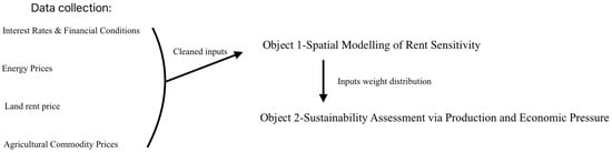
Figure 1.
Flowchart illustrating the 2-object analytical framework. (1) Spatial modelling of rent sensitivity based on geographically varying coefficient estimates. (2) Sustainability assessment through indicators of production and economic pressure, including yield volatility and the rent-to-revenue ratio (R2R).
2.1.1. Step 1: Spatial Modelling of Farmland Rents
Farmland rental prices are modelled as a function of macroeconomic indicators and agricultural variables. A geographically weighted regression (GWR) model is applied to capture spatial variation in parameter estimates and identify counties with high exposure to macroeconomic variability. As farm-level rental data are subject to confidentiality restrictions, the analysis is conducted at the county level. This step generates county-specific local coefficients that capture the sensitivity of rent to each macroeconomic factor.
2.1.2. Step 2: Sustainability Assessment of Agricultural Systems
To evaluate how macroeconomically driven rent dynamics affect agricultural sustainability by examining two key dimensions: production stability (measured by yield volatility) and economic pressure on farm operations (captured through the rent-to-revenue ratio). This objective identifies counties where high rental costs combined with unstable production conditions heighten vulnerability to economic shocks.
2.2. Study Field
The study area is defined to represent the core U.S. Corn Belt using an established geospatial framework based on maize production intensity. In this framework, the Corn Belt is characterised as a predominantly contiguous region with sustained and intensive maize cultivation, quantified using the modified areal fraction of corn () derived from satellite-based Crop Data Layer products. Counties with values exceeding 0.2 are identified as belonging to the core Corn Belt. This threshold has been widely adopted in previous studies to balance the inclusion of core maize-producing counties while avoiding peripheral or intermittent cultivation areas [18]. is calculated as follows:
where denotes the area classified as maize within a county, is the total county area, and is used to adjust for classification uncertainty and represents the user accuracy of maize classification. To account for the predominance of corn–soybean rotation systems, the methodology adopts a temporal averaging approach. By compiling data over an 18-year period (2007–2025), the analysis captures multiple crop rotation cycles. This multi-year averaging smooths short-term fluctuations arising from annual crop switching at the field level, thereby providing a stable and quantifiable representation of long-term maize cropping intensity rather than a single-year snapshot. Figure 2a illustrates the Corn Belt states considered in this study, consistent with commonly recognised regional definitions in the literature. Figure 2b presents the resulting county-level core Corn Belt delineation obtained using the based criterion. The selected counties form a largely contiguous spatial region without artificial gaps aligning closely with established representations of the core Corn Belt.
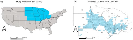
Figure 2.
Study area and delineation of the core U.S. Corn Belt. (a) Corn Belt states included in this study (blue). (b) County-level core Corn Belt delineated using the modified areal fraction of corn criterion (), following an established geospatial framework based on maize production intensity (light blue). The selected counties form a largely contiguous region consistent with commonly recognised representations of the core Corn Belt. The arrow indicates north, and uppercase labels denote U.S. state abbreviations.
2.3. Data Sources
This study integrates agricultural and macroeconomic datasets to examine the spatial sensitivity of farmland rental prices and their sustainability implications across the core Corn Belt. All datasets used in this analysis are publicly available, ensuring transparency and reproducibility (Table 1).

Table 1.
Input selection.
County-level cropland cash rents are obtained from the U.S. Department of Agriculture (USDA) National Agricultural Statistics Service (NASS) (Washington, DC, USA), which provides consistent annual estimates widely used in farmland market studies. County-level maize yield data are also sourced from the USDA and used both as a key explanatory variable and to identify the study sample. State-level maize prices from the USDA NASS are used to compute the rent-to-revenue ratio (R2R), an indicator of economic pressure on farm systems.
Macroeconomic information is collected from publicly accessible U.S. federal databases. Annual West Texas Intermediate (WTI) crude oil prices are obtained from the U.S. Energy Information Administration (EIA) (Washington, DC, USA), while the 10-year Treasury constant-maturity yield (St. Louis, MO, USA) and Gross Domestic Product Growth Rate are retrieved from the Bureau of Economic Analysis (Washington, DC, USA). National-level macroeconomic indicators are assumed to represent common external economic conditions faced by all counties, while spatial heterogeneity is captured through locally varying rent responses in the GWR framework. These indicators capture energy market conditions, capital costs, and aggregate economic activity that may influence rental market.
2.4. Data Integration and Preprocessing
In this study, all observations are aggregated to the county level using geographic coordinates. Temporal coverage is then assessed by counting the number of available years for each county. Counties with observations from only a single year are assigned entirely to the training set to maximise data utilisation.
For counties with multi-year records, at least one year is randomly selected to form the test set, while the remaining years are allocated to the training set. This splitting strategy accounts for uneven temporal coverage across counties. Because not all counties report data for every year, using a single common test year would exclude locations with incomplete records and reduce spatial representativeness. Randomly withholding one year per county when multi-year observations are available preserves separation while maximising data utilisation and maintaining broad geographic coverage. A total of 5262 samples are available for analysis, of which 4210 are used for training and 1052 for testing. This procedure helps reduced dependence between training and testing samples and increases the likelihood that counties with richer temporal coverage are represented in the test set, thereby improving regional representativeness.
2.5. Methodology
The methodological design follows the three research objectives outlined in the Introduction and integrates spatial econometrics, economic indicators, and sustainability risk assessment within a unified analytical structure.
2.5.1. Lagged Correlation Analysis Framework
Lagged correlation analysis allows for researchers to examine whether changes in one variable are temporally associated with subsequent movements in another variable, rather than occurring contemporaneously [19]. In the context of this study, this approach is applied to evaluate whether earlier fluctuations in agricultural, financial, or macroeconomic indicators contribute to subsequent movements in farmland rental prices. For each input feature , its correlation with farmland rent at different lag periods is calculated:
where represents the Pearson correlation coefficient at lag . By shifting feature values backward by years within each state and county, this method captures the temporal dependencies between historical changes in yield, commodity prices, interest rates, and macroeconomic factors with current farmland rent. Identifying significant lagged relationships provides insights into long-term trends. The larger the absolute value of indicates stronger temporal associations at the corresponding lag.
2.5.2. Multicollinearity Diagnosis and Variable Screening
The variance inflation factor (VIF) is employed in this study as a diagnostic tool to assess the extent of multicollinearity among the candidate explanatory variables [20]. Multicollinearity arises when predictors exhibit strong intercorrelations, which can inflate the variance of coefficient estimates and reduce model stability. When present, it becomes difficult to distinguish the individual contribution of each variable, thereby weakening the interpretability and overall reliability of the regression results [21].
where represents the coefficient of determination from regressing the variable on all remaining predictors. The resulting VIF value provides a diagnostic for the extent of multicollinearity. In general, a VIF of less than 5 is considered acceptable and indicates minimal collinearity concerns. Values between 5 and 10 signal a moderate level of multicollinearity. Importantly, in this study VIF is not used as an automatic variable elimination rule, but rather as a diagnostic indicator to identify potential redundancy and guide subsequent structural evaluation of explanatory variables.
When multicollinearity is detected, isolating the independent contribution of individual variables becomes challenging, particularly in systems where economic and commodity indicators are intrinsically interconnected. Bayesian network approaches could explicitly model joint distributions and dependency structures [22,23]; nevertheless, this approach requires large, regionally disaggregated samples to achieve stable inference, a condition not met in the present dataset.
2.5.3. Object 1—Spatial Modelling of Rent Sensitivity
Before applying the geographically weighted regression (GWR) model, a global spatial autocorrelation analysis is conducted to examine whether farmland rental prices exhibit statistically significant spatial dependence across counties. Identifying spatial autocorrelation provides a useful diagnostic for assessing whether spatial processes may vary across locations and whether global modelling assumptions may be violated.
Global Moran’s I is employed to quantify the overall degree of spatial autocorrelation in county-level farmland rental prices. The statistic is defined as
where is the number of spatial units (counties), and denote farmland rent values at locations and , is the global mean of farmland rent, and represents the spatial weight between counties and . is the sum of all spatial weights.
Moran’s I typically ranges between −1 and 1, where positive values indicate spatial clustering, negative values reflect spatial dispersion, and values near zero suggest the absence of global spatial structure [24]. To determine whether the observed statistic departs meaningfully from spatial randomness, a permutation-based p-value is computed. In addition, a corresponding Z-score is reported to indicate the degree to which the observed Moran’s I deviates from its expected value under the null hypothesis of spatial randomness. This p-value quantifies the probability of obtaining I value as extreme as the observed one under the null hypothesis of no spatial autocorrelation; small values (e.g., p < 0.05) provide evidence of significant spatial dependence, whereas large values imply that the spatial distribution is statistically indistinguishable from randomness.
To identify the local spatial structure of farmland rental prices, Local Indicators of Spatial Association (LISA) is further employed. LISA decomposes global spatial autocorrelation into location-specific statistics, allowing for the detection of local clusters and spatial outliers [25].
In this study, Local Moran’s I is calculated for each county to identify statistically significant High–High, Low–Low, High–Low, and Low–High spatial associations in farmland rental prices. High–High and Low–Low clusters indicate areas where counties with similar rent levels are surrounded by neighbours with comparable values, whereas High–Low and Low–High patterns represent spatial outliers. Statistical significance is assessed using a permutation-based approach.
Geographically weighted regression (GWR) is a spatial modelling technique that enables regression coefficients to vary across locations, allowing for relationships between the dependent and explanatory variables to change over space. In contrast to global regression models—which assume that a single set of parameters applies uniformly across the entire study area—GWR captures spatial heterogeneity by estimating location-specific coefficients [26]. The method employs a spatial weighting kernel in which observations closer to the focal location receive greater weight, while more distant observations contribute less, thereby producing a locally calibrated model.
This framework is particularly suited for analysing farmland rental prices, where localised conditions such as market accessibility, transportation networks, infrastructure, and regional economic activity can create substantial spatial variation [27]. Conventional regression approaches may overlook these geographically distinct influences, potentially leading to biased or overly generalised estimates. GWR mitigates this issue by fitting separate local regressions at each county, allowing for the influence of macroeconomic and agricultural variables on rent to differ across regions. This provides a more refined understanding of spatial market dynamics and enhances the interpretability of rental price determinants for land use planning and policy analysis. The general specification of GWR is expressed as follows [28]:
In a geographically weighted regression (GWR) framework, the coefficient for each predictor is estimated at the specific spatial coordinates , enabling the relationship between variables to vary across locations. The local intercept reflects the expected value of the dependent variable at that location when all predictors are held constant. The disturbance term is assumed to be normally distributed with constant variance, representing unexplained local variation in the model.
The spatial weighting matrix represents the degree of influence that observation j has on the estimation of local parameters at location i. This matrix governs how information from nearby locations is incorporated into the calibration of each coefficient , assigning greater weight to observations that are spatially closer and diminishing the influence of those farther away.
Weights are determined by a kernel function that quantifies spatial proximity between pairs of observations. One of the most applied kernels in GWR is the Gaussian function, which specifies the weight between locations i and j as follows [28]:
The spatial distance between observations, denoted as , is a key determinant of how much influence location exerts on the parameter estimates at location within the GWR framework. The degree of this influence is governed by the bandwidth parameter , which defines the scale over which neighbouring observations contribute to the local regression. A smaller bandwidth assigns greater importance to nearby points and underlines fine-grained spatial patterns, whereas a larger bandwidth incorporates information from a broader area, producing estimates that resemble a more global model.
Selecting an appropriate bandwidth is essential for balancing local detail with regional stability. In this study, the optimal bandwidth is determined by minimising the corrected Akaike Information Criterion (), a standard approach widely used for GWR model calibration [29]:
where L is the maximum likelihood of the model. represents the number of estimated parameters, including the intercept and all local regression coefficients. is the total number of observations used in the model. The first component, , reflects the goodness of fit, with smaller values indicating better agreement between the model and the observed data. The term penalises model complexity by increasing the score as more parameters are added, thereby discouraging overfitting. The final adjustment term, , further penalises models when the number of parameters approaches the sample size, ensuring more reliable inference in settings where local estimation reduces the effective degrees of freedom. The bandwidth in the GWR model is selected by minimising the corrected Akaike Information Criterion (AICc). AICc is adopted because it explicitly balances model goodness-of-fit and model complexity, making it well suited to geographically weighted regression where increased flexibility may otherwise lead to overfitting. Compared with alternative criteria such as cross-validation, AICc provides a theoretically grounded and widely used approach for bandwidth optimisation in spatially structured datasets with multiple explanatory variables [30].
Assessing uncertainty is a crucial component of geographically weighted regression (GWR), as it provides information on the robustness of the locally estimated coefficients. A commonly used measure of such uncertainty is the standard error (SE), which reflects the degree of variability in the parameter estimates across space [31]. Examining Ses allows for researchers to distinguish meaningful spatial patterns in coefficient estimates from variation that may simply arise due to sampling noise.
The computation of local standard errors relies on the GWR hat matrix , which represents the influence that each observation exerts on the local parameter estimates [32]. The standard error of a coefficient at location i is given by
where is the estimated variance of the residuals; is the diagonal element of the hat matrix, representing the leverage of observation i.
For the sensitivity analysis of mean farmland rent predictions, the local coefficients generated by the geographically weighted regression (GWR) model are utilised. Because GWR is a linear modelling framework, each coefficient directly reflects the marginal contribution of its corresponding variable to rental price variation. Examining these coefficients across geographic locations reveals how the influence of each factor changes spatially.
2.5.4. Object 2—Sustainability Assessment via Production and Economic Pressure
To evaluate how farmland rent dynamics influence agricultural sustainability, this study focuses on two key dimensions: production stability and economic pressure. Production stability is measured through yield volatility, which quantifies the temporal variability in maize yields. Yield volatility is computed using the standard deviation of year-on-year log differences:
denotes the maize yield in county at time , and is the number of years considered. Higher volatility indicates reduced production stability and greater exposure to biophysical and market uncertainties. A higher yield volatility value indicates greater interannual variability in maize production, reflecting lower production stability and higher exposure to climatic or market shocks.
Economic pressure is captured using the rent-to-revenue ratio, which measures the share of gross crop revenue required to cover land rental expenses [33]:
This ratio reflects how sensitive farm profitability is to rental costs. Larger values imply tighter margins and a diminished capacity for farmers to absorb economic shocks or adopt sustainable practices. For example, if a county pays USD 250/acre in rent but generates only USD 600/acre in crop revenue, its R2R will be much higher than a county with the same rent but USD 900/acre in revenue, indicating greater financial pressure.
2.5.5. Evaluation Criteria
The coefficient of determination (COD) is widely used to assess the accuracy and explanatory power of predictive models by measuring how well the predicted outcomes align with the observed data [34]. It represents the fraction of total variation in the dependent variable that can be attributed to the model rather than random noise, thereby indicating how effectively the model captures key relationships in the dataset [35]. The formula for COD is as follows:
where is the mean values. is the predicted value. A COD value approaching 1 indicates that the model accounts for most of the variability in the observed data, reflecting strong predictive capability. Conversely, values near zero imply that the model performs poorly and fails to explain the underlying variation in the target variable.
The importance of each explanatory variable is evaluated by examining the variability of its local regression coefficients, quantified through their standard deviation across all geographic locations [36]. The coefficient variability can be calculated:
A larger value of indicates stronger spatial heterogeneity, meaning the effect of that variable differs substantially from one county to another. Conversely, a smaller value suggests that the variable’s impact is relatively stable throughout the study area.
The confidence interval (CI) is used to quantify prediction uncertainty. To avoid data leakage, standard errors applied to the test set are estimated from the training set rather than recalculated on test observations. Using training-derived variance preserves out-of-sample independence and ensures an unbiased assessment of predictive uncertainty. The CI in this study is defined as follows [37]:
The quality of the confidence interval can be evaluated using the coverage rate, which measures the proportion of predictions falling within the 95% CI. A well-calibrated interval should capture close to 95% of the samples, with an acceptable range of roughly 92–97% due to natural model and data variability.
3. Results
3.1. Result of Lagged Correlation Analysis
The lagged correlation between farmland rent and key input variables, including yield, maize price, oil price, the Dollar Index, the 10-year Treasury yield, PCE, and GDP growth rate are summarised in Table 2. The results show that yield reaches its strongest positive correlation with rent at a 1-year lag, suggesting that rental markets may respond gradually to changes in agricultural productivity. In contrast, PCE and GDP growth rate display their highest positive correlations at a one-year lag. The 10-year Treasury yield shows its strongest negative correlation with rent at a 1-year lag, indicating that rising long-term interest rates increase financing costs and suppress rental price growth.
Table 2.
Lagged correlation for 5 years.
Although different variables affect rent over distinct lag periods, this study employs a one-year lag in the modelling process, as six of the key inputs display their strongest relationship at this interval. Using a one-year lag provides a practical balance between short-term responses and longer-term adjustments while capturing the dominant drivers of rental dynamics.
Multicollinearity is examined using variance inflation factors (VIFs). As shown in Table 3, all variables present VIF values within an acceptable range, suggesting that multicollinearity is not a major concern for the selected model inputs.
Table 3.
Variance inflation factors (VIFs) for original inputs.
Despite the absence of strong statistical multicollinearity, further inspection from an economic interpretation perspective reveals that personal consumption expenditure (PCE) represents a core component of aggregate economic activity and conveys information that largely overlaps with GDP growth rate. Although PCE is retained in the initial analysis to capture consumption-related macroeconomic effects, its inclusion alongside GDP growth rate offers limited additional explanatory value. To improve model parsimony and interpretability, and to avoid redundancy in representing similar macroeconomic dynamics, PCE is therefore excluded from subsequent analyses, whereas GDP growth is retained as a broader indicator of macroeconomic conditions.
Global Moran’s I is applied to examine the presence of spatial dependence in farmland rental prices in Table 4. The Moran’s I value is 0.6512, accompanied by a highly significant p-value (p = 0.001), indicating strong positive spatial autocorrelation across the study area. The corresponding Z-score further confirms that the observed spatial clustering of rental prices departs substantially from spatial randomness. The large Z-score reflects the substantial sample size and strong spatial clustering rather than an anomalous test statistic.
Table 4.
Global Moran’s I for rent cost.
Consistent with the global statistic, the LISA cluster map (Figure 3) reveals pronounced High–High clusters concentrated in the central Corn Belt, while Low–Low clusters are primarily located in peripheral regions. These results demonstrate clear spatial dependence in farmland rental prices, providing empirical support for the application of local spatial modelling approaches.
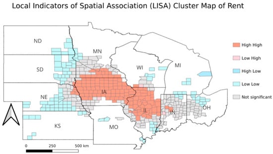
Figure 3.
Local Indicators of Spatial Association (LISA) cluster map of county-level farmland rental prices in the core Corn Belt.
3.2. Results of Object 1—Spatial Modelling of Rent Sensitivity
Although strong global spatial dependence is observed in farmland rents, this does not imply spatial stationarity in the relationships between farmland rent and its determinants. To examine whether the sensitivities of macroeconomic and agricultural variables vary across space, a geographically weighted regression (GWR) framework is adopted to capture spatial heterogeneity in model parameters.
The ordinary least squares (OLS) results (Figure 4a) show limited predictive capability, as the model does not adequately capture key relationships in the data. Moreover, the test COD (0.38) slightly exceeds the training COD (0.33), reflecting limited explanatory power and suggesting that the global model fails to adequately capture the underlying structure of farmland rent variation. In contrast, the GWR model (Figure 4b) achieves substantially better performance, with both training and test COD values reaching 0.87. The close alignment between the two sets demonstrates strong generalisability and indicates that GWR effectively accounts for spatial differences in variable influence.
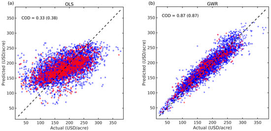
Figure 4.
Performance of linear regression and GWR model ((a) result of linear regression; (b) result of GWR model). The dashed line represents the 1:1 line indicating perfect agreement between predicted and observed values. Blue and red dots denote training and testing samples, respectively.
Beyond predictive accuracy, model performance is further evaluated using the corrected Akaike Information Criterion (AICc) in Table 5, which explicitly accounts for differences in model complexity. As reported in Table 5, the GWR model yields a substantially lower AICc value (38,767) than the OLS model (44,059). This result confirms that the improved fit of the GWR model is not solely driven by over-parameterisation but reflects its enhanced ability to capture spatial non-stationarity in the relationships between farmland rent and its determinants.
Table 5.
AICc for GWR and OLS model.
For the uncertainty-enhanced GWR model, the results are presented in Figure 5. The negative log-likelihood (NLL) remains stable at 4.43 across datasets, indicating reliable likelihood estimation. Furthermore, the 95% confidence interval captures 96% of the test samples, suggesting that the uncertainty estimates are well calibrated and appropriately represent prediction variability.
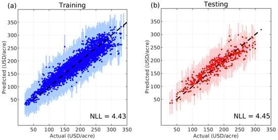
Figure 5.
Uncertainty performance of GWR models (vertical lines represent 95% credible interval; (a) result of GWR training set; (b) result of GWR testing set).
The probability density distribution of standard errors (Ses) for both the training and test sets is presented in Figure 6. Although the histograms may visually appear relatively uniform due to bin width and the narrow range of SE values, the underlying distributions are not uniform. Instead, both sets exhibit a unimodal pattern centred around approximately 21, with SE values ranging from about 18 to 25. This narrow spread is expected because the GWR model applies a consistent bandwidth across locations, resulting in locally weighted regressions with similar leverage structures.
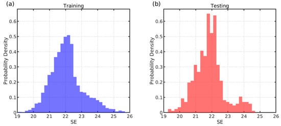
Figure 6.
Probability density distribution of standard errors (Ses) ((a) probability density distribution of SE in training set; (b) probability density distribution of SE in testing set).
The close alignment between the two distributions indicates that the model maintains a stable and coherent uncertainty structure rather than exhibiting overfitting or excessive confidence. The similarity between training and testing SE patterns therefore reinforces the reliability of the uncertainty estimation.
The feature importance results in Table 6 show that Dollar Index exhibits the strongest spatial heterogeneity (9.13), indicating that currency fluctuations exert the most spatially heterogeneous effect on farmland rental prices. Maize Price (8.48) and the 10-year Treasury yield (6.65) also display substantial variability, suggesting that market expectations and financial conditions contribute meaningfully to regional differences in rent sensitivity. Oil Price (6.31) shows a moderate level of spatial variation, while Yield (5.53) and GDP Growth (5.43) exert comparatively more stable effects across counties.
Table 6.
Spatial variability of GWR coefficients.
Figure 7 shows that uncertainty appears relatively uniform at the interstate scale, but clear differences emerge at the county level. Counties within the same state display varying standard errors. Local conditions and market dynamics contribute to meaningful variation in prediction uncertainty.
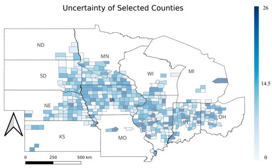
Figure 7.
County-level uncertainty quantification map.
The distribution of weight of each feature is presented as Figure 8. It illustrates how the influence of key variables on farmland rental prices varies across counties.
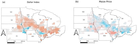
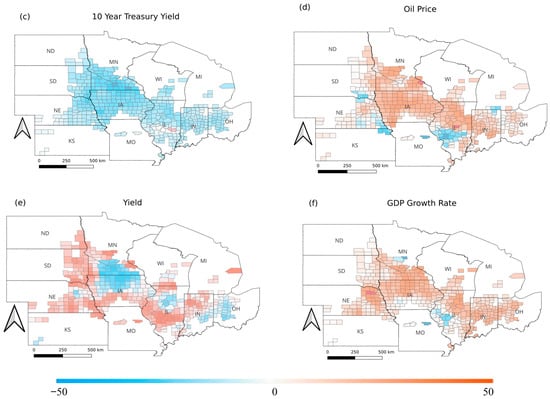
Figure 8.
County-level weight distribution of different features ((a) Dollar Index, (b) Maize Price, (c) 10-Year Treasury Yield, (d) Oil Price, (e) Maize Yield, (f) GDP Growth Rate).
The Dollar Index (Figure 8a) exhibits predominantly positive coefficients across the central Corn Belt, with stronger effects concentrated in Iowa, Illinois, and parts of Indiana, while weaker or negative effects appear in peripheral counties.
Maize price (Figure 8b) exhibits a mixed spatial pattern, with a localised positive band in the central part of the region and predominantly negative coefficients across the eastern counties.
The 10-year Treasury yield (Figure 8c) displays a largely consistent negative relationship with farmland rent across most counties, particularly in the central and western portions of the region, suggesting a broadly uniform sensitivity of rental markets to long-term interest rates. In contrast, oil price effects (Figure 8d) are spatially uneven, with stronger positive coefficients clustered in the central Corn Belt and weaker or mixed responses elsewhere.
Maize yield (Figure 8e) exhibits a mixed and locally clustered pattern, with negative coefficients forming noticeable clusters in the central Corn Belt (particularly across parts of Iowa) and extending into sections of Indiana and Ohio, while positive coefficients are more prevalent along western and southern margins. GDP growth rate (Figure 8f) is mostly positive across the region, but a clear negative cluster is observed around the Missouri–Illinois corridor.
3.3. Results of Object 2—Sustainability Assessment via Production and Economic Pressure
Building on the findings from Objective 1, which identified the spatially varying influence of economic and macroeconomic drivers on farmland rent, Objective 2 evaluates the sustainability implications of these rental dynamics. The spatial distribution of maize yield volatility across the core Corn Belt is illustrated as Figure 9a. The pattern does not display a clear regional structure. Within states such as Iowa, counties with low volatility sit alongside others with much higher volatility, indicating that stability in production varies strongly at the local scale. The yield volatility is shaped more by local conditions than by broad state-level differences. Figure 9b presents the spatial distribution of the rent-to-revenue ratio, which reflects the long-term economic pressure faced by farmers across the core Corn Belt. The map shows a clear spatial trend, with higher values concentrated in the central area of the region and gradually lower values toward the east. Higher ratios are mainly found in Illinois, Indiana, and parts of Ohio, showing that farmers in these areas must allocate a larger share of crop revenue to pay for land rent. This pattern suggests tighter profit margins and stronger financial pressure on producers in these counties.
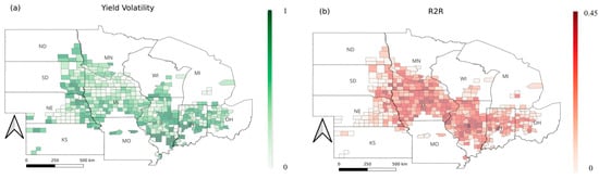
Figure 9.
Spatial patterns of (a) yield volatility and (b) the rent-to-revenue ratio (R2R) across the core Corn Belt counties. Different colour scales are used for each panel to reflect the distinct units and ranges of the two indicators; colour intensities should therefore be interpreted within, rather than across, panels.
4. Discussion and Limitation
4.1. Addressing the Research Gaps
This study responds directly to several limitations noted in the existing literature by integrating spatial modelling with an explicit assessment of predictive uncertainty. First, the incorporation of standard errors, confidence intervals, and coverage rates provides a transparent evaluation of model robustness, addressing the common absence of uncertainty quantification in farmland rent studies. This step is essential because macroeconomic conditions may interact in distinct ways with local production systems, which means that regional results cannot be fully interpreted without an understanding of estimation variability. Second, this study moves beyond conventional analyses that view rental prices solely as an economic outcome. Instead, it examines how rental dynamics can mediate the influence of macroeconomic signals on the long-term sustainability of agricultural regions. Third, the proposed framework combines macroeconomic exposure, economic pressure, and biophysical resilience to identify areas that may be more vulnerable under uncertain future conditions.
4.2. Interpretation of Spatial Patterns
The absence of a clear regional structure in both prediction uncertainty and yield variability suggests that sustainability-related risks in the core Corn Belt are governed primarily by local-scale processes rather than broad geographic gradients. This suggests that production stability and predictive uncertainty depend primarily on local agronomic conditions, management practices, or farm-specific characteristics rather than broader regional structures [38]. The absence of a regional trend also indicates that geographic position alone does not shape these aspects of sustainability risk, which supports findings that production variability is often driven by micro-scale climate differences, soil water conditions, and field management strategies.
Interestingly, some metropolitan counties do not emerge as major sources of noise despite their complex land use and limited agricultural production. This may be due to the county-level aggregation of variables, which captures broader economic conditions rather than parcel-level heterogeneity. Once aggregated, the influence of urban centres becomes moderated, allowing for the model to retain stability even in mixed land use environments.
4.3. Comparison with Existing Literature
The observed localised pattern of yield variability aligns with previous work suggesting that production risk is heavily influenced by microclimate variability, water availability, and farm-level management decisions. These findings are consistent with studies that identify within-county heterogeneity as a major determinant of yield stability, often exceeding differences observed between states [39]. The role of oil prices and interest rates in shaping rental patterns is also in line with research linking agricultural markets to broader macroeconomic conditions, particularly through the energy and financial sectors [40]. However, the present study extends the literature by demonstrating that macroeconomic exposure interacts with local production conditions to influence sustainability risk, a relationship that remains underexplored in most empirical analyses of farmland rents.
4.4. Policy Implications
The findings of this study also provide implications for understanding how the Renewable Fuel Standard shapes farmland rent dynamics and long-term sustainability in the core Corn Belt. Counties that show high rental pressure, greater yield variability, and strong responsiveness to macroeconomic signals may be more sensitive to policy-induced changes in maize demand. In such regions, expansions in ethanol production can amplify existing pressures by increasing competition for land and reinforcing the connection between energy markets and agricultural production [41]. Policy adjustments that stabilise biofuel demand or reduce volatility in the ethanol market could therefore help moderate rental pressures and support more sustainable land use decisions.
In areas where macroeconomic exposure is strong, changes in energy prices or financial conditions may interact with the RFS in ways that heighten production risk [41]. Supporting credit access, improving risk management programs or enhancing the flexibility of compliance mechanisms could reduce the vulnerability of these regions to policy-driven shocks. In addition, the lack of a consistent spatial pattern in uncertainty and yield variability suggests that RFS-related impacts will not be uniform. Local governance and county-level advisory programs remain particularly important, since the consequences of the RFS are likely to vary across short distances and cannot be inferred from state-level averages.
4.5. Limitations
4.5.1. Model Complexity and Local Degrees of Freedom
Although the GWR model achieves a high coefficient of determination, locally varying coefficients increase the effective degrees of freedom and may introduce a risk of overfitting. To mitigate this concern, model performance is evaluated in conjunction with information-based criteria, particularly the corrected Akaike Information Criterion (AICc), which explicitly penalises model complexity. Nevertheless, COD values should be interpreted with caution and not in isolation.
The county-level aggregation adopted in this study smooths short-term variability associated with field-level management and crop rotation. While this aggregation is appropriate for capturing long-term structural relationships between economic drivers and farmland rents, it may obscure finer-scale heterogeneity. Finally, the analysis focuses on realised economic and production outcomes and does not explicitly model all underlying biophysical drivers, which represents a trade-off between interpretability and model scope.
Whilst the proposed spatial modelling framework remains broadly applicable, the empirical results primarily reflect dynamics inherent to the core Corn Belt; consequently, they may not directly generalise to regions characterised by lower production intensity, disparate cropping systems, or alternative land market structures.
4.5.2. Data Aggregation and Omitted Variables
Although the temporal train–test split is employed to reduce information leakage across time, complete independence between training and testing samples cannot be fully guaranteed in the presence of strong spatial autocorrelation. Farmland rental prices and their covariates exhibit persistent spatial structures across neighbouring counties, which may lead to similar predictive performance across temporally separated samples. This characteristic reflects an inherent property of spatial economic systems rather than model overfitting.
In addition, because the analysis is conducted at the county scale, year-to-year crop rotation effects are largely smoothed yet not fully removed. The absence of finer-scale rental data stems from the private nature of farmland rental contracts, which cannot be accessed in public databases, making county-level aggregation the most feasible resolution. In addition, the exclusion of explicit biophysical variables such as soil quality and microclimate may introduce omitted variable bias if these factors are correlated with both farmland rents and economic drivers. Although many biophysical characteristics are relatively stable over time and partially reflected in the spatial structure captured by GWR, their omission may lead to an upward bias in the estimated sensitivities of economic variables in regions where favourable natural conditions coincide with stronger market signals.
4.6. Future Directions
Future research may extend the present framework by incorporating Bayesian and simulation-based approaches to provide a more comprehensive characterisation of spatial uncertainty. Bayesian geographically weighted regression (BGWR) could be employed to estimate full posterior distributions of location-specific coefficients, allowing for uncertainty to be explicitly propagated across space and facilitating probabilistic inference on regional rent sensitivities. In addition, Monte Carlo simulation techniques could be integrated to assess the robustness of estimated coefficients under alternative sampling schemes, bandwidth choices, and stochastic perturbations in explanatory variables. Such extensions would enable a richer assessment of uncertainty and risk in farmland rental markets, especially under scenarios of heightened macroeconomic volatility, while complementing the deterministic GWR framework adopted in this study.
5. Conclusions
This study examined the spatial and economic determinants of farmland rental prices in the core Corn Belt by integrating spatial modelling with an explicit assessment of predictive uncertainty. By linking macroeconomic exposure, rental market pressure, and production stability, the analysis offers a comprehensive perspective on the sustainability of agricultural systems. Using geographically weighted regression, the analysis revealed substantial spatial variation in the sensitivity of rental prices to macroeconomic factors such as oil prices, interest rates, and economic activity. These findings highlight that rental markets serve as an important channel through which broader economic conditions influence land use decisions and long-term resilience.
Despite pronounced spatial variation in rental sensitivities, neither prediction uncertainty nor maize yield volatility exhibits a coherent regional structure. Instead, both remain highly localised, highlighting that agricultural vulnerability and model reliability are governed primarily by county-level conditions rather than broad geographic patterns. This finding emphasises the necessity of localised analysis when evaluating sustainability risks in intensive agricultural regions.
Methodologically, this study contributes an uncertainty-aware, spatially explicit perspective on farmland rent dynamics that extends beyond conventional global modelling approaches. By jointly examining spatially varying rent sensitivities, production instability, and economic pressure, the framework enables a more nuanced understanding of how macroeconomic shocks interact with local production conditions to influence sustainability outcomes.
From a policy perspective, the findings suggest that regions characterised by high rental pressure and strong macroeconomic exposure may be particularly sensitive to fluctuations in energy and financial markets, including those associated with biofuel policies such as the Renewable Fuel Standard. These results support the need for place-based agricultural policies and region-specific risk management strategies rather than uniform interventions.
While the analysis is subject to limitations related to county-level aggregation and the omission of some biophysical drivers, the proposed framework offers a scalable foundation for future research incorporating finer-scale data and probabilistic modelling approaches to further assess spatial uncertainty and policy impacts under evolving economic conditions.
Author Contributions
Conceptualization, S.L. and X.H.; methodology, S.L. and X.H.; software, S.L.; validation, S.L. and X.H.; formal analysis, S.L.; investigation, S.L.; resources, S.L.; data curation, S.L.; writing—original draft preparation, S.L.; writing—review and editing, X.H.; visualization, S.L. and X.H.; supervision, X.H.; project administration, X.H. All authors have read and agreed to the published version of the manuscript.
Funding
This research received no external funding.
Institutional Review Board Statement
Not applicable.
Informed Consent Statement
Not applicable.
Data Availability Statement
The data presented in this study are available on request.
Conflicts of Interest
The authors declare no conflicts of interest.
Abbreviations
| AICc | Akaike Information Criterion |
| AWC | Available Water Capacity |
| BEA | Bureau of Economic Analysis |
| COD | Coefficient of Determination |
| CME | Chicago Mercantile Exchange |
| CI | Credible Interval |
| DXY | USA Dollar Index |
| EIA | Energy Information Administration |
| GDP | Gross Domestic Product |
| GWR | Geographically Weighted Regression |
| OLS | Ordinary Least Squares |
| PCE | Personal Consumption Expenditure |
| SE | Standard Error |
| USDA | United States Department of Agriculture |
| VIF | Variance Inflation Factor |
| WTI | West Texas Intermediate |
References
- Erenstein, O.; Jaleta, M.; Sonder, K.; Mottaleb, K.; Prasanna, B.M. Global maize production, consumption and trade: Trends and R&D implications. Food Secur. 2022, 14, 1295–1319. [Google Scholar] [CrossRef]
- Teste, F.; Makowski, D.; Bazzi, H.; Ciais, P. Early forecasting of corn yield and price variations using satellite vegetation products. Comput. Electron. Agric. 2024, 221, 108962. [Google Scholar] [CrossRef]
- Lee, U.; Kwon, H.; Wu, M.; Wang, M. Retrospective analysis of the U.S. corn ethanol industry for 2005–2019: Implications for greenhouse gas emission reductions. Biofuels Bioprod. Biorefining 2021, 15, 1318–1331. [Google Scholar] [CrossRef]
- Fuglie, K. R&D Capital, R&D Spillovers, and Productivity Growth in World Agriculture. Appl. Econ. Perspect. Policy 2017, 40, 421–444. [Google Scholar] [CrossRef]
- Li, S.; He, X. Quantifying Policy-Induced Cropland Dynamics: A Probabilistic and Spatial Analysis of RFS-Driven Expansion and Abandonment on Marginal Lands in the U.S. Corn Belt. Sustainability 2025, 17, 9568. [Google Scholar] [CrossRef]
- McPhail, L.L.; Babcock, B.A. Impact of US biofuel policy on US corn and gasoline price variability. Energy 2012, 37, 505–513. [Google Scholar] [CrossRef]
- Lark, T.J.; Spawn, S.A.; Bougie, M.; Gibbs, H.K. Cropland expansion in the United States produces marginal yields at high costs to wildlife. Nat Commun 2020, 11, 4295. [Google Scholar] [CrossRef]
- Baldos, U.L.C.; Hertel, T.W. The role of international trade in managing food security risks from climate change. Food Secur. 2015, 7, 275–290. [Google Scholar] [CrossRef]
- Gospodarowicz, M.; Karwat-Woźniak, B.; Ślązak, E.; Wasilewski, A.; Wasilewska, A. Agricultural Land Market Dynamics and Their Economic Implications for Sustainable Development in Poland. Sustainability 2025, 17, 6484. [Google Scholar] [CrossRef]
- Stevens, A.W.; Wu, K. Land tenure and profitability among young farmers and ranchers. Agric. Financ. Rev. 2021, 82, 486–504. [Google Scholar] [CrossRef]
- Stevens, A.W. The economics of land tenure and soil health. Soil Secur. 2022, 6, 100047. [Google Scholar] [CrossRef]
- Lin, S.-H.; Huang, X.; Fu, G.; Chen, J.-T.; Zhao, X.; Li, J.-H.; Tzeng, G.-H. Evaluating the sustainability of urban renewal projects based on a model of hybrid multiple-attribute decision-making. Land Use Policy 2021, 108, 105570. [Google Scholar] [CrossRef]
- Caraiani, P. The impact of oil supply news shocks on corporate investments and the structure of production network. Energy Econ. 2022, 110, 106011. [Google Scholar] [CrossRef]
- Gholipour, H.F.; Farzanegan, M.R.; Arjomandi, A.; Yam, S.; Gerth, F. Farmland prices and the farming industry’s profitability in Australia. Appl. Econ. 2025; online first. [Google Scholar] [CrossRef]
- Nag, S.; Reimer, J.J. Farmland cash rents and the dollar. Agric. Econ. 2011, 42, 509–517. [Google Scholar] [CrossRef]
- Keskin, G. Production costs and land appraisal: A case study of Polatlı, Turkey. Ciência Rural 2023, 53, e20210609. [Google Scholar] [CrossRef]
- Kvartiuk, V.; Bukin, E.; Herzfeld, T. “For whoever has will be given more”? Land rental decisions and technical efficiency in Ukraine. Land Use Policy 2024, 146, 107336. [Google Scholar] [CrossRef]
- Green, T.R.; Kipka, H.; David, O.; McMaster, G.S. Where is the USA Corn Belt, and how is it changing? Sci. Total Environ. 2018, 618, 1613–1618. [Google Scholar] [CrossRef]
- Wang, F.; Wang, L.; Chen, Y. Lagged multi-affine height correlation analysis for exploring lagged correlations in complex systems. Chaos 2018, 28, 061102. [Google Scholar] [CrossRef] [PubMed]
- Salmerón-Gómez, R.; García-García, C.B.; García-Pérez, J. A Redefined Variance Inflation Factor: Overcoming the Limitations of the Variance Inflation Factor. Comput. Econ. 2024, 65, 337–363. [Google Scholar] [CrossRef]
- Chalkias, C.; Polykretis, C.; Karymbalis, E.; Soldati, M.; Ghinoi, A.; Ferentinou, M. Exploring spatial non-stationarity in the relationships between landslide susceptibility and conditioning factors: A local modeling approach using geographically weighted regression. Bull. Eng. Geol. Environ. 2020, 79, 2799–2814. [Google Scholar] [CrossRef]
- Tiffin, R.; Balcombe, K. The determinants of technology adoption by UK farmers using Bayesian model averaging: The cases of organic production and computer usage. Aust. J. Agric. Resour. Econ. 2011, 55, 579–598. [Google Scholar] [CrossRef]
- Basnet, S.K.; Jansson, T.; Heckelei, T. A Bayesian econometrics and risk programming approach for analysing the impact of decoupled payments in the European Union*. Aust. J. Agric. Resour. Econ. 2021, 65, 729–759. [Google Scholar] [CrossRef]
- Shen, T.; Zhou, W.; Yuan, S.; Huo, L. Spatiotemporal Characterization of the Three-Dimensional Morphology of Urban Buildings Based on Moran’s I. Sustainability 2024, 16, 6540. [Google Scholar] [CrossRef]
- Lutz, S.U. The European digital single market strategy: Local indicators of spatial association 2011–2016. Telecommun. Policy 2019, 43, 393–410. [Google Scholar] [CrossRef]
- Neelawala, P.; Wilson, C.; Athukorala, W. The impact of mining and smelting activities on property values: A study of Mount Isa city, Queensland, Australia. Aust. J. Agric. Resour. Econ. 2012, 57, 60–78. [Google Scholar] [CrossRef]
- Paulson, N.D.; Schnitkey, G.D.; Sherrick, B.J. Rental arrangements and risk mitigation of crop insurance and marketing. Agric. Financ. Rev. 2010, 70, 399–413. [Google Scholar] [CrossRef]
- Fotheringham, A.S.; Charlton, M.E.; Brunsdon, C. Spatial Variations in School Performance: A Local Analysis Using Geographically Weighted Regression. Geogr. Environ. Model. 2001, 5, 43–66. [Google Scholar] [CrossRef]
- Akpa, O.M.; Unuabonah, E.I. Small-Sample Corrected Akaike Information Criterion: An appropriate statistical tool for ranking of adsorption isotherm models. Desalination 2011, 272, 20–26. [Google Scholar] [CrossRef]
- Almasi, S.A. Evaluating the efficiency of spatial-geographical models for vehicle crash frequency estimation: A case study on the urban road network of hamadan province. Transp. Eng. 2025, 21, 100362. [Google Scholar] [CrossRef]
- Ribeiro, M.C.; Pereira, M.J. Modelling local uncertainty in relations between birth weight and air quality within an urban area: Combining geographically weighted regression with geostatistical simulation. Environ. Sci Pollut. Res. Int. 2018, 25, 25942–25954. [Google Scholar] [CrossRef]
- Yu, H.; Fotheringham, A.S.; Li, Z.; Oshan, T.; Kang, W.; Wolf, L.J. Inference in Multiscale Geographically Weighted Regression. Geogr. Anal. 2019, 52, 87–106. [Google Scholar] [CrossRef]
- Jodlbauer, H.; Tripathi, S.; Bachmann, N.; Brunner, M.; Thienemann, A.-K.; Tüzün, A.; Pöchtrager, S. Cost and Profit Distributions in Allied Supply Chains. Procedia Comput. Sci. 2025, 253, 515–523. [Google Scholar] [CrossRef]
- Piepho, H.P. An adjusted coefficient of determination (R(2)) for generalized linear mixed models in one go. Biom. J. 2023, 65, e2200290. [Google Scholar] [CrossRef] [PubMed]
- Es-haghi, M.S.; Rezania, M.; Bagheri, M. Machine learning-based estimation of soil’s true air-entry value from GSD curves. Gondwana Res. 2023, 123, 280–292. [Google Scholar] [CrossRef]
- Acal, C.; Maldonado, D.; Aguilera, A.M.; Zhu, K.; Lanza, M.; Roldan, J.B. Holistic Variability Analysis in Resistive Switching Memories Using a Two-Dimensional Variability Coefficient. ACS Appl. Mater. Interfaces 2023, 15, 19102–19110. [Google Scholar] [CrossRef]
- Abdalla, O.; Walker, C.; Ishimori, K. R-code for calculating fluctuation assay results and 95% confidence intervals based on Ma–Sandri–Sarkar Maximum Likelihood. Softw. Impacts 2024, 21, 100661. [Google Scholar] [CrossRef]
- Salam, M.A. Exploring the seasonal yield variability, production risk and efficiency: The case of rice farms in Bangladesh. Heliyon 2022, 8, e10559. [Google Scholar] [CrossRef]
- Panda, S.S.; Siddique, A.; Terrill, T.H.; Mahapatra, A.K.; Morgan, E.; Pech-Cervantes, A.A.; van Wyk, J.A. Decision support system for Lespedeza cuneata production and quality evaluation: A WebGIS dashboard approach to precision agriculture. Front. Plant Sci. 2025, 16, 1520163. [Google Scholar] [CrossRef]
- Hisar, S.; Rosalina, S.S.; Rakhman, A.; Apriwenni, P.; Wolor, C.W. Navigating Inflation in Indonesia’s Agricultural Sector from 2016 to 2024: Insights into Profit Margins, Asset Turnover, and Earnings Per Share. Res. World Agric. Econ. 2025, 6, 67–81. [Google Scholar] [CrossRef]
- Lade, G.E.; Lin Lawell, C.Y.C.; Smith, A. Policy Shocks and Market-Based Regulations: Evidence from the Renewable Fuel Standard. Am. J. Agric. Econ. 2018, 100, 707–731. [Google Scholar] [CrossRef]
Disclaimer/Publisher’s Note: The statements, opinions and data contained in all publications are solely those of the individual author(s) and contributor(s) and not of MDPI and/or the editor(s). MDPI and/or the editor(s) disclaim responsibility for any injury to people or property resulting from any ideas, methods, instructions or products referred to in the content. |
© 2025 by the authors. Licensee MDPI, Basel, Switzerland. This article is an open access article distributed under the terms and conditions of the Creative Commons Attribution (CC BY) license.