Abstract
Technical change plays a crucial role in improving environmental quality, while the influence of demand-side factors remains insufficiently examined. To clarify the pull effect of consumer demand on the transition to clean technology, this study develops a model of directed technical change incorporating quality innovation in consumer goods. The analysis shows that the relative prices and market sizes of clean consumer goods drive the transition to clean technology, generating a direct demand-induced pull for clean innovations. Income inequality determines the market size of clean relative to dirty goods, thereby shaping innovation incentives and influencing the effectiveness of environmental policies. By integrating learning-by-doing and demand-induced innovation for dirty and clean technologies, respectively, the model captures the path dependence of technological progress and explains the dynamic ‘U-shaped’ evolution of environmental quality under environmental policy intervention. These findings provide theoretical insight into how consumer heterogeneity and income distribution affect the direction of innovation and the long-term transition toward cleaner technologies.
1. Introduction
1.1. Research Background
Technological change is pivotal in mitigating pollution emissions, reversing environmental degradation, and curbing climate change [1]. However, environmental externalities, knowledge spillovers, and technological path dependence collectively contribute to persistent market failures in environmental and climate-related sectors [2]. Consequently, the private sector faces insufficient incentives to foster clean innovation and improve energy efficiency. Accordingly, policy intervention aimed at redirecting technological progress is essential to facilitate the transition from dirty to clean technologies [3,4,5]. Recent research using a systems-based perspective finds that organizational and inter-firm network integration, together with managerial capabilities, critically shape the adoption of new technologies in enterprises [6]. For instance, Aghion et al. empirically examined firm-level innovation in the automotive industry and demonstrated that carbon taxation significantly stimulates clean innovations [7]. Acemoglu et al. further showed that carbon taxation and research and development (R&D) subsidies can incentivize innovation toward clean inputs, while delaying environmental policy implementation entails substantial welfare losses [8]. Without government intervention, clean innovation would eventually disappear, allowing dirty technologies to dominate the economy and leading to a projected temperature increase of approximately 11 degrees Celsius over two centuries [4].
Despite these contributions, the aforementioned studies require further improvements in the following aspects. (i) Existing analyses primarily focus on supply-side policy effects, neglecting the interconnections with consumer behavior and, consequently, the demand-pull channel through which consumer preferences influence clean innovation and environmental quality. In such frameworks, perfectly competitive final-good producers interact directly with consumers and, as a result, are unable to transmit the price adjustments induced by environmental policies. (ii) Under the standard assumption of homothetic preferences, consumption depends solely on income levels and is invariant to income distribution, which prevents the model from explaining the relationship between income inequality and consumption composition [9]. As emphasized by Acemoglu et al., incentives for clean innovation originate from production inputs—particularly the price effect of clean inputs and the market-size effect of labor—rather than from final consumption goods [4,8]. Therefore, these models provide an incomplete account of demand-induced innovation. (iii) These frameworks fail to capture the path dependence of dirty technologies under environmental policy regimes, and thus cannot reproduce the empirically observed “U-shaped” trajectory of environmental quality, which is often referred to as the Porter effect. When dirty and clean technologies compete in a symmetric setting of technological changes, all R&D resources in the economy are allocated entirely to dirty technology in the laissez-faire equilibrium. Under policy intervention, by contrast, all R&D resources are directed to clean technologies. Because dirty innovation ceases once environmental policies are enacted, these models cannot fully characterize the technological path dependence inherent in dirty sectors [4,8,10]. Furthermore, the complete reallocation of R&D resources induced by environmental policy—i.e., a corner solution—renders it difficult to rationalize the observed ‘U-shaped’ evolution of environmental quality [8], unless tax or subsidy rates are unrealistically high or the technological gap between clean and dirty sectors is excessively large [4].
1.2. Literature Background
This study is situated within three major strands of the existing literature.
The first strand examines the nexus between income inequality and environmental quality. The mainstream literature identifies three primary mechanisms. The first is the declining marginal propensity to emit based on consumption behavior [11,12,13]. The second focuses on the political-economy determination of environmental policy, emphasizing how income distribution shapes collective decision-making and regulatory stringency [14,15,16,17,18]. The third highlights the role of income inequality in influencing the innovation and diffusion of clean technologies [19,20].
In contrast to these perspectives, this study underscores the role of demand-induced clean innovation in enhancing environmental quality, with particular emphasis on the price and market-size effects arising from income inequality [9]. The main contribution of this paper lies in developing a general equilibrium model of consumer-goods quality upgrading to examine how income inequality shapes environmental outcomes. In our framework, income inequality serves as a pivotal driver of clean innovation, directly influencing both the direction of technological transition and environmental quality. This demand-oriented perspective complements recent systems-based research, which emphasizes that cross-sectoral coordination and industrial symbiosis can enhance technological innovation and sustainability by integrating environmental and technological project management [21].
The second strand relates to the theory of directed technical change in environmental economics. Our model demonstrates how the composition of consumers generates a demand-side pull that influences both the shift toward clean technology and improvements in environmental quality. Early contributions to endogenous technological change incorporated pollution-enhancing technologies [22], environmental constraints [23], and learning-by-doing effects [24]. However, these studies typically focus on a single type of innovation and do not explicitly capture the transition from dirty to clean technologies driven by environmental policy [25].
Acemoglu et al. developed two-sector endogenous growth models directed to clean-technology [4,8]. In their framework, the transition to clean technology is governed by relative input prices and the market size of production factors, with primary emphasis on supply-side mechanisms. Related research further shows that network integration among firms—such as cross-industry industrial symbiosis—can facilitate the development and diffusion of innovative technologies, thereby improving resource efficiency and environmental performance [21]. While this study shares the view of Acemoglu et al. hat directed technical change is a deliberate and profit-driven process, it departs from the existing literature in two important respects [4,8]. First, innovation incentives in our model arise from the relative trade-off between the price and market size of consumer goods, rather than from intermediate inputs or production factors. Second, unlike the supply-side focus emphasized by Acemoglu et al., our framework highlights a demand-pull mechanism, offering a complementary perspective on directed technical change in environmental economics [4,8].
The third strand of literature most closely related to this study concerns the relationship between income inequality and the effectiveness of environmental policy. From the perspective of policy formation, Boyce and Torras and Boyce show that rising income inequality may lead to environmental degradation [14,15], while income redistribution alters social demand for environmental quality [16], thereby generating “induced policy responses” to inequality [26,27]. A common hypothesis in this literature is that higher levels of economic inequality contribute to greater environmental degradation or less stringent environmental policies [28].
From the standpoint of policy effectiveness, environmental regulation must be designed and implemented in ways that accurately reflect individual preferences in order to encourage consumers and firms to internalize environmental externalities [29,30]. Because green technologies and green consumption goods are constrained by income levels and willingness to pay, income distribution plays a critical role in shaping the effectiveness of environmental policies [31]. For example, carbon pricing and green innovation subsidies are widely recognized as effective instruments for addressing global climate change; however, their design and policy outcomes could be further improved by explicitly accounting for income inequality [32]. For instance, Lebedev et al. developed humic acid-modified environmentally safe biodegradable films with antibacterial properties and high biodegradability, a typical case of demand-driven clean technology innovation in consumer goods [33]. In addition, Aghion et al. show that stronger environmental preferences can raise public environmental awareness, alleviate competitive pressure on firms, and stimulate greater investment in green technologies, yet they do not examine how income inequality conditions the effectiveness of environmental policy [34].
Overall, the classic theory of clean-technology bias largely neglects the direct demand-side pull on green innovation and fails to uncover the intrinsic link between income heterogeneity and optimal environmental policy design [8,35,36].
1.3. Research Objectives
To overcome these limitations, this paper constructs a model of directed technical change with quality upgrading in consumer goods to reveal the demand-side pull of consumer demand on clean innovations and to assess how income inequality conditions the effectiveness of environmental policies.
First, income distribution is explicitly incorporated to characterize inequality and nonlinear consumption patterns, thereby capturing the demand-side constraints and incentives associated with clean innovation. Given income heterogeneity, consumers respond asymmetrically to changes in income and consumer-good prices. Consequently, the trade-off between the price and market scale of clean consumer goods jointly determines innovation incentives and the pace of clean technological progress. Second, the model adopts non-homothetic constant elasticity of substitution (CES) preferences for dirty and clean goods to demonstrate two central mechanisms: (i) non-homotheticity shapes consumption composition and the incentive structure for clean innovation, rendering income inequality a pivotal factor in the transition toward clean technologies; and (ii) the two types of consumer goods are gross substitutes, capturing the competitive dynamics between dirty and clean technologies.
Third, two approaches to technological changes for dirty and clean technologies not only characterize path dependence but also reveal the ‘U-shaped’ trajectory of environmental quality. Through learning-by-doing, dirty technology declines gradually rather than disappearing instantaneously with shrinking market size, thereby preserving its path dependence. In conclusion, the model captures the path-dependent dynamics of both technologies under environmental policy intervention. Moreover, because dirty and clean technologies evolve inversely with their respective market sizes, environmental policies endogenously generate the observed ‘U-shaped’ evolution of environmental quality.
2. Materials and Methods
2.1. Income Distribution
Consider an infinite-horizon, discrete-time economy inhabited by a unit interval of heterogeneous consumers indexed by . To simplify the analysis, two simplifying assumptions are made concerning consumers. First, there are two types of consumers: a low-income group and a high-income group , with population shares and , respectively. Second, individual income within each group is homogeneous, and all consumers face identical income compositions, that is, the same wage and interest rates. Denoting the ratio of the income level of the low-income consumer relative to the per capita income of the economy as
, hereafter abbreviated as the relative per capita income of the low-income group, and the corresponding ratio of the high-income consumer as . Following Zweimüller and Foellmi and Zweimüller, the income distribution is expressed as [9,37]
Equation (1) shows that the income distribution is fully characterized by two parameters, and . The relationship between income inequality and or can also be explained by the Lorenz curve [9,37] or Gini coefficient [38]. Therefore, Equation (1) suggests two fundamental policy approaches to reduce income inequality: decreasing the population share of the low-income group , or increasing the relative per capita income of the low-income group . Let the total income (i.e., per capita income) of the economy in period as . Since the total number of consumers in the economy has been standardized to 1, the total income of the economy is also the per capita income, denoted as . From Equation (1) and the definition of , we can determine and . Then, l and h are multiplied by to calculate the per capita income of two kinds of consumers, and , respectively.
2.2. Non-Homothetic Constant Elasticity of Substitution (CES) Preferences
Assume that the economy produces two types of consumer goods. Each provides consumers with a distinct environmental attribute. These goods are referred to as ‘dirty’ and ‘clean’ consumer goods, and , respectively, where the subscripts and represent dirty and clean types. The two types of goods purchased by consumer in period , and (with the subscripts and representing consumer and time, respectively, throughout the paper), are aggregated over a continuum of intermediate consumer goods as follows:
Here, and represent the quantities of dirty and clean intermediate consumer goods consumed by individual at time , while their corresponding environmental attributes are and , respectively; denotes the distribution parameter, which governs the relative importance of consumption and environmental taste and also regulates market power. To capture the difference in environmental attributes between dirty and clean consumer goods, it is assumed that is a constant while is consecutive upgrading, that is, the motion law of is determined by R&D.
Consumer derives utility from consuming both dirty and clean consumer goods, and . All consumers are assumed to share identical preferences, specifically constant-relative-risk-aversion preferences. For simplicity, the instantaneous utility function is specified as:
where denotes the real consumption index of consumer , and the subscript indicates dependents on the income level of consumer . Furthermore, assume that aggregates dirty and clean goods through a non-homothetic CES utility function, satisfying:
In Equation (4), represents the importance parameters that reflect consumer i’s preferences for dirty and clean goods, respectively; is the elasticity of substitution between the two goods, satisfying and ; are the income elasticities of dirty and clean goods, respectively.
2.3. Consumption Choices
Non-homothetic CES preferences belong to the class of implicitly additively separable preferences. Therefore, the optimization problem of consumer can be analyzed separately from both dynamic and static perspectives. The dynamic optimization problem involves consumer maximizing discounted lifetime utility subject to her budget constraint. Each consumer is endowed with one unit of labor, which is supplied inelastically at the wage rate . It is further assumed that consumers accumulate capital and rent it to firms. Denoting the rental rate of capital as , the capital return is , where and represent the rentable capital holdings of consumer at time and the depreciation rate, respectively. The budget constraint expressed as her consumption expenditure and current investment does not exceed current income (i.e., labor wages and capital returns), that is:
Define the value function as the maximum utility starting from the state . The value function satisfies the Bellman equation , which implies the following Euler equation:
The right-hand side of Equation (6) is independent of index , indicating that all consumers share the same optimal intertemporal decision. The outcomes of Equation (6) arise directly from the assumption that all consumers have identical income compositions.
The static problem of consumer is to minimize her consumption expenditure by allocating the two types of consumer goods, given current utility, namely:
Equation (7) can be solved by using the Lagrangian equation, and the first-order necessary conditions yield the Hicks demand function of consumer for two types of intermediate consumer goods:
where represents the exact price index of consumer at time . Numerically, equals the product of the Lagrange multiplier and , representing the shadow price of , and satisfies .
We define the market size of the intermediate consumer goods (denoted by ) as the sum of the Hicks demand of all consumers for the intermediate consumer goods , i.e., (). Substituting Equations (8) and (9) into , the market size of the intermediate consumer good can be derived as follows:
with . Because is related to income inequality, it is referred to as the income inequality wedge. Equation (10) decomposes the market size of the intermediate consumer goods is disaggregated into four components: per capita income , environmental taste , own price , and the income inequality wedge . The higher the level of per capita income (due to ), the lower the price of consumer goods, and the better the environmental taste, the larger the market size will be. However, due to the complexity of , it fails to provide an explicit analytical relationship between income distribution parameters (such as and ) and the market size. This relationship will therefore be investigated further through numerical simulation in Section 4.
2.4. Production
Two key considerations are made regarding the production function of intermediate consumer good . First, both dirty and clean intermediate goods are assumed to share an identical production function. This assumption minimizes supply-side distortions in directed technical change and allows the analysis to focus on demand-side and environmental policy effects. Second, we assume constant returns to scale Cobb-Douglas production functions with time-varying Harrod-neutral productivities, defined as follows:
where , , and are capital, labor, and technology employed in the production of output in sector at time , and denotes the output elasticity of capital. It should be noted that the technology, , is independent of subscript , implying the existence of knowledge spillovers that generate path dependence in technological evolution [7].
The intermediate firm determines the optimal product price that maximizes its monopoly profit. Subject to the market-size constraint, firm minimizes its production costs by optimally allocating capital and labor. The cost minimization problem of intermediate firm in sector s is given by . This problem can be solved by formulating the corresponding Lagrangian, denoted as , where represents the Lagrange multiplier associated with the cost minimization constraint. Taking the first-order conditions of the Lagrangian with respect to and yields and . First, it can be verified that corresponds to the marginal cost of the intermediate firm. Substituting the expressions for and into the cost function indicates that total cost equals , where denotes the marginal cost of the intermediate firm. Second, substituting and into the production function yields . Rearranging this expression leads to , which corresponds to the next equation:
The right-hand side of Equation (12) is independent of the subscript , representing the specific intermediate consumption good, which indicates that all intermediate consumer goods share the same marginal cost.
To enhance environmental quality, environmental policies exert asymmetric effects on the monopoly profits of the two types of intermediate firms. For example, the government may impose an ad valorem pollution tax on dirty intermediate goods while exempting clean producers. Assuming that the pollution tax is an ad valorem duty, which is denoted by , then the profit equation of dirty intermediate goods is , thus the optimal price and monopoly profit of the dirty intermediate consumer good are given as, respectively:
Since the government does not impose a pollution tax on clean intermediate firms, the optimal price and monopoly profit of clean intermediate consumer good are expressed as follows:
Equations (13) and (14) demonstrate that the pollution tax modifies the relative prices and profits of the two types of intermediate consumer goods. Moreover, each intermediate consumer good exhibits the same environmental taste and price within its respective sector (dirty or clean). Accordingly, a symmetric equilibrium arises in the model.
2.5. Asymmetric Technological Changes
The R&D sector consists of a continuum of perfectly competitive innovators who may direct their research toward any clean intermediate good, thereby continuously upgrading the environmental quality of clean consumer goods. A successful innovator is awarded a patent, granting temporary monopoly rights over the corresponding environmental taste until it is superseded by subsequent entrants. The newly obtained patent is then sold to clean intermediate firms, converting their monopoly profits entirely into patent rents. The probability of successful innovation is assumed to depend on two primary factors: R&D expenditure and the current level of environmental taste. To stimulate clean innovations and improve environmental quality, the government provides R&D subsidies, for example, through a proportional subsidy on R&D expenditure. Let this subsidy rate be , satisfying . Following Aovales et al. and Wang et al. the probability of successful innovation for clean intermediate goods is specified as: [39,40]. Where denotes the R&D expenditure undertaken by an innovation firm in period for clean intermediate good ; is an indicator parameter that ensures the probability of successful innovation lies between 0 and 1; represents the innovation elasticity with respect to R&D expenditure; and and denote, respectively, the rung on the quality ladder and environmental preferences in the subsequent period.
Due to the inherent uncertainty of innovation, R&D firms weigh the expected benefits of successful innovation with the associated R&D costs and maximize their expected net returns:
where is the expected benefits of a successful innovator
conditioned on the current-period environmental taste
, and denotes the R&D costs measured by intermediate goods , following the lab–equipment specification [41]. The first-order condition of Equation (15) yields that the optimal R&D expenditure, , is:
Substituting Equation (16) into
(the probability of successful innovation for clean intermediate goods ), can be rearranged as
, i.e., the equilibrium probability of success, which is expressed as:
Equations (13) and (14) imply that all intermediate goods within sector are priced identically. It then follows from Equations (8) and (9) that households consume the same quantity of each intermediate good in sector . Since intermediate goods enter symmetrically into the production of the two final consumption goods, as specified in Equation (2), the market size of each intermediate good in sector is also identical, as shown in Equation (10). Based on this reasoning, Equation (17) indicates that the probability of successful innovation is the same across all intermediate goods within sector , allowing the left-hand side of Equation (17) to be expressed as . For a given clean goods in period , the probability that its environmental taste increases from to in period is , while the probability that it remains at in period is . According to the law of large numbers, the equilibrium growth rate of the clean consumer goods is .
To capture the path dependence in dirty technology and explain the observed ‘U-shaped’ evolution of environmental quality, technological change in the dirty sector is assumed to arise from learning-by-doing. From the perspective of learning-by-doing, knowledge is regarded as a by-product of the production process [42]. Capital accumulation [43], labor input [44], consumption [20], and output [45] could all serve as sources of technological progress. Consistent with this literature, the growth rate of dirty consumer goods is assumed to be a function of its own market size, i.e.,
where represents the learning speed, denotes the knowledge spillover parameter, and is the total market size of dirty consumer goods with . The technical change of dirty intermediate good depends on the total demand for the entire dirty goods rather than the specific firm level, which reflects the feature that knowledge acts as public goods [46].
2.6. Evolution of Environmental Quality
In general, a higher level of pollution stock corresponds to a lower level of environmental quality. With reference to Huang et al. (2013) and Fan, environmental quality can be expressed as follows [47,48]:
where and represent environmental quality and pollution stock in period , respectively, and represents the initial pollution stock. According to Heutel and Acemoglu et al., the level of pollution is determined by the current-period emissions and the regeneration capacity of the ecosystem [8,49]. Therefore, the dynamic accumulation equation of pollution stock can be written as:
where parameters and denote the rate of pollution degradation and pollution emission, respectively.
2.7. Calibration and Parameter Settings
2.7.1. Calibration to Non-Homothetic CES Preferences
Numerous empirical studies on the demand for environmental quality have documented that the income elasticity of environmental quality is greater than one [27,50,51]. For the purpose of this paper, we pay more attention to the relative magnitude of these income elasticities. So, we calibrate and to 1.1 and 1, respectively. Following Acemoglu et al., the elasticity of substitution between the two types of consumer goods, , is set to 3, and the time discount factor is calibrated to 0.99 [4,8]. Considerable differences exist between Comin et al. and Duernecker et al. regarding the values of key parameters and [52,53]. To mitigate potential distortion of these parameters on directed technical change, both and are set to 0.5. The distribution parameter is calibrated to 0.8, reflecting consumers’ stronger preference for quantity rather than the quality of consumer goods, which corresponds to a markup of approximately 25%.
2.7.2. The Calibration to the Income Distribution
The parameters related to income distribution are calibrated based on statistical data on per capita income, per capita consumption, and the population shares of rural and urban residents in China. According to the China Statistical Yearbook, the average share of the rural population from 1985 to 2020 was 0.59, which is adopted as the value for the proportion of the low-income group . Based on data on per capita disposable income in rural and urban areas reported in the Chinese Household Survey Yearbook, the relative per capita income of the low-income groups is calculated. The average value for the period 1985–2020 was 0.363. Accordingly, the relative per capita income of the low-income group, , is calibrated to 0.363.
2.7.3. The Calibration to Production and Technology
Consistent with Wang et al., the output elasticity of capital, , is calibrated to 0.43, and it is assumed to be identical across both dirty and clean technologies [54]. Based on the disaggregation of total factor productivity using Chinese industrial data, Cai and Fu estimate the service lives of three categories of capital—buildings, machinery and equipment, and other assets—at 38, 16, and 20 years, respectively, implying an annual depreciation rate of 0.05 [55]. Following Acemoglu et al., the step size of the quality ladder, , is calibrated to 0.1 [4]. Finally, the initial gap between dirty and clean technologies, , is set to 1.3.
2.7.4. The Calibration to Other Model Parameters
Same as Acemoglu et al. [7], the innovation elasticity of R&D expenditure, , is calibrated to 0.5. Assuming that the growth rates of both clean and dirty technologies are 0.06, which represents the lower bound of China’s growth, the indicator parameter , knowledge spillovers parameter , and rate of learning are calibrated to 1.128, 0.12 and 0.047, respectively [7]. The parameters governing the evolution of environmental quality are calibrated following Wang et al. and Fan [40,48]. Specifically, the rate of pollution degradation , initial environmental quality , the rate of pollution emission are calibrated to 0.75, 2.6, and 2.62, respectively. All calibrated parameter values used in the model are summarized in Table A1, and robustness checks for a subset of these parameters are reported in Appendix B.
3. Results
3.1. Demand-Induced Innovation Directed Toward Clean Technology
Innovation incentives constitute the fundamental driving force of directed technical change. Under the assumption of homothetic preferences, previous studies have attributed innovation incentives and the transition toward clean technologies to variations in the relative price of clean inputs and the size of the labor factor [4,8,40]. Therefore, this strand of literature overlooks the demand-side incentives for directed clean technological change and the corresponding pull effects on environmental quality. When consumers exhibit non-homothetic preferences, their responses to changes in prices and income levels vary systematically. Income inequality exerts a significant influence on consumption composition and innovation incentives, which in turn determine both the direction of technological progress and the prevailing level of environmental quality.
To explicitly characterize this mechanism, it is necessary to identify the factors that determine the incentive for the directed clean technological change. By dividing Equation (14) by (13) and incorporating market size, we derive the ratio of the monopoly profits between the two types of intermediate consumer goods, namely,
Equation (21) demonstrates the significant role of the demand side in shaping innovation incentives and underscores the real impact of pollution taxes through demand channels. Income inequality affects the relative profitability of clean innovations through the heterogeneous demand composition of consumers with different income levels under non-homothetic CES preferences. On the one hand, greater income inequality implies a more skewed income distribution toward high-income groups, enabling clean intermediate firms to set higher prices for these consumers. As a result, income inequality positively affects clean innovations through the price effect, as indicated by in Equation (21). On the other hand, widening income inequality lowers the per capita income of low-income groups, thereby dampening their consumption of clean consumer goods. Therefore, income inequality constrains clean innovations through the market-size effect, i.e., in Equation (21).
Previous studies on demand-induced innovation generally assume that consumer goods are indivisible, implying that prices are determined by consumers’ willingness to pay (Matsuyama, 2002; Foellmi and Zweimüller, 2006, 2017) [9,20,56]. In this framework, the price effect dominates the determination of innovation incentives. By contrast, in our model, consumer goods are divisible and priced under monopolistic competition, which causes the market-size effect to dominate innovation incentives. Accordingly, market size in Equation (11) incorporates the income-inequality wedge term. Figure 1 illustrates the numerical simulation results of demand-induced innovation. The simulations indicate that both the population share and the per capita income of the low-income group induce the clean consumer-goods firms to lower product prices in exchange for larger market sizes and stronger profit incentives. This finding suggests that the market scale effect of demand-induced innovation plays a dominant role in shaping innovation incentives and directing clean technological progress.
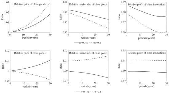
Figure 1.
Income Distribution and Demand-induced Clean Innovations. Note: The legend ‘ = 0.361 relative to = 0.59’ in the three graphs refers to the ratio of the price (market size, and profit) for clean consumer goods under scenarios where the population share of the low-income group is 0.361 and 0.59, respectively ( = 0.59 is the baseline scenario). Other legends follow the same notation.
3.2. Environmental Policy and Transition to Clean Technology
Equation (21) demonstrates that environmental policy is essential for promoting directed clean technology, with its real effects primarily operating through the demand side. Owing to the market power of intermediate firms, the burden of the pollution tax can be fully shifted to consumers through tax-inclusive prices of consumer goods. notably, pollution tax lowers the relative price of clean consumer goods. When the two types of consumer goods are gross substitutes, a lower relative price of clean consumer goods expands their market size. Although the pollution tax ostensibly targets firms producing dirty goods, it actually stimulates innovation by influencing market size. The pollution tax exerts substantial influence on clean innovation by altering the relative prices, market sizes, and profits of clean consumer goods.
Acemoglu et al. and Wang et al. assume identical innovation processes for dirty and clean technologies, causing dirty technologies to monopolize all R&D resources under a laissez-faire equilibrium [4,8,40]. However, once environmental policies intervene, all R&D resources are entirely restricted toward clean technology. Consequently, such models are inadequate for analyzing technological path dependence. A more realistic case is one in which dirty technology declines gradually rather than ceasing immediately following the implementation of environmental policies. Moreover, the presence of path dependence in dirty technology ensures its continued progress even as clean technology advances. To address this issue, the present paper introduces learning-by-doing as the mechanism for dirty technological progress.
We now examine how environmental policies influence the transition to clean technology in the context of demand-induced innovation. Let denote the rate of technological progress in sector s at time . Accordingly, the rate of technological progress in the clean sector at time is given by (Equation (17)), while that in the dirty sector is given by (Equation (18)), where . Given the technological level of sector at time , denoted by , substituting the expressions for and into the respective technological level equations of the two sectors, and , yields the next Equation:
where and represent the initial levels of clean and dirty technologies, respectively, is the concatenated product from period 1 to period , and .
The transition to clean technology is defined as the stage at which the level of clean technology surpasses that of dirty technology, i.e., [4,8]. Equation (22) indicates that two driving forces underpin the transition to clean technology: the initial technology gap and the cumulative gap in market size. the initial technology gap and the cumulative gap in market size . Environmental policies—such as environmental taxes and R&D subsidies—generate a relative price advantage for clean consumer goods and expand their relative market size. Therefore, the stringency of environmental policies directly determines the timing of the transition to clean technology.
The numerical simulations presented in Figure 2 illustrate how varying levels of policy stringency influence both the timing and dynamics of the transition to clean technology. The main findings can be summarized as follows. (i) Under the laissez-faire equilibrium, the path dependence of dirty technology leads to a lower relative price and a larger relative market size for dirty consumer goods, thereby prolonging the time required for clean technology to catch up. (ii) More stringent environmental policies reduce the relative price of clean consumer goods, expand their relative market size, and enhance profit incentives for clean innovation, thereby accelerating the emergence of clean technological transformation.
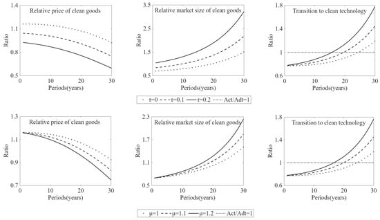
Figure 2.
Environmental Policy, Demand-induced Clean Innovation and Transition to Clean Technology. As in the text,
and
denote pollution tax and R&D subsidy, respectively. The horizontal line, , implies that the clean technology exactly catches up with the dirty technology.
3.3. Environmental Preferences and Transition to Clean Technology
As economic development progresses, environmental awareness and ecological values tend to become more widespread and deeply internalized. In terms of consumption behavior, this evolution is reflected in a higher income elasticity of demand for clean consumer goods relative to polluting goods, implying that the expenditure share of clean goods increases with rising income. A growing body of literature finds that environmental preferences, or public environmental awareness more broadly, play an important role in stimulating clean innovation and facilitating the transition to clean technologies. Some studies even argue that environmental preferences may serve as an effective substitute for formal environmental regulation [57,58].
Environmental preferences can influence the direction of technological change toward cleaner technologies through at least two channels. First, stronger environmental preferences increase consumers’ willingness to pay for clean goods, thereby enhancing the expected profitability of R&D activities directed toward clean technologies [59,60]. Second, heightened environmental preferences can alleviate competitive pressure on firms producing clean goods, encouraging greater investment in the development and adoption of clean technologies [34].
Figure 3 employs numerical simulations to examine the impact of environmental preferences on clean innovation incentives and the transition to clean technology. The results indicate that an increase in the income elasticity of demand for clean consumption goods relative to polluting goods strengthens incentives for clean innovation, thereby accelerating the pace of the transition to clean technology.
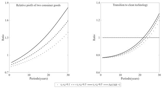
Figure 3.
Income Elasticity, Relative Profitability of Clean Consumption Goods (Relative to Polluting Goods), and the Transition to Clean Technology.
Another channel through which environmental preferences influence the direction of technological change is the elasticity of substitution between clean and polluting consumption goods. Under the representative consumer assumption, Acemoglu et al. and Greaker et al. examine the social welfare losses arising from delayed environmental policy intervention by focusing on the elasticity of substitution between clean and dirty inputs, thereby quantifying the cost of policy delay [8,10]. Following this line of research, the present study adopts comparable parameter values and compares whether scenario (the benchmark case) or scenario (the counterfactual case) generates stronger incentives for clean innovation, thus enabling an earlier transition to clean technology.
Departing from Acemoglu et al. and Greaker et al. this paper analyzes the effect of consumption-good substitution elasticity on transition to clean technology within a framework characterized by income inequality and non-homothetic preferences [8,10]. As shown in Equations (8) and (9), the elasticity of substitution across consumption goods governs household demand for the two types of intermediate goods. Changes in this elasticity therefore alter the consumption structure across income groups, which in turn affects the incentives for technological innovation. Figure 4 presents numerical simulation results that corroborate this mechanism. A higher elasticity of substitution is associated with stronger incentives for clean innovation, thereby accelerating the economy’s transition toward clean technology.
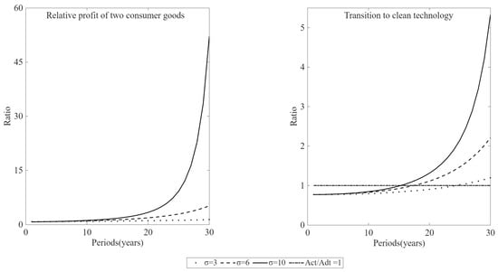
Figure 4.
Income elasticity, the relative profitability of clean (versus polluting) consumption goods, and the transition to clean technology.
4. Discussion
From a dynamic perspective, environmental policy shapes a U-shaped trajectory of environmental quality, and income inequality influences the regulatory effectiveness of such policies throughout this evolutionary process. The U-shaped pattern reflects the dynamic process through which clean technology catches up with and eventually surpasses polluting technology.
(1) The “catch-up” phase of clean technology. Environmental policy redirects innovative resources toward clean technologies, thereby accelerating their rate of technological progress. However, polluting technologies initially retain a technological advantage. As a result, clean technology enters a catch-up phase. During this stage, polluting technologies retain a technological advantage, resulting in higher output of polluting goods and a continued deterioration of environmental quality. (2) The turning point at technological parity. Despite the initial advantage of polluting technologies, the faster rate of progress in clean technologies ensures that they eventually catch up. At this turning point, the two technologies reach parity in terms of technological level or knowledge stock, resulting in comparable outputs of clean and polluting goods. Consequently, the deterioration of environmental quality caused by polluting production reaches its minimum. (3) The transition to clean technology phase. Once clean technologies surpass polluting technologies, their technological advantage becomes increasingly evident. This advantage lowers the relative price of clean consumption goods compared with polluting goods, expands the market share of clean products, and accelerates substitution away from polluting consumption. As the output of polluting goods declines, environmental quality gradually improves.
Owing to the initial advantage of dirty technology, path dependence directs the economy toward the continued use of dirty technology under a laissez-faire equilibrium. Therefore, environmental policies are indispensable for reversing the technological advantage of the dirty sector and facilitating the transition to clean technology. However, under the assumptions of the representative consumer and homothetic preferences, previous models inadequately capture the role of demand-induced innovation in driving the transition to clean technology. Moreover, prior studies have not elucidated how and why income inequality constrains the effectiveness of environmental policies. To address the limitations, this paper incorporates income inequality and non-homothetic preferences into a multi-sectors growth model. In the proposed model, monopolistically competitive intermediate firms weigh both the relative prices and market sizes of consumer goods when making innovation decisions. This suggests that incentives for clean innovations, as well as the dynamics of both technologies, are directly influenced by income inequality. Therefore, environmental policies primarily operate through the demand side, and income inequality exerts a substantial influence on their effectiveness.
4.1. The Population Share of Low-Income Group and the Effectiveness of Environmental Policy
According to the income distribution function (Equation (1)), if the relative per capita income of the low-income group remains constant, a decline in its population share reduces the relative per capita income of the high-income group. This occurs because the fixed total income of the high-income group must be distributed among a larger number of individuals in the high-income groups. An important question thus arises: can a decline in the population share of the low-income group strengthen the effectiveness of environmental policies? Figure 5 illustrates that, under the same stringency of environmental policy (i.e., a pollution tax rate of 0.1 and an R&D subsidy rate of 1.1), a smaller population share of the low-income group both delays the transition to clean technology and weakens its effect on environmental quality improvement.
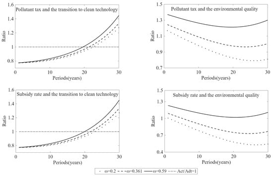
Figure 5.
The population share of the low-income group and the effectiveness of environmental policy.
When the population share of the low-income group decreases, the relative share of high-income consumers correspondingly rises. Meanwhile, the per capita income of the low-income group remains constant, whereas that of the high-income group declines. The increase in innovation profits from a larger high-income population is insufficient to compensate for the profit loss due to the lower per capita consumption of this group. In addition, the per capita consumption of the low-income group remains constant throughout the adjustment process. As a result, a reduction in the population share of the low-income group may postpone the transition to clean technology and provide only limited improvements in environmental quality.
4.2. The per Capita Income of the Low-Income Group and the Effectiveness of Environmental Policy
A reduction in income inequality can alternatively be analyzed through an increase in the relative per capita income of the low-income group. Equation (1) shows that, when the population share of the low-income group remains constant, an increase in their relative per capita income reduces the per capita income of the high-income group, thereby leading to a more equitable income distribution. This mechanism is critical because differences in the marginal propensity to consume across income groups shapes the overall consumption structure, which in turn influences incentives for clean innovation. Figure 6 shows the effectiveness of environmental policies (specifically, a pollution tax rate of 0.1 and an R&D subsidy rate of 1.1) across various per capita income levels of the low-income group.
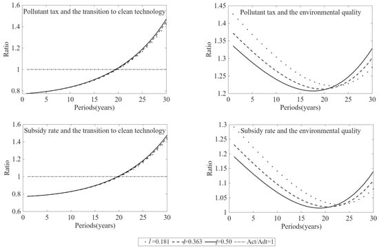
Figure 6.
The per capita income of the low-income group and the effectiveness of environmental policy.
Due to differences in the marginal propensity to consume between high- and low-income groups, an increase in the per capita income of the low-income group partially offsets the innovation incentives originating from both groups. Nevertheless, the net effect contributes to promoting the transition to clean technology. Furthermore, increasing the per capita income of the low-income group not only shifts the turning point of the ‘U-shaped’ trajectory of environmental quality earlier but also results in a substantial enhancement of overall environmental quality. Therefore, a higher per capita income among the low-income population plays a crucial role in stimulating the transition to clean technology and improving environmental quality.
4.3. Income Inequality and Differences in the Effectiveness of Environmental Policy
Exploring the differential effectiveness of environmental policies in facilitating the transition to clean technology constitutes another important line of inquiry. For example, Aghion et al. mphasized the role of pollution tax, whereas other studies contend that R&D subsidies play a more decisive role [7,8,10]. This raises the question of whether income inequality can offer new insights into the relative effectiveness of different environmental policy instruments. As shown in Figure 3 and Figure 4, no substantial differences appear to exist between a pollution tax of 0.1 and an R&D subsidy of 1.1 in advancing the transition to clean technology. However, compared with the impact of the R&D subsidies on environmental quality, the pollution tax not only drastically enhances environmental quality but also accelerates the timing of the ‘turning point’ in its quality. This divergence arises because the pollution taxes and R&D subsidies emphasize distinct mechanisms. Specifically, the pollution tax penalizes the production and consumption of dirty goods, thereby directly mitigating environmental degradation and speeds up the transition to clean technology via demand-induced innovation. In addition, coupling between macro-level development strategies and technological innovation systems significantly influences the availability of finance and the diffusion pathways of green innovation [61].
4.4. Income Inequality, Environmental Policy and Social Welfare
The fundamental objective of mitigating environmental degradation and climate change is to improve social welfare by satisfying society’s demand for a high-quality ecological environment. However, environmental policies often distort private-sector behavior in consumption, production, and research and development, implying that such policies may generate welfare effects during the process of promoting transition to clean technology. Unlike Acemoglu et al., who measure social welfare using final consumption goods, this study constructs a social welfare function based on Equations (2) and (4), which explicitly captures how environmental policies affect welfare through substitution between clean and polluting consumption goods [8].
To evaluate welfare effects, social welfare under the free-market equilibrium without environmental policy intervention is taken as the benchmark. We then compute the ratio of social welfare under environmental policy to that under the free-market equilibrium. A ratio below one indicates that the policy induces a welfare loss relative to the free-market outcome, whereas a ratio above one indicates a welfare gain. Figure 7 illustrates the welfare effects of environmental policies under income inequality.
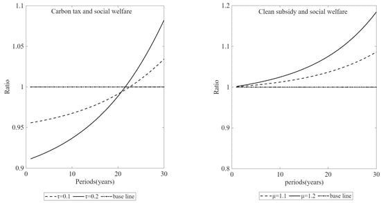
Figure 7.
Environmental policy and social welfare.
Figure 7 reveals several key patterns. First, carbon taxes generate welfare losses in the early stages of implementation, and stricter carbon taxes lead to larger initial welfare losses. Second, after a certain period, carbon taxes yield welfare gains, with more stringent carbon taxes producing higher long-term welfare. Third, even in the initial phase, green innovation subsidies deliver higher social welfare than the free-market equilibrium.
The welfare effects of carbon taxes arise because they directly increase the relative price of polluting consumption goods. In the early stage of implementation, corresponding to the phase in which clean technology is catching up with polluting technology, the decline in real income dominates, leading to welfare losses. Once the transition to clean technology is achieved, clean consumption goods become relatively cheaper than polluting goods prior to the carbon tax. At this stage, the substitution effect outweighs the income effect associated with reduced real income, and the environmental quality attributes of clean goods further enhance utility, resulting in welfare improvements.
In contrast, green innovation subsidies do not directly distort consumption behavior and therefore do not generate initial welfare losses. As the subsidy promotes clean innovation and raises the level of clean technology, the relative price of clean consumption goods continues to decline, leading to sustained improvements in social welfare over time.
5. Conclusions
Income inequality and environmental degradation have emerged as pressing global challenges, yet the intrinsic linkage between them has received insufficient scholarly attention. On the one hand, income inequality influences the direction of technical change and the effectiveness of environmental policies. On the other hand, the key to mitigating environmental degradation lies in facilitating the transition from dirty to clean technologies [7]. Nevertheless, existing theories of directed technical change largely overlook these interconnections between income inequality and environmental quality. To address these shortcomings, the present paper introduces several important improvements to the existing literature. On the demand side, income distribution and non-homothetic CES preferences are incorporated to capture how income inequality shapes consumer composition and thereby affects the direction of technical change. On the supply side, the model assumes asymmetric technological changes between dirty and clean sectors, thereby ensuring path dependence and capturing the ‘U-shaped’ evolution of environmental quality. Building on these extensions, a multi-sector model of directed technical change is developed to examine how income inequality and environmental policies jointly influence the transition to clean technology. The main results are as follows.
First, consumer composition plays a crucial role in driving the transition to clean technology and improving environmental quality. Under non-homothetic CES preferences, income inequality influences the direction of technological change via innovation incentives. On the one hand, income inequality functions as a wedge that determines consumer composition or the relative market sizes of the two types of consumer goods. On the other hand, consumer composition affects the growth rates of both dirty and clean technologies through learning-by-doing and demand-induced innovation, respectively. Overall, income distribution shapes incentives for clean innovation and directly influences the transition to clean technology. Second, income inequality constitutes a critical constraint on the effectiveness of environmental policies. When the two types of consumer goods are gross substitutes, their prices are inversely related to their respective market sizes. The primary function of environmental policies is to reverse the initial advantage of dirty technology and thereby expand the market size of clean consumer goods. Furthermore, income inequality governs and constrains the relative market sizes of the two types of consumer goods. Therefore, income distribution exerts a significant impact on the effectiveness of environmental policies.
Third, introducing asymmetric approaches to technological change in the dirty and clean sectors not only captures path dependence but also explains the dynamic ‘U-shaped’ trajectory of environmental quality. In contrast, symmetric approaches to technological change omit path dependence in clean technology under the laissez-faire equilibrium and fail to capture the persistence of dirty technology under environmental policies. However, when technological progress arises from learning-by-doing and demand-induced innovation, the growth rates of the two technologies evolve simultaneously, yet depend on their respective market sizes. The transition to clean technology unfolds in two stages: clean technology first catches up with and then surpasses dirty technology. During this process, environmental quality follows a ‘U-shaped’ trajectory, initially deteriorating and subsequently improving.
From a policy perspective, the results suggest that income distribution may play an important mediating role in the transition toward clean technology by shaping demand-side innovation incentives. Policies that improve the relative income position of lower-income groups could, in principle, expand the market size for clean consumption and thereby strengthen demand-induced innovation. In this sense, redistributive measures combined with instruments that support green consumption may indirectly reinforce the effectiveness of environmental regulation by alleviating demand-side constraints associated with income inequality. Such interactions are consistent with the implications of non-homothetic CES preferences, under which market size rather than average income drives innovation incentives, and may help advance the turning point of the U-shaped environmental quality trajectory identified in the model.
The findings also indicate that income inequality can limit the effectiveness of environmental policies when these rely on a single instrument. A more diversified policy mix may therefore be more effective. For example, pollution taxes can alter relative prices in favor of clean goods, while targeted subsidies for clean innovation or consumption can help mitigate distributional side effects. Given the asymmetric mechanisms of technological change, with clean technology driven primarily by demand-induced innovation and dirty technology characterized by learning-by-doing, a gradual and sequenced policy approach appears particularly relevant. Such a framework may allow clean technologies to progressively improve their market position without generating excessive short-term welfare losses, especially for lower-income households.
More broadly, the analysis highlights the importance of coordinating supply- and demand-side policies in the presence of technological path dependence. On the supply side, measures that support incremental improvements in clean technology quality may help sustain innovation incentives over time. On the demand side, policies that broaden access to clean products can contribute to market expansion while improving distributional outcomes. At the same time, a gradual adjustment of polluting technologies, rather than abrupt displacement, may reduce transition costs and enhance policy acceptability. Taken together, these considerations underscore that accounting for income heterogeneity is not only relevant for equity concerns but may also improve the long-run efficiency and stability of the transition to clean technology.
Several limitations of this study should be acknowledged. First, income distribution is modeled using two representative income groups. This stylized representation allows for clear intuition and analytical tractability, but it inevitably abstracts from the continuous and more complex structure of real-world income distributions. Future research could extend the framework by incorporating a richer income distribution to better capture heterogeneity across households. Second, some key parameters that govern the central mechanisms of the model, such as the income elasticities of clean and dirty consumption, are calibrated based on influential studies in the literature and examined through sensitivity analysis. While this approach is standard in theoretical work, the availability of suitable micro-level data would allow for structural estimation of these parameters, which could substantially enhance the model’s empirical relevance. Finally, the model assumes infinitely divisible consumption goods, a common feature in directed technical change frameworks. However, parts of the demand-induced innovation literature adopt an indivisible consumption assumption, where consumption decisions are discrete. Under such settings, households’ willingness to pay may play a more prominent role in firms’ pricing and innovation incentives. Due to computational complexity and space constraints, this extension is not explored here and is left for future research.
Author Contributions
Conceptualization, H.X.; methodology, Y.C.; formal analysis, H.X.; investigation, Y.C.; data curation, Y.C.; writing—original draft preparation, H.X.; writing—review and editing, W.Z.; visualization, Y.C.; supervision, H.X.; project administration, W.Z. All authors have read and agreed to the published version of the manuscript.
Funding
This article is supported by Jilin Provincial Social Science Fund Key Project (2025A18): Research on the Important Mission of Jilin Province in Safeguarding China’s ‘Five Major Securities’. The funder of this project is: “Jilin Provincial Philosophy and Social Sciences Planning Fund Office”.
Institutional Review Board Statement
Not applicable.
Informed Consent Statement
Not applicable.
Data Availability Statement
The data presented in this study are available on request from the corresponding author. Meanwhile, they are openly available in Figshare at https://doi.org/10.6084/m9.figshare.30486911.v1.
Conflicts of Interest
The authors declare no conflict of interest.
Appendix A

Table A1.
Calibration.
Table A1.
Calibration.
| Parameter | Description | Value |
|---|---|---|
| the income elasticity of clean consumer goods | 1.1 | |
| the income elasticity of dirty consumer goods | 1 | |
| the elasticity of substitution | 3 | |
| the time discount factor | 0.99 | |
| the importance parameter of dirty consumer goods | 0.5 | |
| the importance parameter of clean consumer goods | 0.5 | |
| the distribution parameter | 0.8 | |
| the output elasticity of capital | 0.43 | |
| the depreciation rate of capital | 0.05 | |
| the rung on the quality ladder | 0.1 | |
| the initial gap between dirty and clean technology | 1.3 | |
| the population proportion of low-income group | 0.59 | |
| the relative per income of the low-income group | 0.363 | |
| the innovation elasticity of research and development expenditure | 0.5 | |
| the indicator parameter | 1.128 | |
| the knowledge spillover parameter | 0.12 | |
| the speed of learning | 0.047 | |
| the rarity of pollution degradation | 0.75 | |
| the rate of pollution emission | 2.62 | |
| the initial environmental quality | 2.6 |
Table A2.
Variables.
Table A2.
Variables.
| Parameter | Description | Nature |
|---|---|---|
| the relative per income of the low-income group | exogenous | |
| the relative per income of the high-income group | exogenous | |
| the population proportion of low-income group | exogenous | |
| the quantities of clean intermediate consumer goods | endogenous | |
| the quantities of dirty intermediate consumer goods | endogenous | |
| clean consumer goods | endogenous | |
| dirty consumer goods | endogenous | |
| the market size of the intermediate consumer goods in the clean sector | endogenous | |
| the market size of the intermediate consumer goods in the dirty sector | endogenous | |
| environmental attributes of clean intermediate consumer goods | endogenous | |
| environmental attributes of dirty intermediate consumer goods | endogenous | |
| the real consumption index of consumer | endogenous | |
| the exact price index of consumer | endogenous | |
| consumption expenditure of consumer | endogenous | |
| capital stock of consumer | endogenous | |
| the income inequality wedge | endogenous | |
| the total income or per capita income of the economy | endogenous | |
| the rental rate of capital | endogenous | |
| the wage rate | endogenous | |
| monopoly profit of the clean intermediate consumer good | endogenous | |
| monopoly profit of the dirty intermediate consumer good | endogenous | |
| R&D expenditure of the dirty intermediate consumer good | endogenous | |
| the probability of successful innovation for clean intermediate goods | endogenous | |
| the growth rate of the clean consumer goods | endogenous | |
| the growth rate of the dirty consumer goods | endogenous | |
| the stock of clean technology | endogenous | |
| the stock of dirty technology | endogenous | |
| environmental quality | endogenous | |
| pollution stock | endogenous |
Appendix B
This section conducts a sensitivity analysis of several key parameters in the theoretical model to assess its robustness. As shown in Figure A1, the main results of the model are robust to variations in parameter values.

Figure A1.
Robustness Checks. Note: Because the step size of the quality ladder does not affect the rate of technological progress, and coincide.
References
- Popp, D. ENTICE: Endogenous technological change in the DICE model of global warming. J. Environ. Econ. Manag. 2004, 48, 742–768. [Google Scholar] [CrossRef]
- Popp, D. Environmental policy and innovation: A decade of research. Int. Rev. Environ. Resour. Econ. 2019, 13, 265–337. [Google Scholar] [CrossRef]
- Johnstone, N.; Haščič, I.; Popp, D. Renewable Energy Policies and Technological Innovation: Evidence Based on Patent Counts. Environ. Resour. Econ. 2010, 45, 133–155. [Google Scholar] [CrossRef]
- Acemoglu, D.; Akcigit, U.; Hanley, D.; Kerr, W. Transition to Clean Technology. J. Political Econ. 2016, 124, 52–104. [Google Scholar] [CrossRef]
- Greaker, M.; Popp, D. Environmental Economics, Regulation, and Innovation. Working Paper NO. 30415, NBER, Cambridge, MA, USA, 2022. [Google Scholar]
- Ramírez-Gutiérrez, A.G.; Solano García, P.; Morales Matamoros, O.; Moreno Escobar, J.J.; Tejeida-Padilla, R. Systems Approach for the Adoption of New Technologies in Enterprises. Systems 2023, 11, 494. [Google Scholar] [CrossRef]
- Aghion, P.; Dechezleprêtre, A.; Hémous, D.; Alp, H.; Bloom, N.; Kerr, W. Innovation, Reallocation, and Growth. Am. Econ. Rev. 2018, 108, 3450–3491. [Google Scholar] [CrossRef]
- Acemoglu, D.; Aghion, P.; Bursztyn, L.; Hemous, D. The Environment and Directed Technical Change. Am. Econ. Rev. 2012, 102, 131–166. [Google Scholar] [CrossRef]
- Foellmi, R.; Zweimüller, J. Income Distribution and Demand-Induced Innovations. Rev. Econ. Stud. 2006, 73, 941–960. [Google Scholar] [CrossRef]
- Greaker, M.; Heggedal, T.R.; Rosendahl, K.E. Environmental policy and the direction of technological change. Scand. J. Econ. 2018, 120, 1100–1138. [Google Scholar] [CrossRef]
- Scruggs, L.A. Political and economic inequality and the environment. Ecol. Econ. 1998, 26, 259–275. [Google Scholar] [CrossRef]
- Ravallion, M.; Heil, M.; Jalan, J. Carbon Emissions and Income Inequality. Oxf. Econ. Pap. 2000, 52, 651–669. [Google Scholar] [CrossRef]
- Heerink, N.; Mulatu, A.; Bulte, E. Income inequality and the environment: Aggregation bias in environmental Kuznets curves. Ecol. Econ. 2001, 38, 359–367. [Google Scholar] [CrossRef]
- Boyce, J. Inequality as a cause of environmental degradation. Ecol. Econ. 1994, 11, 169–178. [Google Scholar] [CrossRef]
- Torras, M.; Boyce, J.K. Income, inequality, and pollution: A reassessment of the environmental Kuznets Curve. Ecol. Econ. 1998, 25, 147–160. [Google Scholar] [CrossRef]
- Magnani, E. The Environmental Kuznets Curve, environmental protection policy and income distribution. Ecol. Econ. 2000, 32, 431–443. [Google Scholar] [CrossRef]
- Boyce, J. Income inequality and environmental quality: Are they linked? Ecol. Econ. 2007, 62, 601–609. [Google Scholar]
- Kempf, H.; Rossignol, S. Is Inequality Harmful for the Environment in a Growing Economy. Econ. Politics 2007, 19, 53–71. [Google Scholar] [CrossRef]
- Vona, F.; Patriarca, F. Income inequality and the development of environmental technologies. Ecol. Econ. 2011, 70, 2201–2213. [Google Scholar] [CrossRef]
- Matsuyama, K. The Rise of Mass Consumption Societies. J. Political Econ. 2002, 110, 1035–1070. [Google Scholar] [CrossRef]
- Gamidullaeva, L.; Shmeleva, N.; Tolstykh, T.; Guseva, T.; Panova, S. The Complex Approach to Environmental and Technological Project Management to Enhance the Sustainability of Industrial Systems. Systems 2024, 12, 261. [Google Scholar] [CrossRef]
- Bovenberg, L.; Smulders, S. Environmental quality and pollution-augmenting technological change in a two-sector endogenous growth model. J. Public Econ. 1995, 57, 369–391. [Google Scholar] [CrossRef]
- Stokey, N.L. Are There Limits to Growth? Int. Econ. Rev. 1998, 39, 1–31. [Google Scholar] [CrossRef]
- Van der Zwaan, B. Learning-by-doing and the economics of climate change. Energy Econ. 2002, 24, 273–291. [Google Scholar]
- Popp, D. Induced innovation and energy prices. Am. Econ. Rev. 2002, 92, 160–180. [Google Scholar] [CrossRef]
- Erikson, R. Income inequality and environmental policy. Scand. J. Econ. 2015, 117, 1243–1267. [Google Scholar]
- Drupp, M.A.; Kornek, U.; Meya, J.N.; Sager, L. The Economics of Inequality and the Environment. J. Econ. Lit. 2025, 63, 840–874. [Google Scholar] [CrossRef]
- Stiglitz, J.E. The Price of Inequality: How Today’s Divided Society Endangers Our Future; W.W. Norton & Company: New York, NY, USA, 2012. [Google Scholar]
- Roca, J. Do Individual Preferences Explain the Environmental Kuznets Curve? Ecol. Econ. 2003, 45, 3–10. [Google Scholar] [CrossRef]
- Kichko, S.; Picard, P.M. On the effects of income heterogeneity in monopolistically competitive markets. J. Int. Econ. 2023, 143, 103759. [Google Scholar] [CrossRef]
- Kaufmann, M.; Andre, P.; Kőszegi, B. Understanding Markets with Socially Responsible Consumers. Q. J. Econ. 2024, 139, 1989–2035. [Google Scholar] [CrossRef]
- Blanchard, O.; Gollier, C.; Tirole, J. The Portfolio of Economic Policies Needed to Fight Climate Change. Annu. Rev. Econ. 2023, 15, 689–722. [Google Scholar] [CrossRef]
- Lebedev, V.; Miroshnichenko, D.; Pyshyev, S.; Kohut, A. Study of Hybrid Humic Acids Modification of Environmentally Safe Biodegradable Films Based on Hydroxypropyl Methyl Cellulose. Chem. Chem. Technol. 2023, 17, 357–364. [Google Scholar] [CrossRef]
- Aghion, P.; Bénabou, R.; Martin, R.; Roulet, A. Environmental preferences and technological choices: Is market competition clean or dirty? Am. Econ. Rev. Insights 2023, 5, 1–20. [Google Scholar] [CrossRef]
- Acemoglu, D.; Aghion, P.; Barrage, L.; Hémous, D. Climate Change, Directed Innovation, and Energy Transition: The Long-Run Consequences of the Shale Gas Revolution. NBER Working Paper 31657, National Bureau of Economic Research, Cambridge, MA, USA, 2024. [Google Scholar]
- Hémous, D.; Olsen, M. Directed Technical Change in Labor and Environmental Economics. Annu. Rev. Econ. 2021, 13, 571–597. [Google Scholar] [CrossRef]
- Zweimüller, J. Schumpeterian entrepreneurs meet Engel’s law: The impact of inequality on innovation-driven growth. J. Econ. Growth 2000, 5, 185–206. [Google Scholar] [CrossRef]
- Ling, S.; Guoqiang, T. Income inequality, urbanization and economic growth: A demand-side analysis. Econ. Res. J. 2009, 44, 17–29. [Google Scholar]
- Aovales, A.; Esther, F.; Jesus, R. Economic Growth: Theory and Numerical Solution Methods; Springer: Berlin/Heidelberg, Germany, 2014. [Google Scholar]
- Wang, L.; Wang, H.; Dong, Z. Policy Conditions for Compatibility between Economic Growth and Environmental Quality: A Test of Policy Bias Effects from the Perspective of the Direction of Environmental Technological Progress. J. Manag. World 2020, 36, 38–59. [Google Scholar]
- Acemoglu, D. Introduction to Modern Economic Growth; Princeton University Press: Princeton, NJ, USA, 2009. [Google Scholar]
- Arrow, K.J. The Economic Implications of Learning by Doing. Rev. Econ. Stud. 1962, 29, 155–173. [Google Scholar] [CrossRef]
- Romer, P.M. Increasing Returns and Long-Run Growth. J. Political Econ. 1986, 94, 1002–1037. [Google Scholar] [CrossRef]
- Aghion, P.; Howitt, P. Endogenous Growth Theory; MIT Press: Cambridge, MA, USA, 1998. [Google Scholar]
- Aghion, P.; Howitt, P. The Economics of Growth; MIT Press: Cambridge, MA, USA, 2009. [Google Scholar]
- Barro, R.J.; Sala-i-Martin, X. Economic Growth; The MIT Press: Cambridge, MA, USA, 2004. [Google Scholar]
- Huang, M.; Lin, S. Pollution Damage, Environmental Management and Sustainable Economic Growth: Based on the Analysis of a Five-Department Endogenous Growth Model. Econ. Res. J. 2013, 48, 30–41. [Google Scholar]
- Fan, Q. Environmental Regulation, Income Distribution Imbalance and Government Compensation Mechanisms. Econ. Res. J. 2018, 53, 14–27. [Google Scholar]
- Heutel, G. How Should Environmental Policy Respond to Business Cycles? Optimal Policy Under Persistent Productivity Shocks. Rev. Econ. Dyn. 2012, 15, 244–264. [Google Scholar] [CrossRef]
- Krisrom, B.; Riera, P. Is the Income Elasticity of Environmental Improvements Less than One? Environ. Resour. Econ. 1996, 7, 45–55. [Google Scholar] [CrossRef]
- Ghalwash, T.M. Demand for Environmental Quality: An Empirical Analysis of Consumer Behavior in Sweden. Environ. Resour. Econ. 2008, 41, 71–87. [Google Scholar] [CrossRef]
- Comin, D.; Lashkari, D.; Mestieri, M. Structural Change with Long-Run Income and Price Effects. Econometrica 2021, 89, 311–374. [Google Scholar] [CrossRef]
- Duernecker, G.; Herrendorf, B.; Valentinyi, A. Structural Change Within the Service Sector and the Future of Baumol’s Disease. J. Eur. Econ. Assoc. 2024, 22, 428–473. [Google Scholar] [CrossRef]
- Wang, W.; Xian, J. Population Aging, Education Financing Patterns and Economic Growth in China. Econ. Res. J. 2020, 55, 46–63. [Google Scholar]
- Cai, Y.; Fu, Y. The Technical and Structural Effects of TFP Growth: Measurement and Decomposition Based on China’s Macro and Sector Data. Econ. Res. J. 2017, 52, 72–88. [Google Scholar]
- Foellmi, R.; Zweimüller, J. Is inequality harmful for innovation and growth? Price versus market size effects. J. Evol. Econ. 2017, 27, 359–378. [Google Scholar] [CrossRef]
- Lambertini, L. Green innovation and market power. Annu. Rev. Resour. Econ. 2017, 9, 231–252. [Google Scholar] [CrossRef]
- Castro-Santa, J.; Drews, S.; van den Bergh, J. Nudging low-carbon consumption through advertising and social norms. J. Behav. Exp. Econ. 2023, 104, 102–123. [Google Scholar] [CrossRef]
- Rizzati, M.; Ciola, E.; Turco, E.; Bazzana, D.; Vergalli, S. Beyond Green Preferences: Alternative Pathways to Net-Zero Emissions in the MATRIX Model; Working Paper No. 03.2024; Fondazione Eni Enrico Mattei (FEEM): Milano, Italy, 2024. [Google Scholar]
- Biswas, A.; Roy, M. Leveraging factors for sustained green consumption behavior based on consumption value perceptions: Testing the structural model. J. Clean. Prod. 2015, 95, 332–340. [Google Scholar] [CrossRef]
- Lv, S.; Zhao, S.; Liu, H. Research on the Coupling Between the Double Cycle Mode and Technological Innovation Systems: Empirical Evidence from Data Envelopment Analysis and Coupled Coordination. Systems 2022, 10, 62. [Google Scholar] [CrossRef]
Disclaimer/Publisher’s Note: The statements, opinions and data contained in all publications are solely those of the individual author(s) and contributor(s) and not of MDPI and/or the editor(s). MDPI and/or the editor(s) disclaim responsibility for any injury to people or property resulting from any ideas, methods, instructions or products referred to in the content. |
© 2025 by the authors. Licensee MDPI, Basel, Switzerland. This article is an open access article distributed under the terms and conditions of the Creative Commons Attribution (CC BY) license.