Abstract
Weather change, as a physical risk factor of climate change, increasingly impacts the energy market. This paper investigates China’s major energy futures using a QVAR framework to analyze spillover effects under different market conditions, addressing mean-model limitations. It also reveals state-dependent weather impacts on spillovers, providing physical climate risk evidence. The results show the following: (1) Spillover effects intensify under extreme conditions, with crude oil and fuel oil as main transmitters, and methanol and coking coal as key recipients. Coking coal shows a stronger spillover absorption capacity under extreme conditions. (2) The Total Spillover Index (TSI) displays significant time-varying feature and sensitivity to external shocks, with heightened asymmetry and complexity in extreme markets. (3) Weather change significantly affects spillovers of China’s energy futures, with temperature, cooling and heating loads, and precipitation showing different impacts on TSI across market conditions. These findings provide references for energy finance regulation and risk early warning under climate change conditions.
1. Introduction
Climate change has triggered severe turbulence and increased risks in the global energy market, posing greater challenges and uncertainties for market regulators and investors [1,2]. According to the “Global Risk Report 2024”, extreme weather has been identified as one of the most likely global risk factors and it is expected to become one of the main threats to global stability and security in the next decade. This presents severe challenges to energy production, supply, and price stability.
In China, fossil fuels such as coal and oil still dominate the primary energy mix, but under the “dual-carbon” targets, the energy structure is shifting toward low-carbon and diversification [3,4]. This has spurred the rapid expansion of new energy industry, particularly the expansion of the new energy and lithium-ion battery sectors [5,6,7]. As a key financial derivative, energy futures play a core role in risk management and resource allocation and have become a crucial bridge connecting the real economy and the financial market [8]. As the world’s largest energy consumer, China has witnessed a continuous expansion of its energy futures market [9]. Shanghai crude oil futures have ranked as the third-largest crude oil contract globally, following Brent and WTI [10]. China’s energy market not only has a key impact on the domestic economy but also brings profound fluctuations to the global energy landscape [11,12]. Therefore, studying China’s energy futures market holds significant theoretical value and practical significance.
As the financial characteristics of energy commodities become increasingly pronounced, the operation of the energy market is also facing multiple external challenges [13,14,15]. Meanwhile, as climate change intensifies, the risks it brings are gradually emerging. Existing studies show that climate risk is increasingly becoming a key factor influencing the energy market [16,17]. Climate risks are typically classified into physical climate risks (PCR) and transition climate risks (TCR) [18]. Among these, PCR, referring to the direct impact caused by climate change, is one of the most critical types of risk [19,20]. The energy market is highly sensitive to PCR, which is reflected in several key aspects: Firstly, changes in climate patterns directly reshape the structure of energy supply and demand, thereby disrupting the market pricing mechanism [21,22]; Secondly, extreme climate events can damage infrastructure, increase maintenance and production costs, and have a profound impact on the operation of the industry [23]; Finally, climate change can also influence investors’ risk preferences and market expectations, leading to fluctuations in energy asset prices and even triggering shifts in market sentiment [24,25].
However, most studies on the impact of climate change on markets tend to focus on indirect variables to capture climate risk, such as climate policy uncertainty indices or news-based indices derived from text analysis [26,27,28]. While these approaches can partly reflect market expectations and policy responses to climate change, they are still insufficient in capturing physical risks. In contrast, recent studies on PCR highlight the critical role of “direct weather variables” in explaining energy price dynamics and the substantial influence of weather conditions on market co-movements. In fact, weather change, as the most direct and observable manifestation of climate change, can more accurately reflect the influence of PCR on the market and the potential transmission paths [29,30].
Given this context, incorporating weather variables as direct indicators of PCR is essential. National-level meteorological data capture the systemic impact of climate change on China’s energy futures, which are traded on nationwide exchanges with unified pricing mechanisms. Moreover, differences in industrial chain positioning and demand elasticity lead to heterogeneous responses of energy products to weather shocks, potentially reshaping risk transmission and spillover structures across markets. Therefore, a weather-based perspective provides a valuable approach to understanding how PCR affects systemic risk spillovers and energy market stability under climate change.
In view of this, researchers have started to pay increasing attention to the potential effects of weather change on financial markets. Relevant literature shows that weather change is significantly associated with market price fluctuations, asset returns, and investor sentiment, and they exert considerable influence in both financial and energy markets [30,31]. Meanwhile, many achievements have been made in the research on market spillovers. Traditional factors such as geopolitical risks, fluctuations in international oil prices, and economic policy uncertainties have been widely confirmed to trigger risk contagion and spillovers among assets [32,33,34]. However, although weather change is a key manifestation of PCR, systematic research on how weather factors impact spillovers of energy markets remains limited. Therefore, investigating the impact of weather change on energy market spillovers can help fill this gap in the literature.
In terms of research methodology, existing literature mainly employs GARCH-type models [35], DY [36] and BK [37] spillover indices, as well as approaches that integrate these with time-varying parameter vector autoregression (TVP-VAR) models [38,39] to examine spillovers among markets. While these methods offer certain advantages in capturing risk transfer across different markets and frequency ranges, they rely on conditional mean estimates and mainly reflect average spillovers in normal market scenarios. As a result, they are limited in revealing the heterogeneity of spillover effects under different market conditions, such as extreme conditions. To address this, Ando et al. [40] proposed a quantile-based spillover analysis framework by combining the Quantile Vector Autoregression (QVAR) model with the DY spillover approach. The QVAR model has also been widely applied in broader commodity and energy markets, where it demonstrates strong robustness to tail risks and extreme shocks and provides more accurate spillover estimates [41,42,43]. These applications further support the suitability of the QVAR framework for analyzing heterogeneous spillover dynamics.
Based on the above considerations, this paper systematically examines the characteristics of systemic risk spillover effects of China’s energy futures market and their relationship with weather change. Firstly, this paper selects six major energy futures, namely crude oil (SC), fuel oil (FU), coking coal (CC), coke (CK), bitumen (BU), and methanol (MA), as the research objects, and constructs the QVAR-DY model to explore the spillover effects among energy futures under different market conditions. Second, we employ regression models to explore the impact of weather factors such as temperature (TE), cooling degree days (CDD), heating degree days (HDD), and total precipitation (TP) on total spillovers across different market conditions (the research framework is shown in Figure 1). The main marginal contributions of this paper are reflected in the following aspects: (1) This study focuses on China’s emerging energy futures market. Unlike most existing studies that examine climate-related impacts in developed economies [44,45], the Chinese case also provides transferable insights for other major energy-consuming developing countries, including India, Indonesia, Malaysia, and South Africa, that share similar fossil-fuel dependence, growing derivatives markets, and rising exposure to extreme weather. (2) This paper adopts the Quantile Vector Autoregression (QVAR) approach to capture spillovers characteristics among China’s energy futures markets under different conditions, including both normal and extreme conditions. The QVAR method overcomes the limitations of traditional mean-based models and allows for a more comprehensive depiction of spillover effects and their evolution across market conditions, thus improving the ability to identify extreme market risks. (3) Compared with the commonly used climate policy uncertainty indices or text-based climate risk indicators in existing research, this paper introduces weather change factors that directly measure PCR. From a “weather perspective,” it reveals the influence mechanism of weather change on the spillovers in the energy futures under the background of frequent extreme weather events.

Figure 1.
Research framework.
The structure of this paper is arranged as follows: Section 2 introduces the models and methods used in the empirical analysis. Section 3 presents the data employed in the study. Section 4 discusses the empirical results. Section 5 provides the main conclusions, policy recommendations and limitations.
2. Methodology
2.1. QVAR Spillover Index
Ando et al. [40] developed a QVAR-based spillover index building on the spillover framework [36], enabling the calculation of spillover effects across markets at different quantile levels. This allows for the measurement of tail risk spillovers. To clearly demonstrate the advantages of the QVAR model over mainstream spillover models such as TVP-VAR and GARCH, this paper compares the three models, with the specific results shown in Table A1 (see Appendix A).
This study selects the 0.05, 0.50, and 0.95 quantiles because they form the standard combination for capturing downside tail risk, normal market conditions, and upside tail risk in financial markets. These quantiles are fully consistent with the theoretical design of the QVAR model and match the pronounced fat-tail characteristics of China’s energy futures, thereby maximizing the ability to reveal the state-dependent heterogeneity of spillover effects. First, a QVAR() model is constructed as follows:
where and are dimensional vectors of endogenous variables, represents the quantile level, is the lag order of the model, is the dimensional conditional mean vector, is the dimensional coefficient matrix, and is the dimensional error term matrix.
Then, the QVAR() model is transformed into an infinite-order Quantile Vector Moving Average (QVMA) representation:
Based on the Generalized Forecast Error Variance Decomposition (GFEVD) method, the impact of market on market can be expressed as:
where denotes a selection vector with 1 at position and 0 in all other positions. Next, Equation (3) is standardized as follows:
where and . represents the impact from vector on the forecast error variance of vector at horizon , which can be used to measure the spillover intensity from vector to vector . Next, based on the spillover index framework developed by Diebold and Yılmaz [36], we compute the risk spillover index across different quantile levels.
According to the DY spillover index, the total spillover index is defined as:
The directional spillover index and the net spillover index can be expressed as follows:
Spillovers transmitted to others (To):
Spillovers received from others (From):
Net spillover index (NET):
2.2. Regression Model for the Impact of Weather Change on Spillover Effects of Energy Futures
To systematically examine the direction and magnitude of the influence of weather change on the spillover effects of China’s energy futures market, this paper constructs the following regression model:
where represents the total spillover index at quantile on day , is the intercept term, indicates the direction and magnitude of the impact of weather factors, captures the effect of control variables; and denotes the error term.
The core explanatory variables include temperature (TE), cooling degree days (CDD), heating degree days (HDD), and total precipitation (TP). These variables are selected based on the following considerations: Firstly, TE is the most fundamental and widely used meteorological variable, which directly affects the energy consumption structure and has a significant effect on the energy market [46]. Secondly, CDD and HDD, as indicators of cooling and heating loads, offer a more precise reflection of extreme temperature effects on energy consumption, thereby influencing the spillover structure in the energy market [47]. Finally, TP indirectly affects energy consumption and supply efficiency, potentially triggering fluctuations in the energy market [48]. The control variables include geopolitical risk (GPR), Chicago Board Options Exchange (CBOE) volatility index (VIX), CBOE crude oil volatility (OVX), the USD to RMB exchange rate (Rate), and the CSI 300 index (CSI300). The selection of these control variables is based on the following considerations: Firstly, GPR serves as a key external shock influencing the structure of energy supply and demand. It increases market uncertainty and volatility, thereby significantly impacting the spillovers of energy futures market [49,50,51]. Secondly, VIX and OVX are widely used indicators measuring overall market panic and crude oil market volatility, respectively, and are commonly employed to capture spillover effects among markets [33,42]. Additionally, previous studies have shown that volatility in exchange rates exerts a notable influence on the energy market [52], and there is a close interconnection between the stock market and the energy market [53,54]. Changes in the stock market can also transmit to the energy futures market, influencing the pathways of systemic risk diffusion. Furthermore, to eliminate the influence of differing units of measurement, the TSI, GPR, VIX, OVX, Rate, and CSI300 variables are all log-transformed.
2.3. Return Calculation
The formula for the energy futures return is calculated as follows:
where denotes the return on day , and represent the closing prices on day and day , respectively.
3. Data
This study selects six major energy futures as research subjects: crude oil (SC), fuel oil (FU), coking coal (CC), coke (CK), bitumen (BU), and methanol (MA). According to the Market Annual Report of the Shanghai International Energy Exchange, SC, FU, CC, CK, BU, and MA futures maintained consistently high trading volumes and open interest during the sample period, with liquidity significantly superior to other energy and coal-chemical contracts. Given their high liquidity, robust data continuity, and central roles within the energy and coal-chemical industrial chains, these six futures are selected as representative samples of China’s energy market in this study. All relevant data for these energy futures are sourced from the Wind database.
Due to the restructuring and revision of fuel oil futures starting on 1 September 2017, and the subsequent resumption of trading on 16 July 2018, this study selects the sample period from 16 July 2018, to 17 January 2025. This period covers several major crisis events, including the COVID-19 pandemic, the oil price crash in 2020, the Russia-Ukraine conflict in 2022, and the Israel–Hamas war in 2023. Figure 2 presents the return series of the six major energy futures markets. It can be seen that the overall return of China’s energy futures markets shows significant fluctuation characteristics. Especially during these previously mentioned crisis periods, the return fluctuations of the main varieties have significantly increased, reflecting the significant impact of external shocks on the risk dynamics of the energy futures market.
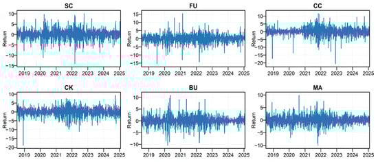
Figure 2.
Returns of China’s major energy futures.
Table 1 shows the descriptive statistics of China’s energy futures. The results show that SC has the highest average return, while CK and MA have the lowest, displaying some degree of negative returns. Additionally, CC exhibits the highest volatility. All return series show negative skewness, indicating longer left tails and suggesting more pronounced downside risk. The kurtosis values are significantly greater than 3, reflecting a clear leptokurtic distribution with fat tails. Furthermore, the Jarque–Bera (JB) statistics and Augmented Dickey–Fuller (ADF) unit root test results indicate that all return series significantly deviate from normality and are stationary within the sample period. Figure 3 displays the Pearson correlation coefficients among the six major energy futures. All return series exhibit positive correlations. Strong correlations are particularly evident between SC and FU, SC and BU, FU and BU, as well as CC and CK. SC, as the benchmark crude oil contract, significantly influences the price movements of downstream products like FU and BU. Meanwhile, CC and CK belong to the coal-coke industry chain, maintaining a close upstream–downstream relationship, which accounts for their high correlation.

Table 1.
Descriptive statistics of energy futures.
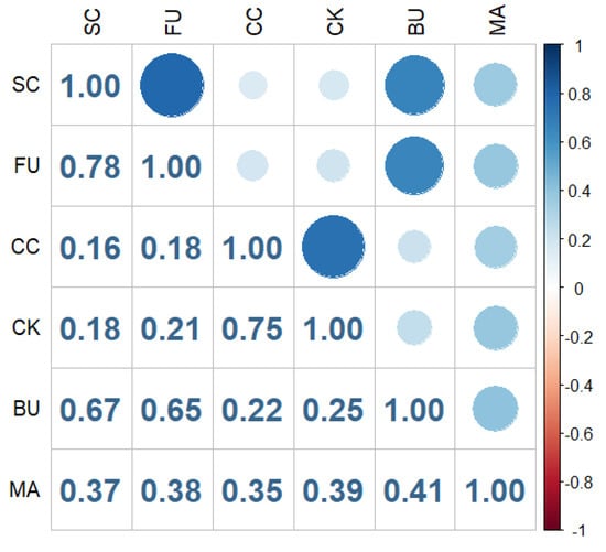
Figure 3.
Pearson correlation of energy futures.
In addition, this study employs a regression framework to examine the impact of weather variability on the risk spillovers of China’s energy futures, using temperature (TE), cooling degree days (CDD), heating degree days (HDD), and total precipitation (TP) as the core meteorological indicators. The weather data are obtained from the International Energy Agency’s (IEA) Weather, Climate and Energy Tracker, which is constructed based on ERA5 reanalysis and provides nationwide, daily frequency weather measures. It offers distinct advantages over the China Meteorological Agency’s local datasets, such as consistent spatial-temporal coverage and accessibility in conducting national-scale analysis. Accordingly, all weather variables used in this study represent the national averages for mainland China, enabling a consistent characterization of how overall climate conditions influence energy demand and the associated price dynamics. It is worth noting that existing studies have also employed such nationally aggregated weather data when examining the climate-energy nexus [29,47]. CDD and HDD are widely used demand-side indicators that capture temperature deviations driving cooling and heating needs accurately [55]. The thresholds of 26 °C (CDD) and 18 °C (HDD) are commonly adopted in Chinese energy studies because they align closely with observed patterns of cooling and heating energy use [56,57]. The control variables include geopolitical risk (GPR), CBOE volatility index (VIX), CBOE crude oil volatility index (OVX), and the CSI 300 Index (CSI300). The specific definitions of the weather variables are as follows:
- Temperature (TE): This indicator is the temperature of air at 2 m above the surface of land, sea or inland waters. It is calculated by interpolating between the lowest model level and the earth’s surface, taking account of the atmospheric conditions.
- Cooling Degree Days (CDD): This indicator reflects the extent to which the temperature exceeds the cooling base temperature (26 °C). It is calculated using the following expression: , where is the cooling degree days on day , and is the daily average temperature on that day.
- Heating Degree Days (HDD): This indicator reflects the extent to which the temperature falls below the heating base temperature (18 °C). It is calculated using the following expression: , where is the heating degree days on day , and is the daily average temperature on that day.
- Total Precipitation (TP): This indicator is the accumulated liquid and frozen water, comprising the rain and snow that falls to the earth’s surface. It is the sum of large-scale precipitation and convective precipitation.
4. Empirical Analysis
4.1. Static Spillover Results
This section applies the QVAR model to investigate spillover effects of China’s energy futures. To strengthen the explanatory power and comparability of the results, this paper uses OLS to estimate the spillover effects under the conditional mean as the benchmark of the traditional analytical framework. Subsequently, in order to reveal the heterogeneity of market spillovers under different conditions, the QVAR model is introduced to capture the spillover effects under normal, extreme downward and extreme upward market conditions at the 0.5, 0.05 and 0.95 quantiles, respectively. Table 2 presents the mean spillover results among China’s energy futures. The off-diagonal elements indicate the magnitude of spillover effects from one market to another. TSI measures the overall strength of spillover effects within the system. “TO” denotes the spillover effects transmitted from a specific market to others, while “FROM” indicates the spillover effect received from others. “NET” represents the net spillover effects, calculated as the difference between TO and FROM. A positive value implies the market is a net transmitter, whereas a negative value indicates it is a net recipient. In the QVAR model, the lag order is set to , based on the AIC Criterion, and the forecast step .
Table 2.
Static spillover results under conditional mean.
As shown in Table 2, the TSI under the conditional mean is 48.83%, indicating significant spillover effects among China’s energy futures markets. In terms of directional spillovers, the values of TO range from 33.86% to 59.5%, FROM ranges from 41.25% to 55.82%. Notably, SC is both the largest spillover transmitter and the primary spillover recipient, consistent with Gong et al. [58]. Markets with a high level of risk spillover are more likely to be impacted by other markets. Furthermore, MA exhibits the lowest spillover transmission and reception effects at 33.86% and 41.25%, respectively. Regarding net spillovers, CC and MA act as net recipients, with net spillovers of −1.93% and −7.38%, respectively, indicating they mainly absorb spillovers from other markets. In contrast, SC, FU, CK, and BU serve as net transmitters, with net spillover effects of 3.68%, 3.8%, 0.97%, and 0.86%, respectively. Among them, SC and FU are the primary sources of spillover transmission. Additionally, there is significant bidirectional mean spillover between CK and CC, as well as between FU and SC, similar to the findings of Wang et al. [49], which highlights the transmission effects between raw materials and finished energy products.
Table 3 presents the static spillover effects under normal market condition (0.5 quantile). Compared to the mean static spillovers, both exhibit similar spillover patterns [42]. For instance, FU and SC remain the largest risk spillover transmitters in the system. Furthermore, the roles of various energy futures in the system remain unchanged, while the spillover levels have undergone slight variation.
Table 3.
Static Spillover results at the 0.5 quantile.
Figure 4 displays the TSI under the conditional mean and across different quantile levels. The green dashed line represents the conditional mean, while the orange solid line shows the quantile-based results. It is evident that the TSI under extreme market conditions is consistently higher than under normal condition. This is because in extreme market conditions, especially during periods of extreme downturn, due to increased market panic and higher systemic risk exposure, the TSI significantly rises. Therefore, examining the spillover characteristics under extreme market conditions is of great importance for understanding the evolution of systemic risk [59].
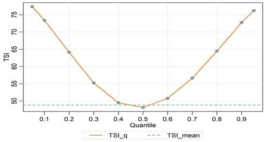
Figure 4.
Total spillover index (TSI): Conditional Mean vs. Quantiles (0.05–0.95).
Table 4 presents the spillovers among China’s energy futures under extreme downward (0.05 quantile) and extreme upward (0.95 quantile) market conditions. The TSI among China’s energy futures is 77.35% and 76.20%, respectively, under these two market conditions. Under extreme market conditions, the spillover effects from each energy future to itself decrease sharply compared to normal condition, while directional spillovers to other markets increase substantially. In terms of spillover effects among individual energy futures, spillover effects increase notably during extreme scenarios. Specifically, under extreme downward market condition, SC is the largest player in receiving and transmitting spillovers, accounting for 78.1% and 80.33%, respectively. Under extreme upward market condition, this role transforms into FU, with the spillovers it receives and transmits being 76.96% and 79.14%, respectively. Regarding the net spillover effects, SC, FU, CK, and BU act as net risk transmitters during extreme downside condition, with SC showing the highest net spillover of 2.22%. Under the extreme upward condition, SC, FU, and BU remain net transmitters, and FU becomes the most significant source of net spillover, at 2.18%. It is observed that under extreme conditions, CC exhibits the largest net negative spillover effects, reaching −2.26% and −4.17%, respectively. This indicates that under extreme conditions, CC can act as a stable spillover absorber in the system and be leveraged to hedge against severe risks of other assets.
Table 4.
Static spillover results at the 0.05 and 0.95 quantiles.
To further explain the extreme spillover patterns, CC acts as the largest net risk absorber at the 0.05 and 0.95 quantiles mainly because its demand is relatively stable and its price adjusts more slowly to shifts in market sentiment. Under extreme market conditions, this slower adjustment makes CC more likely to absorb spillovers transmitted from other energy products rather than amplify it. In contrast, FU and SC are positioned closer to the upstream side of the energy supply chain, where prices respond more quickly to changes in expectations, and broader market sentiment. As a result, they tend to react first during sharp market movements and transmit shocks outward.
Figure 5 presents the net paired spillover network structure of energy futures under different market conditions. In the figure, the color of the nodes indicates the role of each energy future within the system: red represents spillover transmitters, while yellow represents spillover recipients. The size of each node corresponds to the extent of its net spillover. The depth of color reflects the strength of pairwise spillovers (see the legend in Figure 5 for details), and the direction of the arrows indicates the direction of risk transmission. Overall, the spillover network shows significant structural differences under different scenarios, indicating the state dependence of the spillover effects. Under the conditional mean and 0.5 quantile, the network structure remains relatively stable, with SC and FU playing dominant roles in spillover transmission, while MA and CC act as spillover recipients, MA shows as the largest spillover recipient, presenting a strong characteristic of risk absorption. In extreme scenarios, the network structure undergoes significant structural changes. Specifically, in extreme conditions, the largest net risk recipient changes from MA to CC. The CC node shows more inward spillover connections and thicker edges, indicating that the spillover correlations between it and other energy futures are significantly enhanced, highlighting its spillover receiving role under extreme conditions. Meanwhile, SC becomes the most prominent spillover transmitter under extreme downward market condition, demonstrating its strong driving force for systemic spillovers. Additionally, CK demonstrates a clear role transformation depending on market conditions. In normal and extreme downward market conditions, it acts as a spillover transmitter. In upward market condition, its identity transforms into a spillover recipient.
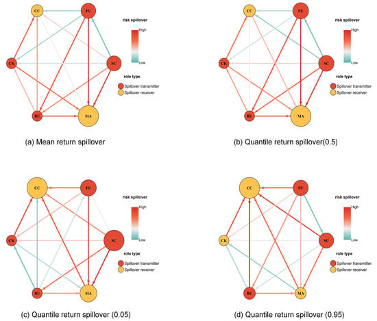
Figure 5.
Spillover networks.
4.2. Dynamic Spillover Results
Although static spillover analysis can observe the intensity and direction of spillover effects of China’s energy futures, it fails to explain the dynamic relationship of spillover effects. Therefore, this paper adopts the method combining the spillover index and the rolling window to explore the dynamic spillover relationship among China’s energy futures. This study employs a rolling window of 200 days.
Figure 6 shows the dynamic features of the TSI of China’s energy futures under the normal market condition and conditional mean. Overall, the trends of the two lines are largely consistent, both showing obvious characteristics of phased fluctuations over the entire observation period. Moreover, the evolution of TSI indicates that spillover effects of China’s energy futures market are significantly influenced by major external events. Specifically, in early 2020, the global outbreak of COVID-19 led to substantial fluctuations in oil prices and tightened market liquidity, leading to a sharp short-term rise in TSI. Subsequently, from 2021 to 2022, the TSI continued to rise and reached its peak in the middle of 2022. This stage coincides highly with the outbreak of the Russia-Ukraine conflict, the sharp fluctuations in international energy prices and the continuous tension in the global supply chain, reflecting the profound impact of global geopolitical conflicts on the energy market [60]. Since 2023, as the international energy market has gradually stabilized and domestic macroeconomic policy interventions have continued, the TSI has declined somewhat, suggesting a partial easing of spillovers. However, the TSI level remains at a historically high level, indicating that the risk transmission among markets is still in a strong state, and external uncertainties are still potentially affecting China’s energy futures market.
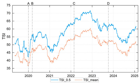
Figure 6.
Dynamic TSI based on the 0.5 quantile and conditional mean. Note: Event A: The outbreak of COVID-19. Event B: Fluctuations in international oil prices. Event C: The Russia-Ukraine conflict. Event D: The Hamas-Israel war.
To further depict the systemic spillover characteristics under different market conditions, this paper introduces TSI under extreme conditions and analyzes its dynamic evolution (see Figure 7). The results show that under extreme market conditions, the TSI level is significantly higher than that under normal market condition. Moreover, under extreme conditions, the TSI exhibits significant time-varying characteristics, reflecting the dynamic complexity of market spillover effects across the entire sample period. Compared to normal condition, the TSI fluctuates more sharply, indicating that spillover effects across markets are more intense when facing extreme scenarios like sudden market shocks or external crisis events. Further comparison reveals that the TSI under extreme downward market condition is significantly higher than that under extreme upward condition in most periods, reflecting the significant asymmetry of spillover effects of China’s energy futures market under extreme scenarios. Furthermore, the TSI under extreme market conditions also shows a strong response to major external events. During the global outbreak of the COVID-19 in 2020, the escalation of the Russia-Ukraine conflict in 2022, and the outbreak of the Hamas-Israel war in 2023, the TSI rises rapidly under extreme downward market condition, reflecting the sharp spread of spillovers driven by extremely negative events that disrupt global energy supply chains and market sentiment. In contrast, the TSI under extreme upside condition shows relatively moderate responses during the same periods, further confirming that the spillover effects of the energy futures market show significant asymmetry.
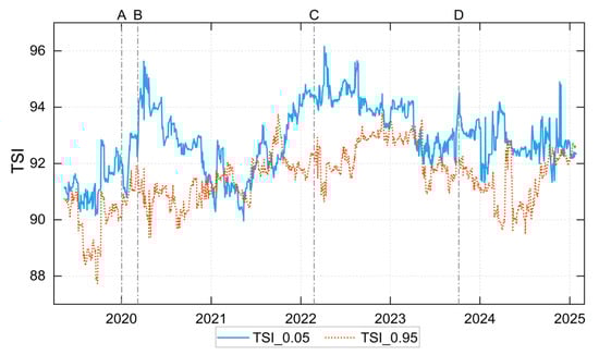
Figure 7.
Dynamic TSI based on the 0.05 and 0.95 quantiles. Note: The event annotations follow the same definitions as those shown in Figure 6.
4.3. The Impact of Weather Change on Spillover Effects of China’s Energy Futures
Table 5, Table 6 and Table 7 report the regression results analyzing how weather change factors affect the TSI in China’s energy futures under different market conditions, with each table corresponding to normal, extreme downward, and extreme upward states, respectively. The regression models incorporate key weather variables, including TE, CDD, HDD, TP, along with control variables such as GPR, OVX, VIX, Rate and CSI 300.
Table 5.
Regression results under normal market condition.
Table 6.
Regression results under extreme downward market condition.
Table 7.
Regression results under extreme upward market condition.
Table 5 shows the regression results under normal market condition. It shows that, among the weather variables, only CDD has a statistically significant effect on the TSI. Specifically, CDD exerts a positive impact on the TSI at the 1% significance level. This indicates that higher cooling demand induced by elevated temperatures increases overall energy consumption, which leads to more synchronized price movements across energy futures and thus stronger internal spillover transmission. TE, HDD, and TP are not statistically significant, implying that moderate temperature or precipitation fluctuations do not meaningfully alter supply–demand dynamics and therefore do not generate noticeable spillovers when the market is stable. For the control variables, GPR and VIX are significantly positive across all model specifications, indicating that heightened geopolitical or global uncertainty induces more homogeneous trading behavior and stronger co-movements among energy products, thereby amplifying spillovers. Conversely, Rate and CSI300 show significantly negative coefficients, suggesting that higher funding costs or stronger equity market performance reduce speculative activity in energy futures and disperse trading attention, which weakens co-movement and helps mitigate spillovers under normal conditions.
Table 6 presents the regression results under extreme downward market condition. Compared with the normal market condition, the explanatory power of the weather variables in the extreme downward situation is significantly enhanced. The model’s R2 value rises from approximately 0.20 to 0.36. This indicates that when the market drops sharply, the impact of weather change on the spillovers of the energy futures market is more significant. TE shows a significantly negative impact on the TSI in the extreme downward scenario, whereas it is insignificant under normal condition. This suggests that during periods of intense market panic, temperature fluctuations may ease short-term demand pressure or alter supply–demand expectations, thereby partially mitigating spillover transmission. CDD remains positive and highly significant across both market conditions; however, its coefficient is smaller under the extreme downside scenario. This implies that while high temperatures continue to amplify spillovers through increased cooling demand, their marginal effect may be dampened by panic-driven market behavior. Notably, HDD, which is insignificant under normal conditions, becomes significantly positive in the extreme downward market. This reflects that colder temperatures increase energy consumption and enhance market interconnectedness, thereby magnifying spillovers during severely negative conditions. Overall, these findings indicate that the market becomes more sensitive to weather-induced demand fluctuations during sharp downturns. Regarding the control variables, GPR, OVX, and VIX consistently show significantly positive coefficients, confirming that external uncertainty strengthens risk co-movement and spillovers during market stress. Rate and CSI300 remain significantly negative, suggesting that improved macroeconomic stability or stronger stock market performance helps ease risk spillovers even in extreme downward conditions.
Table 7 presents the regression results under the extreme upward market condition. Among the core explanatory variables, TE continues to exert a significant negative effect on the TSI, with a larger absolute coefficient. This suggests that the market becomes more sensitive to temperature fluctuations during strong upward trends. A plausible mechanism is that temperature changes alter expectations regarding production activity and supply capacity, and in a highly optimistic market, such expectation adjustments become more pronounced, thereby strengthening the mitigating effect of temperature on spillovers. In contrast to the normal and downward market conditions, CDD turns significantly negative under extreme upward conditions. This indicates that high temperatures do not amplify spillovers in a strongly rising market; instead, they may help suppress them. This pattern may arise because demand-driven effects associated with high temperatures have already been priced in during bullish conditions, and sentiment-driven trading dominates market behavior, diminishing or reversing the impact of CDD on spillovers. HDD remains significantly positive, reinforcing the notion that cold weather strengthens market interconnectedness by boosting energy consumption even during extreme upward movements. Additionally, TP shows a highly significant negative effect for the first time, implying that precipitation changes may alleviate supply pressure or reduce market synchronization, thereby helping curb systemic spillovers. GPR and VIX remain strongly positive, indicating that external uncertainty continues to amplify spillover effects in rising markets. However, OVX becomes significantly negative in this state, which is the opposite of its behavior under other market conditions. This result suggests that increased crude oil volatility may divert investor attention and reduce co-movements among energy futures during periods of strong bullish sentiment. Finally, Rate and CSI300 lose statistical significance, implying that when the market is dominated by optimism, the influence of macro-financial variables weakens substantially and becomes less relevant for explaining spillover behavior.
Overall, the effects of weather variables on the TSI differ clearly across the three market states. In normal markets, only CDD shows a significant positive impact, mainly because higher temperatures increase cooling demand and strengthen the joint demand movements of several energy products. In extreme downside markets, both CDD and HDD become strongly significant, indicating that when demand elasticity weakens and market sentiment turns pessimistic, increases in cooling or heating loads can intensify spillovers through a “demand contraction–price co-movement” mechanism. In extreme upside markets, by contrast, CDD and precipitation show stronger negative effects on spillovers, suggesting that under high demand expectations, weather changes trigger more differentiated supply–demand adjustments across products.
4.4. Robustness Check
To test the robustness of the research findings, we conduct a robustness test by replacing the original 0.05 and 0.95 quantiles with 0.1 and 0.9 quantiles to re-calculate the spillover index and verify the stability of the spillover effect characteristics across different extreme market condition definitions. Specific results of this quantile-replacement robustness test are shown in Appendix B (Table A2), and the findings confirm that the core characteristics of spillover effects. Meanwhile, this study initially constructs the spillover index using a baseline model with a 200-day rolling window and a 10-day forecast step. Based on this, we further re-estimate the spillover effects by adopting alternative settings, including rolling windows of 150 and 250 days and forecast steps of 5 and 15 days. Appendix B (Figure A1 and Figure A2) shows the dynamic evolution of the TSI under these different window lengths and forecast steps. The results show that, despite changes in the parameter settings, the overall dynamic patterns of the TSI remain consistent, demonstrating strong coherence and stability, thereby further confirming the robustness of the study’s conclusions. In addition, to verify the robustness of the regression analysis on the impact of weather change on systemic spillover effects, we replace the original core explanatory variables with the Yangtze River Delta Meteorological Index, which includes indices for temperature, cooling degree days, and heating degree days. Appendix C presents the regression results using these alternative variables. The findings indicate that although the core explanatory variables are altered, the main estimation results remain highly consistent with the previous regression models, providing support for the robustness of the conclusions of this paper.
5. Conclusions and Limitations
5.1. Conclusions
Based on the daily data of China’s six major energy futures from 16 July 2018, to 17 January 2025, this paper constructs a QVAR spillover framework to examine the risk spillover effects among energy futures under different market conditions. Furthermore, regression models are employed to investigate the impact of weather change on the spillover effects. The main findings are as follows:
Firstly, China’s energy futures market shows significant spillover heterogeneity under different market conditions. The total spillover index remains around 48% under normal market conditions but rises sharply to 77.35% and 76.20% in extreme downside and extreme upside markets, respectively. This indicates that during periods of extreme states, the transmission and linkage effects of spillovers among markets are more intense. Crude oil and fuel oil consistently serve as major spillover effect transmitters across various market states, while methanol and coking coal primarily act as spillover effect recipients. Notably, coking coal (−2.26% and−4.17%, respectively) demonstrates a stronger capacity to absorb spillovers under extreme conditions. To this end, we propose establishing a state-dependent risk monitoring and early warning system: integrate market state identification (normal/extreme upside/extreme downside) with systemic spillover intensity indicators, prioritize real-time tracking of risk transmission paths and key spillover transmitters, and strengthen targeted regulation in extreme market conditions.
Secondly, the spillover effects among China’s energy futures markets have significant time-varying characteristics. The rolling window analysis reveals that the total spillover index has experienced notable fluctuations during major external events such as the COVID-19 pandemic, the Russia–Ukraine conflict, and the Israel–Hamas war, indicating the market’s high sensitivity to external risks. Furthermore, under extreme market conditions, the total spillover index shows more intense volatility and asymmetry, highlighting the complexity of spillover transmission mechanisms in the energy market under extreme events. In this regard, it is essential to improve a flexible time-varying risk management framework: coordinate macroprudential tools and energy financial regulatory measures to dynamically adjust regulatory strategies in response to major external shocks (e.g., geopolitical conflicts, public health emergencies), thereby strengthening market resilience.
Finally, the impact of weather change on total spillover effects of the energy futures market exhibits significant state dependence. Under normal market condition, only the cooling degree days index shows a significant positive effect. In extreme downward market, temperature exerts a significant negative effect, while both heating degree days and cooling degree days significantly increase systemic spillovers. In extreme upward market, the negative effect of temperature intensifies, the effect of cooling degree days shifts from positive to negative, and precipitation acts as a significant factor suppressing spillover effects. These findings indicate that weather change affects market stability not only by altering supply and demand expectations but also by influencing risk transmission structures through differentiated mechanisms under different market conditions. Accordingly, policy efforts should focus on incorporating climate physical risk into energy financial governance: embed core meteorological indicators into energy derivatives pricing and risk assessment models, and promote the development of climate risk-oriented financial instruments to enhance market participants’ hedging capabilities against extreme weather events. Market participants, such as hedging operators and institutional investors, can use weather forecasts and climate indicators to adjust their strategies, optimizing hedging or investment decisions in response to weather-related risks.
To further clarify the spillover structure identified in this study, SC and FU consistently act as major spillover transmitters because they occupy core upstream positions in China’s energy value chains. SC serves as the primary pricing benchmark for refined oil and a wide range of petrochemical products, while FU is closely linked to refining margins and transportation costs. Their strong exposure to macroeconomic shocks and high information sensitivity enables their price fluctuations to spread rapidly to downstream markets. In contrast, CC and MA are subject to more rigid supply–demand constraints, causing them to function mainly as spillover receivers—especially under extreme market conditions, where their “shock-absorbing” role becomes more pronounced. The state-dependent effects of weather variables can also be explained through supply–demand elasticity. Under normal and downside market conditions, CDD significantly increases energy demand. This enhances interconnectedness across energy futures. However, during extreme upside markets, prices are dominated by speculative sentiment and expectation-driven dynamics. It weakens the marginal influence of cooling demand; consequently, CDD tends to dampen spillovers in such conditions. In contrast, HDD persistently increases heating demand and tightens supply conditions, thereby strengthening spillovers across all market states.
5.2. Limitations
Despite the insights provided, this study has several limitations. First, the weather variables are national averages, which may mask regional heterogeneity in energy demand responses; future studies could incorporate regional or city-level meteorological data. Second, as China’s energy system increasingly integrates renewable energy, future research could extend this framework to carbon futures, green electricity markets, and renewable-energy futures to better capture the interactions between climate risks and the evolving energy-financial system. In particular, integrating renewable energy futures and carbon derivatives into the same framework would help identify cross-market risk transmission channels between traditional energy markets and low-carbon financial instruments. Finally, this study has not yet conducted a mechanism analysis of the impact of weather change on energy futures spillover effects, and future research could supplement the exploration of this dimension with suitable micro-level data.
Author Contributions
Conceptualization, L.M.; methodology, L.M.; data curation, L.M.; software, L.M.; writing—original draft preparation, L.M.; writing—review and editing, G.C. and L.Z.; supervision, G.C. and L.Z.; project administration, G.C.; funding acquisition, G.C. All authors have read and agreed to the published version of the manuscript.
Funding
This research was funded by the Major Project of Philosophy and Social Science Research in Colleges and Universities of Jiangsu Province (Grant number 2022SJZD018); The China Meteorological Administration Climate Change Special Program (Grant number QBZ202402); The National Social Science Fund of China (Grant number 24BGL064).
Institutional Review Board Statement
Not applicable.
Informed Consent Statement
Not applicable.
Data Availability Statement
All data used in this study are available from the corresponding author upon reasonable request.
Conflicts of Interest
The authors declare no conflicts of interest.
Appendix A
Table A1.
Comparison of Applicability Among QVAR, TVP-VAR, and GARCH Models.
Table A1.
Comparison of Applicability Among QVAR, TVP-VAR, and GARCH Models.
| Model | Extreme-Risk Capture | Time-Varying Effect | Direction Identification | Computational Complexity | Energy-Futures Applicability |
|---|---|---|---|---|---|
| GARCH-based spillover | Weak (no tail dependence) | Weak (needs rolling windows) | Cannot (needs extensions) | Low–medium | Moderate (misses tail spillovers) |
| TVP-VAR spillover | Moderate | Strong (handles time-varying) | Can identify direction | High | Good (may smooth extremes) |
| QVAR spillover | Strong (tail/quantile) | Strong (state-dependent) | Clear (across quantiles) | Medium–high | Very high (normal/extreme markets) |
Appendix B
Table A2.
Static spillover results at the 0.1 and 0.9 quantiles.
Table A2.
Static spillover results at the 0.1 and 0.9 quantiles.
| SC | FU | CC | CK | BU | MA | FROM | |
|---|---|---|---|---|---|---|---|
| 0.1 quantile | |||||||
| SC | 25.19 | 20.16 | 10.88 | 11.73 | 18.29 | 13.75 | 74.81 |
| FU | 20.19 | 25.25 | 11.11 | 11.9 | 18 | 13.55 | 74.75 |
| CC | 11.83 | 11.98 | 28.84 | 20.71 | 12.44 | 14.21 | 71.16 |
| CK | 12.29 | 12.51 | 19.98 | 27.48 | 12.74 | 14.99 | 72.52 |
| BU | 18.31 | 17.94 | 11.65 | 12.22 | 25.71 | 14.16 | 74.29 |
| MA | 14.75 | 14.6 | 13.54 | 15 | 14.84 | 27.28 | 72.72 |
| TO | 77.37 | 77.2 | 67.16 | 71.55 | 76.31 | 70.67 | TSI |
| NET | 2.56 | 2.45 | −4.01 | −0.97 | 2.02 | −2.06 | 73.38 |
| 0.9 quantile | |||||||
| SC | 26.06 | 20.59 | 10.19 | 11.22 | 18.56 | 13.36 | 73.94 |
| FU | 20.6 | 26.09 | 10.31 | 11.63 | 17.91 | 13.46 | 73.91 |
| CC | 11.13 | 11.18 | 29.57 | 21.37 | 12.4 | 14.35 | 70.43 |
| CK | 11.72 | 12.14 | 20.34 | 27.98 | 12.7 | 15.11 | 72.02 |
| BU | 18.7 | 18.23 | 11.13 | 12.17 | 25.85 | 13.93 | 74.15 |
| MA | 14.31 | 14.2 | 13.7 | 15.01 | 14.8 | 27.97 | 72.03 |
| TO | 76.47 | 76.35 | 65.67 | 71.4 | 76.38 | 70.21 | TSI |
| NET | 2.54 | 2.44 | −4.76 | −0.62 | 2.22 | −1.82 | 72.75 |

Figure A1.
Dynamic spillover index under different rolling window sizes. Note: (a) shows the dynamic TSI under the0.5 quantile and conditional mean a with a 150-day rolling window; (b) shows the dynamic TSI under the 0.05 and 0.95 quantiles with a 150-day rolling window; (c) shows the dynamic TSI under the 0.5 quantile and conditional mean with a 250-day rolling window; (d) shows the dynamic TSI under the 0.05 and 0.95 quantiles with a 250-day rolling window.

Figure A2.
Dynamic spillover index under different forecast steps. Note: (a) shows the dynamic TSI under the 0.5 quantile and conditional mean with a 5-day forecast step; (b) shows the dynamic TSI under the 0.05 and 0.95 quantiles with a 5-day forecast step; (c) shows the dynamic TSI under the 0.5 quantile and conditional mean with a 15-day forecast step; (d) shows the dynamic TSI under the 0.05 and 0.95 quantiles with a 15-day forecast step.
Appendix C
Table A3.
Regression results under normal market condition.
Table A3.
Regression results under normal market condition.
| 1 | 2 | 3 | |
|---|---|---|---|
| TE | 0.0003 (1.005) | ||
| CDD | 0.0031 ** (3.006) | ||
| HDD | 0.0006 (0.668) | ||
| GPR | 0.0772 *** (10.583) | 0.0795 *** (10.885) | 0.0762 *** (10.505) |
| VOX | 0.0037 (0.221) | 0.0120 (0.721) | 0.0022 (0.133) |
| VIX | 0.1041 *** (6.157) | 0.0994 *** (5.886) | 0.1064 *** (6.333) |
| Rate | −0.4718 *** (−3.602) | −0.4578 *** (−3.511) | −0.4557 *** (−3.466) |
| CSI300 | −0.2389 *** (−5.034) | −0.2291 *** (−4.829) | −0.2391 *** (−5.036) |
| Constant | 6.2547 *** (9.711) | 6.1182 *** (9.502) | 6.2338 *** (9.653) |
| R-squared | 0.1106 | 0.1103 | 0.1106 |
Note: Values in parentheses are t-statistics. **, and *** indicate statistical significance at the 5%, and 1% levels, respectively.
Table A4.
Regression results under extreme downward market condition.
Table A4.
Regression results under extreme downward market condition.
| 1 | 2 | 3 | |
|---|---|---|---|
| TE | −0.00005 (−1.616) | ||
| CDD | 0.0003 *** (2.648) | ||
| HDD | 0.0002 ** (2.542) | ||
| GPR | 0.0054 *** (7.988) | 0.0058 *** (8.522) | 0.0055 *** (8.138) |
| OVX | 0.0074 *** (4.484) | 0.0086 *** (5.535) | 0.0080 *** (5.221) |
| VIX | 0.0144 *** (9.197) | 0.0136 *** (8.658) | 0.0143 *** (9.154) |
| Rate | −0.0552 *** (−4.532) | −0.0557 *** (−4.592) | 0.0531 *** (−4.358) |
| CSI300 | −0.0335 *** (−7.598) | −0.0324 *** (−7.330) | −0.0328 *** (−7.454) |
| Constant | 4.8208 *** (80.574) | 4.8073 *** (80.259) | 4.8083 *** (80.284) |
| R-squared | 0.3604 | 0.3625 | 0.3623 |
Note: Values in parentheses are t-statistics. **, and *** indicate statistical significance at the 5%, and 1% levels, respectively.
Table A5.
Regression results under extreme upward market condition.
Table A5.
Regression results under extreme upward market condition.
| 1 | 2 | 3 | |
|---|---|---|---|
| TE | −0.0002 *** (−6.868) | ||
| CDD | −0.0005 *** (−5.059) | ||
| HDD | 0.0004 *** (4.802) | ||
| GPR | 0.0053 *** (7.576) | 0.0054 *** (7.538) | 0.0058 *** (8.147) |
| OVX | −0.0049 *** (−3.068) | −0.0054 *** (7.538) | −0.0058 * (−1.961) |
| VIX | 0.0099 *** (6.050) | 0.0098 *** (5.861) | 0.0088 *** (5.373) |
| Rate | −0.0156 (−1.234) | −0.0215 (−1.691) | −0.0143 (−1.116) |
| CSI300 | 0.0043 (0.948) | 0.0035 (0.748) | 0.0062 (1.343) |
| Constant | 4.4474 *** (72.093) | 4.4949 *** (71.608) | 4.4492 *** (70.834) |
| R-squared | 0.1313 | 0.1175 | 0.1159 |
Note: Values in parentheses are t-statistics. *, and *** indicate statistical significance at the 10%, and 1% levels, respectively.
References
- Mao, X.; Wei, P.; Ren, X. Climate Risk and Financial Systems: A Nonlinear Network Connectedness Analysis. J. Environ. Manag. 2023, 340, 117878. [Google Scholar] [CrossRef] [PubMed]
- van Benthem, A.A.; Crooks, E.; Giglio, S.; Schwob, E.; Stroebel, J. The Effect of Climate Risks on the Interactions between Financial Markets and Energy Companies. Nat. Energy 2022, 7, 690–697. [Google Scholar] [CrossRef]
- Zhong, J.; Zhao, Y.; Li, Y.; Yan, M.; Peng, Y.; Cai, Y.; Cao, Y. Synergistic Operation Framework for the Energy Hub Merging Stochastic Distributionally Robust Chance-Constrained Optimization and Stackelberg Game. IEEE Trans. on Smart Grid 2025, 16, 1037–1050. [Google Scholar] [CrossRef]
- Zhou, S.; Yuan, D.; Zhang, F. Multiscale Systemic Risk Spillovers in Chinese Energy Market: Evidence from a Tail-Event Driven Network Analysis. Energy Econ. 2025, 142, 108151. [Google Scholar] [CrossRef]
- Zhao, G.; Yu, B.; An, R.; Wu, Y.; Zhao, Z. Energy System Transformations and Carbon Emission Mitigation for China to Achieve Global 2 °C Climate Target. J. Environ. Manag. 2021, 292, 112721. [Google Scholar] [CrossRef]
- Chen, Y.; Zhu, M.; Chen, M. Comprehensive Experimental Research on Wrapping Materials Influences on the Thermal Runaway of Lithium-Ion Batteries. Emerg. Manag. Sci. Technol. 2025, 5, e007. [Google Scholar] [CrossRef]
- Zhang, J.; Long, T.; Sun, X.; He, L.; Yang, J.; Wang, J.; Wang, Z.; Huang, Y.; Zhang, L.; Zhang, Y. Mechanism Investigation on Microstructure Degradation and Thermal Runaway Propagation of Batteries Undergoing High-Rate Cycling Process. J. Energy Chem. 2026, 113, 1013–1029. [Google Scholar] [CrossRef]
- Wang, L.; Ahmad, F.; Luo, G.; Umar, M.; Kirikkaleli, D. Portfolio Optimization of Financial Commodities with Energy Futures. Ann. Oper. Res. 2022, 313, 401–439. [Google Scholar] [CrossRef]
- Ren, Y.; Wang, N.; Zhu, H. Dynamic Connectedness of Climate Risks, Oil Shocks, and China’s Energy Futures Market: Time-Frequency Evidence from Quantile-on-Quantile Regression. N. Am. J. Econ. Financ. 2025, 75, 102263. [Google Scholar] [CrossRef]
- Shao, M.; Hua, Y. Price Discovery Efficiency of China’s Crude Oil Futures: Evidence from the Shanghai Crude Oil Futures Market. Energy Econ. 2022, 112, 106172. [Google Scholar] [CrossRef]
- Wang, J.; Qiu, S.; Yick, H.Y. The Influence of the Shanghai Crude Oil Futures on the Global and Domestic Oil Markets. Energy 2022, 245, 123271. [Google Scholar] [CrossRef]
- Dai, X.; Xiao, L.; Li, M.C.; Wang, Q. Toward Energy Finance Market Transition: Does China’s Oil Futures Shake up Global Spots Market? Front. Eng. Manag. 2022, 9, 409–424. [Google Scholar] [CrossRef]
- Chiaramonte, L.; Mecchia, F.; Paltrinieri, A.; Sclip, A. Geopolitical Risk and Energy Markets: Past, Present, and Future. J. Econ. Surv. 2025, 39, 2233–2253. [Google Scholar] [CrossRef]
- Baumeister, C.; Korobilis, D.; Lee, T.K. Energy Markets and Global Economic Conditions. Rev. Econ. Stat. 2022, 104, 828–844. [Google Scholar] [CrossRef]
- Liu, F.; Shao, S.; Li, X.; Pan, N.; Qi, Y. Economic Policy Uncertainty, Jump Dynamics, and Oil Price Volatility. Energy Econ. 2023, 120, 106635. [Google Scholar] [CrossRef]
- Wang, Q.; Li, R. Cheaper Oil: A Turning Point in Paris Climate Talk? Renew. Sustain. Energy Rev. 2015, 52, 1186–1192. [Google Scholar] [CrossRef]
- Fahmy, H. The Rise in Investors’ Awareness of Climate Risks after the Paris Agreement and the Clean Energy-Oil-Technology Prices Nexus. Energy Econ. 2022, 106, 105738. [Google Scholar] [CrossRef]
- Curcio, D.; Gianfrancesco, I.; Vioto, D. Climate Change and Financial Systemic Risk: Evidence from US Banks and Insurers. J. Financ. Stab. 2023, 66, 101132. [Google Scholar] [CrossRef]
- Ginglinger, E.; Moreau, Q. Climate Risk and Capital Structure. Manag. Sci. 2023, 69, 7492–7516. [Google Scholar] [CrossRef]
- Bressan, G.; Đuranović, A.; Monasterolo, I.; Battiston, S. Asset-Level Assessment of Climate Physical Risk Matters for Adaptation Finance. Nat. Commun. 2024, 15, 5371. [Google Scholar] [CrossRef]
- Steinberg, D.C.; Mignone, B.K.; Macknick, J.; Sun, Y.; Eurek, K.; Badger, A.; Livneh, B.; Averyt, K. Decomposing Supply-Side and Demand-Side Impacts of Climate Change on the US Electricity System through 2050. Clim. Change 2020, 158, 125–139. [Google Scholar] [CrossRef]
- Wen, F.; Chen, M.; Zhang, Y.; Miao, X. Oil Price Uncertainty and Audit Fees: Evidence from the Energy Industry. Energy Econ. 2023, 125, 106852. [Google Scholar] [CrossRef]
- Fant, C.; Boehlert, B.; Strzepek, K.; Larsen, P.; White, A.; Gulati, S.; Li, Y.; Martinich, J. Climate Change Impacts and Costs to U.S. Electricity Transmission and Distribution Infrastructure. Energy 2020, 195, 116899. [Google Scholar] [CrossRef] [PubMed]
- Loureiro, M.L.; Alló, M. Sensing Climate Change and Energy Issues: Sentiment and Emotion Analysis with Social Media in the U.K. and Spain. Energy Policy 2020, 143, 111490. [Google Scholar] [CrossRef]
- Chen, R.; Wei, B.; Jin, C.; Liu, J. Returns and Volatilities of Energy Futures Markets: Roles of Speculative and Hedging Sentiments. Int. Rev. Financ. Anal. 2021, 76, 101748. [Google Scholar] [CrossRef]
- Zhang, L.; Liang, C.; Huynh, L.D.T.; Wang, L.; Damette, O. Measuring the Impact of Climate Risk on Renewable Energy Stock Volatility: A Case Study of G20 Economies. J. Econ. Behav. Organ. 2024, 223, 168–184. [Google Scholar] [CrossRef]
- Hu, L.; Song, M.; Wen, F.; Zhang, Y.; Zhao, Y. The Impact of Climate Attention on Risk Spillover Effect in Energy Futures Markets. Energy Econ. 2025, 141, 108044. [Google Scholar] [CrossRef]
- Zhou, D.; Siddik, A.B.; Guo, L.; Li, H. Dynamic Relationship among Climate Policy Uncertainty, Oil Price and Renewable Energy Consumption—Findings from TVP-SV-VAR Approach. Renew. Energy 2023, 204, 722–732. [Google Scholar] [CrossRef]
- Xue, J.; Dai, X.; Zhang, D.; Nghiem, X.-H.; Wang, Q. Tail Risk Spillover Network among Green Bond, Energy and Agricultural Markets under Extreme Weather Scenarios. Int. Rev. Econ. Financ. 2024, 96, 103707. [Google Scholar] [CrossRef]
- Seok, S.; Cho, H.; Ryu, D. Intraday Analyses on Weather-Induced Sentiment and Stock Market Behavior. Q. Rev. Econ. Financ. 2024, 98, 101929. [Google Scholar] [CrossRef]
- Mosquera-López, S.; Uribe, J.M.; Joaqui-Barandica, O. Weather Conditions, Climate Change, and the Price of Electricity. Energy Econ. 2024, 137, 107789. [Google Scholar] [CrossRef]
- Man, Y.; Zhang, S.; He, Y. Dynamic Risk Spillover and Hedging Efficacy of China’s Carbon-Energy-Finance Markets: Economic Policy Uncertainty and Investor Sentiment Non-Linear Causal Effects. Int. Rev. Econ. Financ. 2024, 93, 1397–1416. [Google Scholar] [CrossRef]
- Li, J.; Liu, R.; Yao, Y.; Xie, Q. Time-Frequency Volatility Spillovers across the International Crude Oil Market and Chinese Major Energy Futures Markets: Evidence from COVID-19. Resour. Policy 2022, 77, 102646. [Google Scholar] [CrossRef]
- Jiang, W.; Zhang, Y.; Wang, K.-H. Analyzing the Connectedness among Geopolitical Risk, Traditional Energy and Carbon Markets. Energy 2024, 298, 131411. [Google Scholar] [CrossRef]
- Ben Salem, L.; Zayati, M.; Nouira, R.; Rault, C. Volatility Spillover between Oil Prices and Main Exchange Rates: Evidence from a DCC-GARCH-Connectedness Approach. Resour. Policy 2024, 91, 104880. [Google Scholar] [CrossRef]
- Diebold, F.X.; Yılmaz, K. On the Network Topology of Variance Decompositions: Measuring the Connectedness of Financial Firms. J. Econom 2014, 182, 119–134. [Google Scholar] [CrossRef]
- Baruník, J.; Křehlík, T. Measuring the Frequency Dynamics of Financial Connectedness and Systemic Risk. J. Financ. Econ. 2018, 128, 181–208. [Google Scholar] [CrossRef]
- Balcilar, M.; Gabauer, D.; Umar, Z. Crude Oil Futures Contracts and Commodity Markets: New Evidence from a TVP-VAR Extended Joint Connectedness Approach. Resour. Policy 2021, 73, 102219. [Google Scholar] [CrossRef]
- Antonakakis, N.; Chatziantoniou, I.; Gabauer, D. Refined Measures of Dynamic Connectedness Based on Time-Varying Parameter Vector Autoregressions. J. Risk Financ. Manag. 2020, 13, 84. [Google Scholar] [CrossRef]
- Ando, T.; Greenwood-Nimmo, M.; Shin, Y. Quantile Connectedness: Modeling Tail Behavior in the Topology of Financial Networks. Manag. Sci. 2022, 68, 2401–2431. [Google Scholar] [CrossRef]
- Bulut, E.; Marangoz, C. Exploring the Impact of Economic Recession Indicators on Global Financial Markets: A QVAR Analysis. Int. Rev. Financ. Anal. 2025, 99, 103966. [Google Scholar] [CrossRef]
- Jiang, D.; Jia, F.; Han, X. Quantile Return and Volatility Spillovers and Drivers among Energy, Electricity, and Cryptocurrency Markets. Energy Econ. 2025, 144, 108307. [Google Scholar] [CrossRef]
- Shao, S.F.; Cheng, J. Quantile Connectedness between Clean Energy Metals and China’s New Energy Market Segments. Appl. Econ. Lett. 2025, 1, 1–6. [Google Scholar] [CrossRef]
- Wei, Y.; Zhang, J.; Bai, L.; Wang, Y. Connectedness among El Niño-Southern Oscillation, Carbon Emission Allowance, Crude Oil and Renewable Energy Stock Markets: Time- and Frequency-Domain Evidence Based on TVP-VAR Model. Renew. Energy 2023, 202, 289–309. [Google Scholar] [CrossRef]
- Liu, W.; Tang, M.; Zhao, P. The Effects of Attention to Climate Change on Carbon, Fossil Energy and Clean Energy Markets: Based on Causal Network Learning Algorithms. Energy Strat. Rev. 2025, 59, 101717. [Google Scholar] [CrossRef]
- Lucidi, F.S.; Pisa, M.M.; Tancioni, M. The Effects of Temperature Shocks on Energy Prices and Inflation in the Euro Area. Eur. Econ. Rev. 2024, 166, 104771. [Google Scholar] [CrossRef]
- Zhao, Y.; Dai, X.; Zhang, D.; Wang, Q.; Cao, Y. Do Weather Conditions Drive China’s Carbon-Coal-Electricity Markets Systemic Risk? A Multi-Timescale Analysis. Financ. Res. Lett. 2023, 51, 103432. [Google Scholar] [CrossRef]
- Gonçalves, A.C.R.; Costoya, X.; Nieto, R.; Liberato, M.L.R. Extreme Weather Events on Energy Systems: A Comprehensive Review on Impacts, Mitigation, and Adaptation Measures. Sustain. Energy Res. 2024, 11, 4. [Google Scholar] [CrossRef]
- Wang, X.; Rong, X.; Yin, L. Discerning the Impact of Global Geopolitical Risks on China’s Energy Futures Market Spillovers: Evidence from Higher-Order Moments. Energy Econ. 2024, 140, 107981. [Google Scholar] [CrossRef]
- Almeida, D.; Ferreira, P.; Dionísio, A.; Aslam, F. Exploring the Connection between Geopolitical Risks and Energy Markets. Energy Econ. 2024, 141, 108113. [Google Scholar] [CrossRef]
- Gu, Q.; Li, S.; Tian, S.; Wang, Y. Climate, Geopolitical, and Energy Market Risk Interconnectedness: Evidence from a New Climate Risk Index. Financ. Res. Lett. 2023, 58, 104392. [Google Scholar] [CrossRef]
- Hong, Y.; Luo, K.; Xing, X.; Wang, L.; Huynh, L.D.T. Exchange Rate Movements and the Energy Transition. Energy Econ. 2024, 136, 107701. [Google Scholar] [CrossRef]
- Zhang, H.; Chen, J.; Shao, L. Dynamic Spillovers between Energy and Stock Markets and Their Implications in the Context of COVID-19. Int. Rev. Financ. Anal. 2021, 77, 101828. [Google Scholar] [CrossRef] [PubMed]
- Chen, Y.; Zhu, H.; Liu, Y. Measuring Multi-Scale Risk Contagion between Crude Oil, Clean Energy, and Stock Market: A MODWT-Vine-Copula Method. Res. Int. Bus. Financ. 2025, 75, 102790. [Google Scholar] [CrossRef]
- Shi, Y.; Zhang, D.F.; Xu, Y.; Zhou, B.-T. Changes of Heating and Cooling Degree Days over China in Response to Global Warming of 1.5 °C, 2 °C, 3 °C and 4 °C. Adv. Clim. Change Res. 2018, 9, 192–200. [Google Scholar] [CrossRef]
- Guo, Y.Y.; Teng, M.X.; Zhang, C.; Wang, S.N.; Wei, Y.M. Climatic Impacts on Electricity Consumption of Urban Residential Buildings in China. Adv. Clim. Change Res. 2025, 16, 25–34. [Google Scholar] [CrossRef]
- Shen, H.; Wen, X.; Trutnevyte, E. Accuracy Assessment of Energy Projections for China by Energy Information Administration and International Energy Agency. Energy Clim. Change 2023, 4, 100111. [Google Scholar] [CrossRef]
- Gong, X.L.; Zhao, M.; Wu, Z.C.; Jia, K.W.; Xiong, X. Research on Tail Risk Contagion in International Energy Markets—The Quantile Time-Frequency Volatility Spillover Perspective. Energy Econ. 2023, 121, 106678. [Google Scholar] [CrossRef]
- Le, T.H. Quantile Time-Frequency Connectedness between Cryptocurrency Volatility and Renewable Energy Volatility during the COVID-19 Pandemic and Ukraine-Russia Conflicts. Renew. Energy 2023, 202, 613–625. [Google Scholar] [CrossRef]
- Jin, Y.; Zhao, H.; Bu, L.; Zhang, D. Geopolitical Risk, Climate Risk and Energy Markets: A Dynamic Spillover Analysis. Int. Rev. Financ. Anal. 2023, 87, 102597. [Google Scholar] [CrossRef]
Disclaimer/Publisher’s Note: The statements, opinions and data contained in all publications are solely those of the individual author(s) and contributor(s) and not of MDPI and/or the editor(s). MDPI and/or the editor(s) disclaim responsibility for any injury to people or property resulting from any ideas, methods, instructions or products referred to in the content. |
© 2025 by the authors. Licensee MDPI, Basel, Switzerland. This article is an open access article distributed under the terms and conditions of the Creative Commons Attribution (CC BY) license.