Slow-Coherency-Based Controlled Splitting Strategy Considering Wind Power Uncertainty and Multi-Infeed HVDC Stability

Abstract

In the context of a high proportion of renewable energy integration, active splitting section search—one of the “three defense lines” of a power system—is crucial for the security, stability, and long-term sustainability of islanded grids. Addressing the random fluctuations of high-penetration wind power and the weakened voltage support capability caused by multi-infeed HVDC, this paper proposes a slow-coherency-based active splitting section optimization model that explicitly accounts for wind power uncertainty and multi-infeed DC stability constraints. First, a GMM-K-means method is applied to historical wind data to model, sample, and cluster scenarios, efficiently generating and reducing a representative set of typical wind outputs; this accurately captures wind uncertainty while lowering computational burden. Subsequently, an improved particle swarm optimizer enhanced by genetic operators is used to optimize a multi-dimensional coherency fitness function that incorporates a refined equivalent power index, frequency constraints, and connectivity requirements. Simulations on a modified New England 39-bus system demonstrate that the proposed model markedly enlarges the post-split voltage stability margin and effectively reduces power-flow shocks and power imbalance compared with existing methods. This research contributes to enhancing the sustainability and operational resilience of power systems under energy transition.

1. Introduction

In the context of the development of new-type power systems, the typical characteristics have become the high penetration of renewable energy, high proportion of DC infeed, and hybrid AC/DC grid architecture. While this structure enhances the clean energy utilization and inter-regional transmission capacity, it also brings challenges such as system inertia reduction, weakened voltage support, increased risk of cascading failures in multi-infeed DC systems, and a deep coupling between angle and voltage stability [1,2,3]. As a crucial defense line in the security and stability control system, Active Controlled Islanding technology comprehensively utilizes global information to dynamically generate reasonable separation boundaries. It decouples the disturbed system into multiple islands capable of synchronized and stable operation, providing a solution to contain accident spread and prevent large-scale blackouts. Within this technical framework, selecting the optimal islanding boundary remains the core research challenge. Academia has explored effective solutions focusing on Slow Coherency Theory and Graph Theory, achieving significant progress [4].

In the aspect of Graph Theory and intelligent algorithm solutions, scholars have also contributed abundant theoretical results. Given that the graph theory method is inherently an NP-complete problem, as proven in reference [5], creative algorithms such as Depth-First Search, Breadth-First Search, and Ordered Binary Decision Diagrams were introduced in reference [6,7,8] to search for the optimum within a vast solution space. Reference [9] proposed a linear programming-based probabilistic search algorithm that starts from a randomly selected initial point and aims to find the optimal boundary by minimizing the power imbalance. To effectively address the risk of system loss of synchronism, Mixed Integer Linear Programming (MILP) was used for modeling and solving in reference [10]. However, some models only target the minimization of load shedding, neglecting the coherency relationship among generator groups. Although coherency constraints were introduced in reference [11], a simplified DC power flow was used to handle island power balance, which neglected the effect of reactive power, thus affecting the accuracy of the results. The MILP islanding models in reference [12,13] primarily minimize the power imbalance as the optimization objective, failing to fully consider the transient instability risk caused by power-flow shocks. This may lead to hidden stability dangers in the resulting islanding schemes during actual operation.

Reference [14] successfully constructed a simplified system model with topological connectivity constraints and applied a Genetic Algorithm to solve for the boundary. Regarding the development and application of the Slow Coherency Theory, references [15,16] performed multi-scale analysis of system dynamic responses, first clarifying the application conditions and limitations of the theory. Based on the aggregation characteristics of slow modes, they proposed a coordinated optimization method for the islanding boundary and island operating area, significantly enhancing the unit coherency stability during island operation.

With the rapid development of new-type power systems characterized by high penetration of renewable energy and multi-infeed DC systems, existing methods face shortcomings in complex operating scenarios. Firstly, they insufficiently account for the uncertainty of high-penetration wind power output, potentially leading to designed islanding schemes that cannot adapt to the real-time fluctuations of wind power in actual operation, thus affecting the robustness of the islanding strategy. Secondly, traditional indicators like the Short Circuit Ratio (SCR) only consider multi-DC infeed, and the L-index only considers multi-load outfeed, failing to fully account for the comprehensive support capability of multi-infeed DC systems to the AC grid.

Therefore, to enhance the stability of the system after islanding, this paper proposes an active islanding boundary optimization model that considers the uncertainty of wind power generation and the stability of multi-infeed HVDC systems, and verifies the reliability of the model by achieving the following specific objectives: (1) To accurately model wind power uncertainty by proposing a Gaussian Mixture Model-K-means (GMM-K-means) method for scenario generation and reduction, enhancing the adaptability of islanding schemes to real-time fluctuations; (2) To improve post-splitting voltage stability in multi-infeed HVDC systems by introducing an Improved Equivalent Power Index (IEPI) into the optimization model; (3) To develop an effective solution algorithm by designing a genetic-inspired improved particle swarm optimization (GA-IPSO) algorithm capable of solving the resulting complex nonlinear optimization problem; (4) To validate the proposed framework through comprehensive simulations on a modified New England 39-bus system, demonstrating its superiority in enhancing voltage stability margin and reducing power-flow shocks compared to existing methods.

2. An Improved Model for Slow-Coherency Node Relevance

2.1. Basic Principles of Slow-Coherency Grouping

In the linearized power-system model, the slow electromechanical oscillation modes that mirror the “swing-together” tendency of generators are first extracted. Units are then clustered according to their participation in these slow modes: generators whose participation factors are alike are assigned to the same “slow-coherency group”. Even under large disturbances, machines inside one group tend to stay mutually synchronous, whereas the inter-group links are weak and can be chosen as splitting surfaces, thereby partitioning the large-scale grid into several dynamically quasi-independent sub-areas.

To enhance the accuracy of power-system coherency identification, this paper adopts the improved strategy proposed in reference [5] and replaces the traditional power angle with the generator terminal-voltage phase angle as the state variable. First, the generator rotor-motion equations are linearized around their equilibrium operating point; then the conventional eigenvalue problem is generalized to the generalized eigenvalue problem form:

$${\displaystyle \frac{d^2\mathsf{\Delta }\delta }{d{t}^2}}=M^{-1}K\mathsf{\Delta }\delta =A\mathsf{\Delta }\delta$$

(1)

$$(A - \lambda E)\mathit{v} =0$$

(2)

$$E=\left[\begin{array}{cc}{I}_{\mathrm{m}}& \mathrm{0}\\ \mathrm{0}& \mathrm{0}\end{array}\right] \in R^{(\mathrm{m}+\mathrm{n})\times (\mathrm{m}+\mathrm{n})}$$

(3)

$M = \mathrm{diag}\left[M_1,M_2,\dots {,M}_{\mathrm{m}}\right]$ denotes the generator inertia matrix; m and n are the numbers of generator and non-generator buses, respectively; $\mathsf{\Delta }\delta$ is the deviation of the generator power angle from its equilibrium value; K is the system state matrix; $A \in R^{(\mathrm{m}+\mathrm{n})\times (\mathrm{m}+\mathrm{n})}$ is the partial derivative of bus power with respect to bus phase angle; $I_{\mathrm{m}}$ is the m-dimensional identity matrix.

To effectively identify the dominant oscillation modes of the power system, we sort them by the absolute value of their damping time constants in ascending order and calculate the following indicators:

$$K = {\displaystyle \frac{\left|{\lambda }_r\right|}{\left|{\lambda }_{r+1}\right|}} = \underset{i=2,3,\dots ,\mathrm{m}-1}{\min }{\displaystyle \frac{\left|{\lambda }_i\right|}{\left|{\lambda }_{i+1}\right|}}$$

(4)

${\lambda }_1,{\lambda }_2,\dots ,{\lambda }_r$, the first r eigenvalues, are selected as the dominant modes, and the eigenvectors corresponding to these dominant modes form the modal space basis of the system. Subsequently, the r columns of eigenvectors associated with the dominant modes constitute the modal matrix $V_r$. By applying Gaussian elimination–based operations to this modal matrix, we ultimately obtain the relevance matrix S that characterizes the slow-coherency properties.

2.2. Node-Relevance Classification and System Coherency Analysis

In power-system slow-coherency analysis, the entries of the slow-coherency relevance matrix quantify how strongly each node is associated with a specific slow-coherency group. Building on this theory, reference [13] proposes a node classification criterion based on the relevance matrix that rigorously distinguishes the coherency characteristics of individual nodes:

(1)

$\Vert S_i\Vert > \theta$, $\theta$ is an extremely small positive number;

(2)

There exists a k, such that $A_{j,k } = {\displaystyle \frac{\left|S_{j,k }\right|}{\Vert S_r\Vert }} = \eta \to 1$, where $\Vert *\Vert$ denotes $\Vert S_i\Vert = \sqrt{{\lambda }_{\max }\left(S_i^{\mathrm{T}}{S}_i\right)}$

(3)

$d_i = \sqrt{{\displaystyle \frac{{\sum _{k=1}^r\left(A_{ik}-\max (A_{ik})\right)}^2}{r-1}} }> \sigma$, where σ is a positive number. The larger the value of σ, the stricter the requirements for a node to be classified as a mode node.

Based on the above multi-dimensional dynamic criteria, this paper refines the classification of power-system nodes as follows:

Mode nodes: nodes that simultaneously satisfy Criteria 1, 2, and 3. They are strongly and uniquely coupled to a specific slow-coherency group; in any splitting strategy they must be strictly assigned to the corresponding island.

Ambiguous nodes: nodes that satisfy Criterion 1 but fail Criterion 2 or 3. Under different disturbances they may exhibit relevance to different slow-coherency groups, so their regional affiliation is uncertain and can significantly increase the complexity of islanding decisions.

Weak-link nodes: nodes that do not satisfy Criterion 1. They can be used as flexible boundaries between islands.

The spatial distribution of node types directly governs the decision dimension of any splitting strategy. Mode nodes impose hard partition constraints, weak-link nodes provide flexible adjustment space, while ambiguous nodes may trigger a Boolean-satisfiability problem. When a large number of ambiguous nodes are scattered throughout the system, it signals the absence of a clear slow mode and makes the selection of a suitable splitting surface extremely difficult [13]. To address this, structural grid reinforcement that converts node types can reshape the decision space into an advantageous pattern of “globally dominant determinism plus locally controllable degrees of freedom”, effectively reducing the computational complexity of islanding and simultaneously enhancing transient-stability margins.

3. Wind Power Output Scenarios and DC Infeed Stability Criteria

3.1. Wind Power Scenario Generation and Reduction Based on GMM

3.1.1. Rationale for Method Selection

For modeling the uncertainty of wind power output, existing methods can be categorized into two major classes: probabilistic modeling and data-driven approaches, each with distinct characteristics and application scenarios. Probabilistic methods, such as Copula models, can flexibly capture the spatial dependency structure among multiple wind farms, but their ability to represent high-dimensional temporal correlations is limited, and they often involve high computational complexity in the scenario generation and reduction process [17]. Time-series forecasting methods, such as Long Short-Term Memory (LSTM) networks, excel at capturing the temporal characteristics of wind power output and are suitable for short-term forecasting. However, their outputs are typically deterministic values or probabilistic intervals, making it difficult to directly generate the “scenario sets” required for subsequent stochastic optimization. Moreover, these models rely on large datasets for training and incur high computational costs [18]. Generative models, such as Generative Adversarial Networks (GANs) and Variational Autoencoders (VAEs), can learn complex data distributions and generate high-quality scenarios. Nevertheless, these methods suffer from unstable training processes, are prone to mode collapse, and their generated results often lack interpretability and controllability, making them difficult to integrate directly into physics-constrained optimization models for power systems.

Given the need for computational efficiency, interpretability, and multimodal distribution modeling in power system optimization, this paper employs a GMM combined with K-means clustering. This hybrid approach is selected because it effectively captures the multimodal nature of wind power through multiple Gaussian components, allows efficient parameter estimation via the Expectation-Maximization algorithm, and enables fast scenario reduction to support real-time decision-making.

3.1.2. Principle of GMM

Conventional wind power scenario generation often relies on Monte Carlo (MC) sampling, which suffers from slow convergence and sampling bias with limited data [19]. To address this, we employ a GMM-based framework that approximates the empirical distribution as a weighted sum of Gaussian components. Unlike single-distribution methods, GMM naturally accommodates multimodality arising from distinct weather regimes. Parameters are adaptively learned via the EM algorithm, avoiding manual tuning and supporting multivariate extension for spatial-temporal correlation modeling. Coupled with K-means clustering for scenario reduction, the approach maintains statistical representativeness while lowering computational burden in subsequent optimization. The mathematical formulation is presented below:

$$p\left(x\right)={\sum }_{k=1}^K{\pi }_k\left(x\mid {\mu }_k,{\Sigma }_k\right)$$

(5)

K represents the total count of Gaussian mixture components; ${\pi }_k$ is the mixing coefficient of the k-th Gaussian component; μₖ and Σₖ are the respective mean vector and covariance matrix of the k-th Gaussian component. Figure 1 shows the probability distribution of wind power output under different wind speed conditions. The x-axis represents wind power output in megawatts (MW), and the y-axis represents probability density.

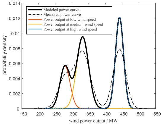
Figure 1. The principle of wind power output scenario generation based on GMM (source: simulation results of this study).

3.1.3. Implementation Steps of the GMM Method

(1)

Data preprocessing: collect historical wind power output data$\{x_1,{ x}_2,\dots ,x_{\mathrm{N}}\}$ and standardize it. For time-series data, sliding-window features can be extracted.

(2)

Estimate GMM parameters with the EM algorithm.

Initialization: randomly assign Gaussian means, covariances, and mixing weights.

E-step: compute the posterior probability of each sample belonging to every Gaussian component.

$${\pi }_k={\displaystyle \frac{1}{\mathrm{N}}}{\sum }_{n=1}^{\mathrm{N}}{\gamma }_{nk};{ \mu }_k={\displaystyle \frac{\sum _{n=1}^{\mathrm{N}}{\gamma }_{nk}{x}_n}{\sum _{n=1}^{\mathrm{N}}{\gamma }_{nk}}}$$

(6)

M-step: update the model parameters.

$${\Sigma }_k={\displaystyle \frac{\sum _{n=1}^{\mathrm{N}}{\gamma }_{nk}(x_n-{\mu }_k\left)\right(x_n-{\mu }_k{)}^{\mathrm{T}}}{\sum _{n=1}^{\mathrm{N}}{\gamma }_{nk}}}$$

(7)

${\gamma }_{nk}$ represents the posterior probability that the n-th sample belongs to the k-th Gaussian component. $x_n$ represents the observed value of the n-th sample. $\mathrm{N}$ represents the total number of samples. ${\Sigma }_k$ represents the covariance matrix of the k-th Gaussian component.

(3)

Scenario generation: randomly select a Gaussian component according to the mixing coefficient ${\pi }_k$, then sample from the chosen Gaussian distribution $\mathrm{N}\left(x|{\mu }_k,{\Sigma }_k\right)$.

(4)

Repeat the above steps N times until all sub-intervals are covered, finally obtaining an initial set $\{s_1, s_2,{ s}_3, ...,{ s}_{\mathrm{N}}\}$ that contains N raw wind power output scenarios.

(5)

Scenario reduction: to lower the computational complexity of wind power scenarios, this study employs a probability distance-based K-Means scenario reduction technique. Using The Silhouette Coefficient as the quality gauge, the method trims the original N scenarios down to S representative ones while guaranteeing that the reduced set faithfully preserves the distributional characteristics of the full data.

The reduced scenario set must satisfy the following optimization conditions:

$$\min {\sum }_{i=1}^S{\sum }_{j=1}^S‖W_s^{\left(i\right)}-W_s^{\left(j\right)}‖$$

(8)

In the equation: ||*|| represents the Euclidean distance formula; $W_s^{\left(i\right)}$ represents the wind power output.

The Silhouette Coefficient $s$ is used to evaluate the clustering quality, and its calculation formula is

$$s ={\displaystyle \frac{b-a}{\max (a,b)}}$$

(9)

Here, a is the average distance from a sample point to all other points within the same cluster, known as the intra-cluster distance. Meanwhile, b is the average distance from the sample point to all points in the nearest neighboring cluster, known as the inter-cluster distance.

Table 1 presents the three typical scenarios of the wind farm, which are derived from the actual output data of a 600 MW installed capacity wind farm. This study takes the original operational data of the wind farm as the input dataset and processes it using the proposed scenario reduction algorithm. Through iterative optimization and convergence analysis of the scenario set, redundant scenarios are eliminated, and the optimized scenario set ultimately converges to the three representative typical scenarios summarized in Table 1.

Table 1. Typical scenarios of the wind farm (source: simulation results of this study).

Scenario	Wind Farm Output/MW	Probability
1	279.11	21.2%
2	331.87	42.2%
3	442.15	36.6%

3.2. Improved Equivalent Power Index

Reference [20] simplifies the AC side into an ideal voltage source, ignoring both the voltage-dependent characteristic of loads and the Q–V response of renewable plants. To evaluate the voltage stability of AC/DC hybrid systems that contain wind farms more accurately, this paper adopts an improved multi-port Thévenin-equivalent approach. During the equivalence: conventional units and renewable generators with voltage-regulation capability are represented as voltage sources; ZIP loads and outgoing HVDC links are treated as current sources feeding out; Receiving-end HVDC links and PQ controlled renewable units that have hit their reactive power limits are regarded as current sources feeding in. The terms associated with the voltage-source set V and the current-source set I are then classified as follows:

$$U_i-{\sum }_{j\in V}{Z}_{ij}{I}_j ={ Z}_{ii}{\sum }_{j\in I}{\displaystyle \frac{Z_{ij}}{Z_{ii}}}{I}_j$$

(10)

Let the voltage-source terms on the left-hand side of the equation be denoted as $U_{ij}$, and the current-source terms on the right-hand side be denoted as $I_{\mathrm{e}\mathrm{q} }$:

$$U_{xi} = {\sum }_{j\in U}{Z}_{ij}{I}_j$$

(11)

$$I_{\mathrm{eq}}=-{\sum }_{j\in I}{\displaystyle \frac{Z_{ij}}{Z_{jj}}}{I}_j$$

(12)

$$S_{\mathrm{eq}}={\sum }_{j\in I}{\displaystyle \frac{Z_{ij}^{*}}{Z_{\mathrm{ii}}}}·{\displaystyle \frac{U_i}{U_j}}{S}_j$$

(13)

$Z_{ij}^{*}$ represents the complex conjugate of $Z_{ij}$, $Z_{ij }^{*}$ represents the complex conjugate of $Z_{\mathit{ii}}$, and $S_j$ denotes the complex power corresponding to node j. Based on the voltage-stability criterion, the voltage-stability factor is obtained as

$$K_{\mathit{VSF}}= \underset{\mathsf{\Delta }{Q}_i\to 0}{\lim }{\displaystyle \frac{\mathsf{\Delta }{Q}_i}{\mathsf{\Delta }{U}_i}}$$

(14)

At the critical point of static voltage instability:

$$K_{\mathit{VSF}} = \underset{\mathsf{\Delta }{Q}_i\to 0}{\lim }{\displaystyle \frac{\mathsf{\Delta }{Q}_i}{\mathsf{\Delta }{U}_i}} = 0$$

(15)

$${\mathit{VSF}}_i={\left[U_i\left(U_i^{\mathrm{T}}{Y}_{{\mathrm{eq}}_i}+Q_{{\mathrm{eq}}_i}\right)\right]}^{-1}\left[\begin{array}{c}{U}_i^{\mathrm{T}}{Y}_{{\mathrm{eq}}_i}^2-2Q_{{\mathrm{eq}}_i}{U}_i^{\mathrm{T}}{Y}_{{\mathrm{eq}}_i}+Q_{{\mathrm{eq}}_i}^2-S_{{\mathrm{eq}}_i}^2\\ +{ U}_i{\displaystyle \frac{\partial Q_{\mathrm{eq}}}{\partial U_i}}\left(U_i^{\mathrm{T}}{Y}_{{\mathrm{eq}}_i}+Q_{{\mathrm{eq}}_i}\right)+U_i{\displaystyle \frac{\partial P_{\mathrm{eq}}}{\partial U_i}}{P}_{{\mathrm{eq}}_i}\end{array}\right]$$

(16)

$$D_{{\mathit{EPI}}_i}=\sqrt{{\displaystyle \frac{U_i^{\mathrm{T}}{Y}_{{\mathrm{eq}}_i}^2+U_i\frac{\partial Q_{{\mathrm{eq}}_i}}{\partial U_i}{Q}_{{\mathrm{eq}}_i}+U_i\frac{\partial P_{{\mathrm{eq}}_i}}{\partial U_i}{P}_{{\mathrm{eq}}_i}}{S_{{\mathrm{eq}}_i}^2+U_i^3\frac{\partial Q_{{\mathrm{eq}}_i}}{\partial U_i}{Y}_{{\mathrm{eq}}_i}}}}$$

(17)

In Equation (17), $P_{{\mathrm{eq}}_i}$ represents the active power component $S_{{\mathrm{eq}}_i}$, $Q_{{\mathrm{eq}}_i}$ represents the reactive power component of $S_{{\mathrm{eq}}_i}$, and $Y_{{\mathrm{eq}}_i}$ represents the self-impedance of node i. The numerator represents the system’s capability to maintain voltage stability, while the denominator reflects the power demand stress imposed on the system. To account for the enhancing effect of dynamic reactive power support on static voltage stability, a dynamic correction factor is defined as

$$\eta =1 +\alpha {\displaystyle \frac{Q_{\mathrm{reserve}}}{Q_{\mathrm{load}}}}$$

(18)

where ${ Q}_{\mathrm{reserve}}$ is the total reactive power reserve near the critical node, ${ Q}_{\mathrm{load}}$ denotes the reactive power demand of the load, and α is the normalized sensitivity of the stability margin to the reactive power reserve.

$$K_{{\mathit{EPI}}_i}=\eta D_{{\mathit{EPI}}_i}$$

(19)

When the power system reaches its voltage-stability limit, there exists at least one node i for which $K_{\mathit{EPl}} = 1$. During stable operation, $K_{\mathit{EPI} }> 1$ at every node. If the system is unstable, there exists at least one node i with $K_{\mathit{EPI}} < 1$.

4. Solving the Mathematical Model for Active Splitting-Surface Search

4.1. Mathematical Model

4.1.1. Objective Function

In power-system dynamic-performance analysis, optimal reconfiguration of the network topology can markedly improve nodal slow-coherency characteristics. An ideal grid structure should simultaneously satisfy the following requirements: the fraction of mode nodes among all system buses is maximized; the fraction of mode nodes among non-weak-link buses is maximized; the average coherency relevance of mode nodes to their own slow-coherency group is maximized; the average coherency relevance of mode nodes to external slow-coherency groups is minimized. Accordingly, four complementary objective functions are formulated to quantify the optimization effectiveness:

(1)

Ratio of mode nodes to the total number of system buses:

$$f_a={\displaystyle \frac{{\sum }_{i=1}^k{N}_{mi}}{{\sum }_{i=1}^k{N}_{si}}}$$

(20)

(2)

Ratio of mode nodes to non-weak-link nodes:

$$f_b={\displaystyle \frac{\sum _{i=1}^k{N}_{mi}}{\sum _{i=1}^k(N_{mi}+N_{di})}}$$

(21)

(3)

Mean value of the correlation between a mode node and its coherency group:

$$f_c={\displaystyle \frac{\sum _{i=1}^k\sum _{c\in N_{mi}}{A}_{cc}}{\sum _{i=1}^k{N}_{mi}}}$$

(22)

(4)

Average relevance of mode nodes to external (non-own) slow-coherency groups:

$$f_d={\displaystyle \frac{\sum _{i =1}^k\sum _{c=1}^{{\mathrm{N}}_{mi }}\sum _{d=1}^r{A}_{cd}}{\left(r\times \sum _{i=1}^{k }{N}_{mi}\right)}}$$

(23)

In the above expressions, k is the number of partitioned slow-coherency groups; $N_{mi}$ is the count of mode nodes in group i; $N_{ni}$ is the count of ambiguous nodes in group i; $N_{si}$ denotes the total number of nodes in the system; $A_{cc}$ is the relevance of mode node c to its own coherency group c; r represents the number of non-coherent groups. This index quantifies the average correlation between mode nodes and all non-coherent groups; $A_{cd}$ is the relevance of mode node c to its own coherency group d. $f_a,f_b,f_c,f_d$ all range within [0, 1]. Consequently, the fitness function F can theoretically vary within [$-$1, 3], yet it is practically kept positive during optimization. Maximizing F simultaneously increases the proportion of modal nodes, strengthens intra-group correlations, and weakens inter-group coupling.

Since the four objectives are of the same order of magnitude and equally important for the optimization, they are combined with equal weights into a single comprehensive fitness function F that globally assesses the quality of the network structure:

$$\max F = f_a +{ f}_b + f_c - f_d$$

(24)

The larger the value of the fitness function F, the more pronounced the difference in node relevance between different areas. By maximizing F, we can identify the optimal grid topology that enhances nodal coherency and yields a more rational splitting surface.

To clarify the solution for maximizing F, a specific calculation example is supplemented: In one iteration of the GA-IPSO algorithm, a particle’s node classification result gives coefficients $f_a=0.92,{ f}_b=0.81,f_c=0.85,f_d=0.15$. Per the fitness function definition, F = 2.43. The GA-IPSO algorithm maximizes F via continuous iteration-dynamically updating particle positions to explore the solution space and converge to the optimal node classification scheme. Note that F has a theoretical maximum of 3.

4.1.2. Constraints

(1)

Connectivity constraint

After active splitting, every island must satisfy the following: all nodes inside the island are mutually connected; no path exists between different islands; each node belongs to exactly one island; no isolated node appears within any island. The connectivity constraint is formulated as follows:

$$\left\{\begin{array}{l}{\displaystyle \sum _{(c,d){\mathsf{\Gamma }}_{cd}^{\mathrm{u}}}}{P}_{cd}^v - {\displaystyle \sum _{(d,c){\mathsf{\Gamma }}_{dc}^{\mathrm{u}}}}{P}_{dc}^v = P_c^v - 1\\ -M\times a_{cd} \le P_{cd}^v \le M\times a_{cd}\\ P_c^v \ge 1\\ P_d^v = 0\end{array}\right.$$

(25)

In Equation (25), $P_{cd}^v$ denotes the virtual power flow out of node c, $P_{dc}^v$ the virtual power flow into node c, $P_c^v$ the virtual generator output at node c, $a_{cd}$ denotes the line capacity, and M is a sufficiently large constant.

(2)

Node-balance constraint

In dynamic power-system analysis, the steady-state operating region is directly influenced by the spatial-temporal distribution of nodal power injections. When load dynamics and generator regulation characteristics are taken into account, the following balance equations must be satisfied strictly:

Power-balance equation constraint:

$$P_{Gi} - \mathsf{\Delta }{P}_{Gi} + P_{wi} - \mathsf{\Delta }{P}_{Wi} + {\sum }_{l{E}_{Ri}}{P}_l = P_{Di} - \mathsf{\Delta }{P}_{Di} + {\sum }_{l\in E_{Qi}}{P}_l, i \in B$$

(26)

$$Q_{Gi}-\mathsf{\Delta }{Q}_{Gi}+Q_c+Q_s+\sum _{l\in E_{Ri}}{Q}_l=Q_{Di}-{ \phi }_i\mathsf{\Delta }{P}_{Di}+\sum _{l\in E_{Qi}}{Q}_l, i \in B$$

(27)

Voltage and phase-angle constraints:

$$\left\{\begin{array}{l}0.95 \le V_i \le 1.05\\ {\delta }_{\min } \le {\delta }_{ij } \le {\delta }_{\mathrm{m}a\mathrm{x}}\end{array}\right.$$

(28)

Generator output and load-shedding constraints:

$$\left\{\begin{array}{l}0 \le { P}_{L,i}^{\mathrm{shed}} \le P_{L,i}^0\\ a_{G,i}\times P_{G,i}^{\min } \le { P}_{G,i} \le { a}_{G,i}\times P_{G,i}^{\max }\\ a_{G,i}\times Q_{G,i}^{\min } \le Q_{G,i} \le a_{G,i}\times Q_{G,i}^{\max }\\ a_{W,i}\times P_{W,i}^{\min } \le { P}_{W,i} \le { a}_{W,i}\times P_{W,i}^{\max }\\ -{\phi }_{W,i}\times P_{W,i} \le { Q}_{W,i} \le { \phi }_{W,i}\times P_{W,i}\end{array}\right.$$

(29)

In Equations (26)–(29), $P_{Gi}$ and $Q_{Gi}$ denote the active and reactive power outputs of the generator during normal operation, respectively; $P_{wi}$ denotes the scheduled output of the wind farm during normal operation; $P_l$ and $Q_l$ denote the active and reactive power of branch l, respectively; $P_{Di}$ and $Q_{Di}$ denote the active and reactive loads at node i, respectively; $Q_c$ denotes the reactive power scheduling value of capacitor bank c; $Q_s$ denotes the scheduling value of static var compensators; $\mathsf{\Delta }{P}_{Gi}$ and $\mathsf{\Delta }{Q}_{Gi}$ denote the active and reactive power output variations of the generator, respectively; $\mathsf{\Delta }{P}_{Wi}$ denotes the scheduling variation of the wind farm; $E_{Ri}$ and $E_{Qi}$ denote the receiving-end bus and sending-end bus of the transmission line, respectively; $V_{i }$ is the per-unit voltage of the node. ${\delta }_{\min }$ and ${\delta }_{\max }$ are the minimum and maximum phase angle values allowed by the system, respectively; $B$ represents the set of nodes; ${\phi }_i$ denotes the load power factor angle; $a_{G,i}$ and $a_{W,i}$ equal 1; the outputs of synchronous machine i and wind farm i must not exceed their limits; when 0, the output is forced to zero. $P_{G,i}^{\min }$, $P_{G,i}^{\max }$, $Q_{G,i}^{\min }$, $Q_{G,i}^{\max }$ are the upper and lower bounds for active and reactive power of synchronous machine i; $P_{W,i}^{\min }$ and $P_{W,i}^{\max }$ are the active power limits of wind farm i; $Q_{W,i}$ denote its reactive power output. ${\phi }_{W,i}$ is the power factor of wind farm i, representing the proportional relationship between its reactive power output and active power output. This constraint is used to simulate the reactive power regulation capability of wind turbines and their impact on the system voltage.

(3)

Multi-infeed HVDC voltage-stability constraint

To enhance the voltage-stability margin, the paper sets a threshold based on the Improved Equivalent Power Index (IEPI).

$$\mathsf{\Delta }{K}_{{\mathit{IEPI}}_{ i}}=K_{{\mathit{IEPI}}_i}^{\mathrm{Threshold}}-K_{{\mathit{IEPI}}_{i0}}$$

(30)

In the equation, $K_{{\mathit{IEPI}}_i}^{\mathrm{Threshold}}$ denotes the threshold set for the index; $K_{{\mathit{IEPI}}_{i0}}$ represents the initial value of this index.

(4)

Frequency constraint

After system splitting, each island must keep its frequency dynamically stable. To this end, a power-imbalance constraint linked to the rate of change of frequency is introduced.

$$\mathsf{\Delta }{P}_{im}^k={\sum }_{i\in B}{x}_{i,k}\left(P_{Gi}-P_{Di}\right), \forall k\in K$$

(31)

$$\left|\mathsf{\Delta }{P}_{im}^k\right| \le 2H_k{\left({\displaystyle \frac{\mathrm{d}f}{\mathrm{d}t}}\right)}_{\max },\forall k \in K$$

(32)

$$H_k={\displaystyle \frac{\sum _{i\in k}{H}_{Gi}{P}_{Gi}^{\max }}{f_0}}$$

(33)

In Equations (31)–(33), $\mathsf{\Delta }{P}_{im}^k$ denotes the active power imbalance of each island; $x_{i, k}$ denotes a binary variable indicating whether node i belongs to island k;$P_{Gi}$ denotes the output power of generators within the island; $P_{Di}$ denotes the load power; $H_{Gi}$ denotes the inertia time constant of generators in the island; $P_{Gi}^{\max }$ denotes the maximum active power output of the generator at node i; $f_0$ denotes the rated frequency of the system. This set of formulas illustrates how, in a power system, the inertia constant $H_k$ of each island is leveraged to constrain the frequency deviation Δ$f$ arising from generation-load imbalances within the island.

4.2. Solving the Active Splitting-Surface Model

This paper adopts the particle swarm optimization (PSO) algorithm as the basic framework, owing to its simple structure, few parameters, fast convergence, and easy integration with genetic operators—ideal for solving the high-dimensional, nonlinear power system optimization problem here. However, canonical PSO tends to trap in local optima when tackling complex tasks. To resolve this, a genetic-inspired improved PSO (GA-IPSO) is proposed for the complex splitting-surface model, with a core “grouping–screening–evolution” mechanism: in each iteration, the swarm is divided into elite and inferior sub-populations by fitness; the elite undergo crossover to fuse high-quality solution features, while the inferior are mutated to enhance diversity and escape local optima; only the top 50% elites proceed to the next generation, simulating natural selection [20]. This mechanism maintains high diversity in early iterations (suppressing premature convergence) and switches to fine-grained local search in later stages via adaptive parameter adjustment [21,22]. It outperforms canonical PSO in avoiding local optima and GA in reducing computational burden, serving as a faster, more robust global solver.

Co-evolutionary algorithms are not adopted because the decision variables of the proposed active splitting model have a unified, non-decomposable structure, unsuitable for division into collaborative sub-problems. Moreover, co-evolutionary algorithms are more complex and computationally expensive, whereas GA-IPSO balances global search capability, solution accuracy, and efficiency—better suited for real-time/quasi-real-time engineering decision-making.

Figure 2 illustrates the solution flow of the particle swarm optimizer adopted in this paper. The core steps are as follows:

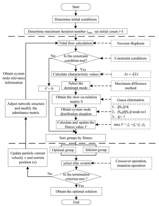
Figure 2. Pseudo-code for solving flow of the GA-IPSO (Asterisks indicate all columns.) (source: plotted by the authors).

(1)

Initialization: Randomly generate the initial positions $x_i$ and velocities $v_i$ of N particles and set their personal-best positions. Among all particles, the best fitness value is taken as the global-best position F. The maximum iteration count $i_{\mathit{max}}$ is also specified.

(2)

Iterative search: loop while $i<i_{\mathit{max}}$:

• Perform power-flow calculation based on the current particle position to obtain system operating information and check whether the solution satisfies all constraints.
• Compute the particle’s fitness value according to the current system state and the objective function.
• Sort particles by fitness, divide the swarm into elite and inferior groups, apply crossover to the elite and mutation to the inferior, then retain the top 50% elites. If the current fitness is better than the historical record, update the personal-best; thereafter refresh the global-best and synchronously update velocity and position.

(3)

Termination and output:

When $i=i_{\mathit{max}}$, the algorithm stops. The global-best position at this moment is the optimal solution to the problem.

5. Simulation Analysis

The simulations were carried out with the PSD-BPA package developed by China Electric Power Research Institute. A ten-machine, 39-bus test system was employed, into which two HVDC links are embedded; the links are terminated at buses 15 and 21, each importing 500 MW. The active splitting model was built in MATLAB 2021a and solved via the YALMIP toolbox with commercial solvers such as Gourbi.

5.1. Comparative Verification Considering HVDC-Stability Constraints

To compare post-splitting voltage stability under different islanding strategies, identical fault conditions are imposed: a three-phase short-circuit is applied to bus 26 and cleared after 25 cycles. All comparative methods are implemented under the same test system, fault scenarios, initial operating points, and simulation tool (PSD-BPA) to ensure comparability.

Figure 3 shows the dynamic response of the system when no controlled islanding is implemented. Without islanding, the grid undergoes large frequency swings and severe voltage sag, threatening secure power supply. In Figure 3, “p.u.” (per unit) denotes the per-unit voltage, defined as the ratio of the actual voltage to the selected voltage base value; it is a dimensionless relative quantity.

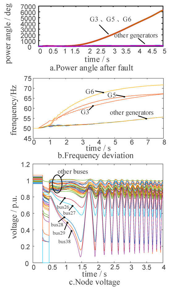
Figure 3. System dynamic data variations without islanding operations: (a) Power angle, (b) Frequency deviation, and (c) Node voltage (source: simulation results of this study).

As shown in Figure 4, after system splitting, both generator rotor angles and bus voltages settle back to steady values. In the frequency traces, Island 1 stabilizes at about 50.23 Hz while Island 2 remains near 49.75 Hz.

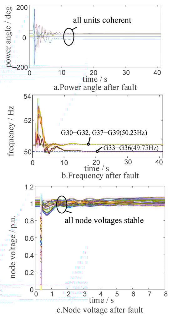
Figure 4. Dynamic system data considering DC stability in scenario one: (a) Power angle, (b) Frequency, and (c) Node voltage (source: simulation results of this study).

Figure 5 displays the splitting surfaces obtained for Scenario 1 with and without the HVDC voltage-stability constraint. The comparison highlights how including this constraint alters the islanding boundary and influences post-splitting system performance.

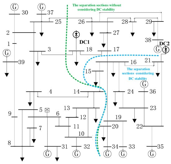
Figure 5. The separation sections considering DC stability in scenario one (The numbers represent bus numbers, and the arrows represent loads.) (source: modified IEEE 39-bus model in this study).

Figure 6 clearly illustrates the critical impact of the HVDC-stability constraint on system voltage excursions. Without the constraint, the voltages of HVDC 1 and HVDC 2 undergo pronounced oscillations; with the constraint, however, the voltages quickly recover after the initial sag and settle within a short time, evidencing a marked gain in robustness.

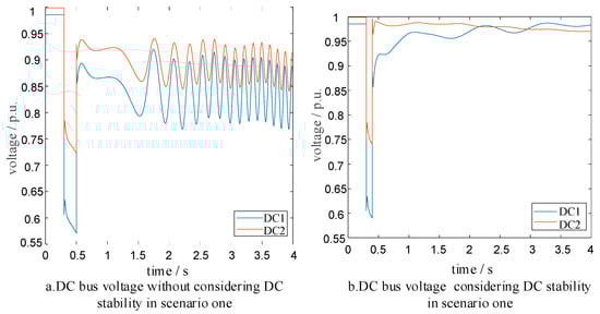
Figure 6. DC bus voltage with/without considering DC stability in scenario one: (a) Without considering DC stability; (b) Considering DC stability (source: simulation results of this study).

When several HVDC links feed the same area, the effective short-circuit capacity drops sharply once the grid is split, pushing the Equivalent Power Index (EPI) downward. This weakens the AC grid’s voltage support to the converter stations and makes voltage instability more likely under certain disturbances. By explicitly embedding the HVDC-stability constraint in the islanding strategy, the post-split subsystems provide stronger voltage support to the DC infeed points even under normal operating conditions. Consequently, severe events such as successive commutation failures are prevented for the same fault scenario, guaranteeing reliable system operation.

Figure 7 compares the extinction-angle variations under the two cases. When the HVDC-stability constraint is taken into account, the extinction angle quickly stabilizes after an initial fluctuation, proving that the constraint noticeably improves extinction-angle stability and reduces the risk of commutation failure. Without considering the HVDC-stability constraint, large swings in the extinction angle raise the probability of commutation failure, which may lead to DC-current interruption and impair normal system operation.

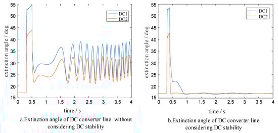
Figure 7. (a,b) Extinction angle of DC converter line in scenario one with/without considering DC stability: (a) Without considering DC stability and (b) Considering DC stability (source: simulation results of this study).

Figure 8 further quantifies the advantage of the islanding strategy that incorporates HVDC-stability constraints. Without these constraints, the highest nodal voltage reaches 1.12 p.u. and the lowest drops to 0.88 p.u., giving a wide voltage excursion band. In contrast, when the splitting surface is chosen by taking the EPI at HVDC feeding points into account, the highest node voltage falls to 1.06 p.u. and the lowest rises to 0.94 p.u., shrinking the overall voltage swing by 28.6%. This result convincingly demonstrates that including HVDC-stability constraints in the selection of the splitting surface strengthens the post-islanding AC subsystems’ voltage support to the HVDC links and thereby improves system voltage stability.

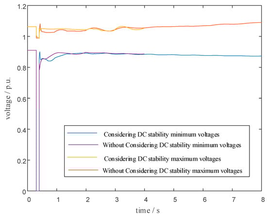
Figure 8. Considering DC stability maximum and minimum voltages in scenario one (source: simulation results of this study).

Table 2 compares the impacts on system stability between the islanding schemes with and without the HVDC-stability constraint. The results show that the EPI-based strategy markedly improves performance. By keeping renewable units in areas of high grid strength and curtailing them in weak regions; the scheme fully exploits their generation capability while preventing reverse-power flows, so the active power balance inside each island is better matched and the flow shock is reduced. With the EPI considered, the flow shock falls from 410.92 MW to 387.41 MW, and the EPI at buses 18 and 21 rises from 1.67 to 5.81 and from 1.39 to 6.22, respectively. A higher EPI means the system is farther from the static voltage-collapse point and possesses a larger stability margin. As the EPI increases, the “equivalent impedance” seen by the load decreases, so the system can deliver reactive power more easily to support voltage, and voltage dips caused by power fluctuations become smaller. In other words, the operating point is pushed away from the voltage-collapse boundary, giving the grid more headroom to withstand load growth or fault disturbances and effectively preventing voltage instability.

Table 2. Power surge considering DC stability (source: simulation results of this study).

In Scenario 1	With Stability Constraints	Without Stability Constraints
Splitting surface	14–15, 16–17	14–15, 3–18, 25–26
Power-flow impact/MW	387.41	410.92
Improved equivalent power index for Node 18	5.81	1.67
Improved equivalent power index for Node 21	6.22	1.39

5.2. Comparison of Results with Different Objective Functions

To ensure comparability, the minimum unbalanced power method in [23] and the minimum power impact method in [24] are implemented under the same test system, fault scenarios, initial operating points, and simulation tool. To further evaluate the performance of different optimization objectives in system splitting strategies, we conduct the same disturbance tests on the modified New England 39-bus system. In Scenario 1, we compare the splitting sections obtained under three different optimization objectives, along with their corresponding power-flow impacts and EPI; the results are presented in Table 3.

Table 3. Decoupling sections and power surge magnitude under different objective functions (source: simulation results of this study).

Objective Function	Splitting Surface	Average EPI Index	Unbalanced Power/MW	Power-Flow Impact/MW
Proposed scheme	14–15, 16–17	6.13	85.73	387.41
Minimum unbalanced power [23]	14–15, 17–18, 26–27	1.57	71.52	453.27
Minimum power-flow impact [24]	6–11, 4–14, 16–17	1.89	113.47	325.17

Table 3 clearly reveals that the three optimization objectives lead to markedly different splitting boundaries and key performance indices. The minimum-flow-shock option in [24] does push the shock down to the lowest value of 325.17 MW, yet its voltage-stability EPI is only 1.89, the worst among all schemes. The minimum-imbalance option in [23] achieves the smallest imbalance of 71.52 MW, but its flow shock soars to 453.27 MW and the EPI drops to 1.57, giving poor results on both counts. By contrast, the proposed maximum-fitness-F strategy delivers a far more balanced and superior profile: specifically, compared with the minimum unbalanced power method in [23], the proposed method increases the voltage stability index from 1.57 to 6.13, representing an improvement of approximately 290%, and reduces the power-flow shock from 453.27 MW to 387.41 MW, a decrease of about 14.5%. Compared with the minimum power impact method in [24], although the proposed method sees a slight increase in power-flow shock, it significantly raises the voltage stability index from 1.89 to 6.13, an improvement of roughly 224%. This indicates that while remarkably enhancing voltage stability, the proposed method maintains both power-flow shock and power imbalance within acceptable ranges, achieving a more balanced comprehensive optimization performance. Furthermore, its flow shock of 387.41 MW is slightly higher than the first scheme and its imbalance marginally above the second, but it offers the best voltage stability. More importantly, the proposed solution requires opening only two lines, whereas the other schemes need three or more. By maximizing F, the method suppresses ambiguous nodes, enlarges the modal-node proportion, and strengthens intra-group relevance while weakening inter-group ties, yielding a crisp and physically coherent partition that better reflects the system’s inherent coherency.

5.3. Comparison of Results Under Different Wind Power Output Scenarios

Table 4 presents the optimal grouping results under different wind power output scenarios. In Scenarios 1 and 2, the system is split into two islands with identical grouping outcomes, whereas in Scenario 3, the system is divided into three islands.

Table 4. Decoupling and clustering results of power systems under different wind power output scenarios (source: simulation results of this study).

Scenario	Number of Clusters	Clustering Result
1	2	{G30, G31, G32, G37, G38, G39} {G33, G34, G35, G36}
2	2	{G30, G31, G32, G37, G38, G39} {G33, G34, G35, G36}
3	3	{G31, G39} {G33, G34, G35, G36} {G30, G32, G37, G38}

The figures in Table 5 show a clear upward trend in flow shock across the splitting surface as wind farm output rises, climbing from 387.41 MW in the first scenario to 430.92 MW and finally 512.51 MW. In Scenarios 1 and 2, the wind farms are located inside Island 1; whenever the system is disturbed and must be split, active power naturally flows from Island 1 toward Island 2. A higher wind generation therefore means more power is pushed across the boundary, so the shock on the tie lines grows markedly. Scenario 3 further amplifies the shock because four lines have to be opened, two more than in the other cases. Examining the fitness value F reveals that Scenarios 1 and 2 share the same splitting surface; the larger the wind output, the smaller F becomes, and in Scenario 2 no alternative line set yields a higher F. Although Scenario 3 offers a surface whose F is slightly below that of Scenario 2, its group structure is more fragmented and requires additional lines to be tripped.

Table 5. Data related to different wind power output scenarios under different wind power output (source: simulation results of this study).

Scenario	Splitting Surface	Power-Flow Impact/MW	Fitness F
1	14–15, 16–17	387.41	2.9376
2	14–15, 16–17	430.92	2.9012
3	1–2, 3–4, 6–11, 4–14	512.51	2.8947

5.4. Parameter Sensitivity Analysis

To verify the robustness and adaptability of the proposed model and algorithm, a sensitivity analysis is conducted on key parameters. The number of Gaussian Mixture Model (GMM) components, the number of clusters, the population size of the particle swarm, and the maximum number of iterations are selected as sensitivity parameters. Their impacts on the objective function (F), average Equivalent Power Index (Avg. EPI), and computation time are evaluated. The parameter ranges are determined based on empirical values and preliminary tests to balance computational efficiency and solution quality.

As shown in Table 6, increasing the number of GMM components from one to three significantly improves both F and EPI—reflecting that multiple components better capture wind power’s multimodal nature—while further increasing to five only brings marginal gains but substantially raises computation time, making three components recommendable; for the number of clusters, increasing from two to three enhances F and EPI (demonstrating that moderate grouping boosts analytical accuracy) yet increasing to four slightly degrades performance and drastically increases computation time, implying over-clustering may cause overfitting; regarding population size and max iterations, increasing both improves solution quality but at a significant computational cost—population size increased from 30 to 50 yields notable improvements with diminishing returns when further raised to 80, and max iterations increased from 50 to 100 greatly enhances results while extending to 200 shows only marginal gains, indicating convergence is largely achieved around 100 iterations.

Table 6. Sensitivity analysis of key parameters (source: simulation results of this study).

Key Parameter	Parameter Range	Impact on Fitness F	Impact on Avg. EPI	Computation Time (s)
No. of Gaussian Components	1 to 3 to 5	2.72 to 2.94 to 2.93	5.48 to 6.13 to 6.10	170.1 to 212.1 to 415.9
No. of Clusters	2 to 3 to 4	2.85 to 2.94 to 2.93	5.35 to 6.13 to 6.08	157 to 212.1 to 455.9
Population Size	30 to 50 to 80	2.79 to 2.94 to 2.95	5.65 to 6.13 to 6.19	251 to 306.4 to 381
Max Iterations	50 to 100 to 200	2.64 to 2.94 to 2.96	5.05 to 6.13 to 6.21	184 to 306.4 to 423.6

5.5. Validation on a Real-World Regional Power System

We have conducted simulation experiments on the Central China Power Grid. However, due to the excessive number of parameters and the unsuitability of displaying geographical wiring diagrams and related data in the paper, we can only present partial content. An N-2 transformer fault was set at the JS node, and islanding was performed according to the proposed method. The voltages of some nodes before and after islanding are shown in Figure 9. The Partial Geographic Wiring Diagram of Central China is shown in Figure 10.

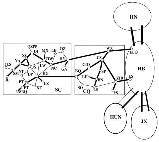
Figure 9. Partial Geographic Connection Diagram of Central China (The thick lines represent the main trunk lines.) (source: draw by authors).

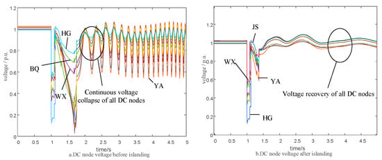
Figure 10. Voltage changes in the Huazhong System before and after islanding: (a) DC node voltage before islanding and (b) DC node voltage after islanding (source: simulation results of this study).

Based on extensive discussions and analysis within our team, we have decided to employ the power grid system developed by the China Electric Power Research Institute for real-world grid analysis. This system represents an actual grid from a specific region in China, with all parameters publicly available, thereby offering greater practical value and facilitating replication by readers, which is more conducive to academic exchange. Its geographical wiring diagram is shown in Figure 11. The system simplifies the grid by equivalencing low-voltage AC nodes, retaining only 500 kV nodes and some 220 kV nodes to maintain simplicity [25].

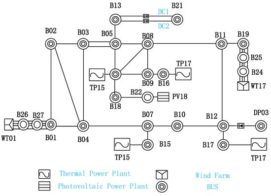
Figure 11. Structure of CSEE-VS (source: redrawn from reference [25]).

This 66-node AC-DC hybrid model—developed for voltage stability analysis based on Chinese engineering practice—aligns closely with our research scope: over 50% of its total capacity comes from 1.2 MW PV and 2.4 MW wind power, it features a dual-circuit 1600 MW multi-infeed HVDC system connected to bus B13, and its topology/parameters are practical (complete parameters in Appendix A). A three-phase short-circuit fault is set at the midpoint (50%) of the B01-B04 line. All methods use the same pre-fault conditions: electromechanical transient simulations via PSD-BPA, and the optimization model (built in MATLAB) solved by the GA-IPSO algorithm.

Figure 12 illustrates the dynamic recovery of key bus voltages after the fault. As shown, without islanding, the system voltage continues to decline, eventually leading to voltage collapse. After employing the proposed islanding method, all bus voltages recover rapidly to above 0.95 p.u. within 2 s and remain stable. Following islanding operation, voltages at critical nodes such as B07, B08, and B11 quickly recover and stabilize around 1.0 p.u., demonstrating the effectiveness of the proposed method in restoring voltage stability in practical systems.

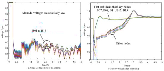
Figure 12. Voltage changes in the CSEE-VS system before and after islanding: (a) Node voltage before islanding and (b) Node voltage after islanding (source: simulation results of this study).

Figure 13 highlights the changes in DC bus voltage before and after islanding, with a rated voltage of 500 kV. Without implementing the islanding strategy, the DC bus voltage continuously declines after the fault, ultimately leading to DC block. In contrast, with the proposed method, the DC bus voltage rapidly recovers after a brief dip, returning to above 0.96 p.u. within 2.5 s and maintaining stability thereafter.

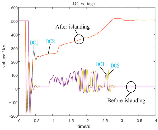
Figure 13. DC voltage before and after islanding.

6. Conclusions

This paper addresses the active islanding problem in power systems with high-penetration renewables and multiple HVDC infeed by proposing a splitting-surface optimization model that simultaneously accounts for wind power uncertainty and multi-infeed DC voltage stability. Through theoretical modeling, algorithm enhancement, and simulation verification, the main conclusions corresponding to the research objectives are drawn as follows:

• Regarding the modeling of wind power uncertainty, the proposed GMM-K-means scenario generation and reduction method effectively captures the multimodal distribution characteristic of wind generation. The resulting representative scenario set significantly improves the model’s adaptability to wind power randomness while maintaining computational efficiency, thereby overcoming the insufficient consideration of wind uncertainty in existing methods.
• Regarding the enhancement of post-splitting voltage stability, the introduction of the Improved Equivalent Power Index (IEPI) into the optimization model prevents multiple HVDC feeding points from being concentrated in islands with weak voltage support capability. Simulation results demonstrate that compared with schemes without HVDC-stability constraints, the proposed method reduces the system voltage fluctuation range and moves the operating point farther away from the voltage-collapse boundary, substantially enhancing the voltage stability margin of islands.
• Regarding the solution of the complex optimization model, the proposed genetic-inspired improved particle swarm optimization (GA-IPSO) algorithm, incorporating a “grouping-screening-evolution” mechanism, reliably solves the high-dimensional nonlinear problem. It effectively balances global exploration and local exploitation, suppressing premature convergence and offering a robust solver for the intricate splitting-surface search.
• Regarding the comprehensive validation of the proposed framework, simulations conducted on the modified New England 39-bus system confirm its overall superiority. Compared to traditional methods that prioritize minimum power imbalance or minimum power-flow shock, the proposed scheme achieves the optimal voltage stability—with an average Equivalent Power Index (EPI) improvement of approximately 290% over the minimum imbalance method. Meanwhile, it effectively controls key indicators within acceptable ranges: the power-flow shock is reduced from 453.27 MW to 387.41 MW (a decrease of about 14.5%), and power imbalance is well managed. This fully demonstrates the scheme’s stronger comprehensive optimization capability, making it more suitable for practical active islanding applications.

References

- Alhelou, H.H.; Hamedani-Golshan, M.E.; Njenda, T.C.; Siano, P. A Survey on Power System Blackout and Cascading Events: Research Motivations and Challenges. Energies 2019, 12, 682. [Google Scholar] [CrossRef]
- Hessan, E.; Roy, S.; Mohammad, N.; Nawar, N.; Ditta, D.R. Metrics and enhancement strategies for grid resilience and reliability during natural disasters. Appl. Energy 2021, 290, 116709. [Google Scholar] [CrossRef]
- Xue, Y. Space-time cooperative framework for defending blackouts part III optimization and coordination of defense-lines. Autom. Electr. Power Syst. 2006, 30, 8–16. (In Chinese) [Google Scholar]
- Kyriacou, A.; Demetriou, P.; Panayiotou, C.; Kyriakides, E. Controlled islanding solution for large-scale power systems. IEEE Trans. Power Syst. 2018, 33, 1591–1602. [Google Scholar] [CrossRef]
- Sen, A.; Ghosh, P.; Vittal, V.; Yang, B. A new min-cut problem with application to electric power network partitioning. Eur. Trans. Electr. Power 2009, 19, 778–797. [Google Scholar] [CrossRef]
- Wang, C.G.; Zhang, B.H.; Hao, Z.G.; Shu, J.; Li, P.; Bo, Z.Q. A novel real-time searching method for power system splitting boundary. IEEE Trans. Power Syst. 2010, 25, 1902–1909. [Google Scholar] [CrossRef]
- Wang, X. Slow Coherency Grouping Based Islanding Using Minimal Cutsets and Generator Coherency Index Tracing Using Thecontinuation Method. Ph.D. Thesis, Iowa State University, Ames, Iowa, 2005. [Google Scholar]
- Sun, K.; Zheng, D.; Lu, Q. Splitting strategies forislanding operation of large-scale power systems using OBDD-based methods. IEEE Trans. Power Syst. 2003, 18, 912–923. [Google Scholar] [CrossRef]
- Aghamohammadi, M.R.; Shahmohammadi, A. Intentional islanding using a new algorithm based on ant search mechanism. Int. J. Electr. Power Energy Syst. 2012, 35, 138–147. [Google Scholar] [CrossRef]
- Fan, N.; Izraelevitz, D.; Pan, F.; Pardalos, P.M.; Wang, J. A mixed integerprogramming approach for optimal power grid intentional islanding. Energy Syst. 2012, 3, 77–93. [Google Scholar] [CrossRef]
- Amraee, T.; Saberi, H. Controlled islanding using transmission switching and load shedding for enhancing power grid resilience. Int. J. Electr. Power Energy Syst. 2017, 91, 135–143. [Google Scholar] [CrossRef]
- Teymouri, F.; Amraee, T. An MILP formulation for controlledislanding coordinated with under frequeny load shedding plan. Electr. Power Syst. Res. 2019, 171, 116–126. [Google Scholar] [CrossRef]
- Teymouri, F.; Amraee, T.; Saberi, H.; Capitanescu, F. Toward controlled islanding for enhancing power grid resilience considering frequency stability constraints. IEEE Trans. Smart Grid 2019, 10, 1735–1746. [Google Scholar] [CrossRef]
- Muñoz, J.; Tipán, L.; Cuji, C.; Jaramillo, M. Resilient Distribution System Reconfiguration Based on Genetic Algorithms Considering Load Margin and Contingencies. Energies 2025, 18, 2889. [Google Scholar] [CrossRef]
- Ni, J.; Shen, C.; Chen, Q. Adaptive controlled islanding based on slow coherency (Part I): Theoretical foundation. Proc. CSEE 2014, 34, 4374–4384. (In Chinese) [Google Scholar]
- Ni, J.; Shen, C.; Chen, Q. Adaptive controlled islanding based on slow coherency (Part II): Practical slow coherency grouping method. Proc. CSEE 2014, 34, 4865–4875. (In Chinese) [Google Scholar]
- Yang, F.; Fu, X.; Li, Z.; Qiu, D.; Hamed, B. A novel clustering-ensemble learning model for day-ahead photovoltaic power forecasting. Eng. Appl. Artif. Intell. 2025, 161, 112281. [Google Scholar] [CrossRef]
- Shukla, A.; Singh, S.N. Clustering based unit commitment with wind power uncertainty. Energy Convers. Manag. 2016, 111, 89–102. [Google Scholar] [CrossRef]
- Tyuryukanov, I.; Bos, J.A.; van der Meijden, M.A.; Terzija, V.; Popov, M. Controlled Power System Separation Using Generator PMU Data and System Kinetic Energy. IEEE Trans. Power Deliv. 2023, 38, 2618–2629. [Google Scholar] [CrossRef]
- Ma, J.; Zeng, Y.; Sheng, H.; Zhang, Z. Static voltage stability assessment method based on equivalent power index. Power Syst. Technol. 2025, 49, 2347–2355. (In Chinese) [Google Scholar]
- Fachini, F.; Bogodorova, T.; Vanfretti, L.; Boersma, S. A microgrid control scheme for islanded operation and re-synchronization utilizing Model Predictive Control. Sustain. Energy Grids Netw. 2024, 39, 101464. [Google Scholar] [CrossRef]
- Shi, H.; Fan, C.; Bin, F.; Wang, Y.; Chen, Z.; Chen, G. Optimal Controlled Islanding Method Considering Frequency Stability Constraints. In Proceedings of the 2022 4th International Conference on Power and Energy Technology (ICPET), Beijing, China, 28–31 July 2022; pp. 1237–1243. [Google Scholar]
- Qiao, Y.; Shen, C.; Lu, Q. Decision space reduction and fast search method for power system islanding. Proc. CSEE 2008, 28, 23–28. (In Chinese) [Google Scholar]
- Wu, X.; He, L.; Li, Y.; Shuai, Z. Analysis of the impact of grid impedance and PLL coupling effects on stability of grid-connected MMC system under weak grid conditions. Trans. China Electrotech. Soc. 2025, 40, 1236–1253. [Google Scholar]
- Wang, X.; Zhao, B.; Wu, P.; Xu, S.; Xi, G.; Wang, L.; Wang, D. Benchmark for AC-DC Hybrid System With High Penetration of Renewables (III): Voltage Stability CSEE-VS. Proc. CSEE 2024, 44, 8353–8363. (In Chinese) [Google Scholar]
Disclaimer/Publisher’s Note: The statements, opinions and data contained in all publications are solely those of the individual author(s) and contributor(s) and not of MDPI and/or the editor(s). MDPI and/or the editor(s) disclaim responsibility for any injury to people or property resulting from any ideas, methods, instructions or products referred to in the content. |
© 2025 by the authors. Licensee MDPI, Basel, Switzerland. This article is an open access article distributed under the terms and conditions of the Creative Commons Attribution (CC BY) license.