Towards Sustainable Intelligent Transportation Systems: A Hierarchical Spatiotemporal Graph–Hypergraph Network for Urban Traffic Flow Prediction

Abstract

Spatiotemporal traffic flow prediction is a fundamental task in intelligent transportation systems and is crucial for promoting efficient and sustainable urban mobility, especially under increasingly complex and rapidly evolving traffic conditions. To overcome the challenges of modeling high-order spatial dependencies and heterogeneous temporal patterns, this study develops a novel Hierarchical Spatiotemporal Graph–Hypergraph Network (HSTGHN). For spatial representation learning, a hypergraph neural module is employed to capture high-order interactions across the road network, while a hypernode mechanism is designed to characterize complex correlations among multiple road segments. Furthermore, an adaptive adjacency matrix is constructed in a data-driven manner and enriched with prior knowledge of bidirectional traffic flows, thereby enhancing the robustness and accuracy of graph structural representations. For temporal modeling, HSTGHN integrates the complementary strengths of Gated Recurrent Units (GRUs) and Transformers: GRUs effectively capture local sequential dependencies, whereas Transformers excel at modeling global dynamic patterns. This joint mechanism enables comprehensive learning of both short-term and long-term temporal dependencies. Extensive experiments on multiple benchmark datasets demonstrate that HSTGHN consistently outperforms state-of-the-art baselines in terms of prediction accuracy and stability, with particularly significant improvements in long-term forecasting and highly dynamic traffic scenarios. These improvements provide more reliable decision support for intelligent transportation systems, contributing to enhanced traffic efficiency, reduced congestion, and ultimately more sustainable urban mobility.

1. Introduction

With the accelerating pace of global urbanization, the rapid growth of urban populations has posed severe challenges to traffic management and environmental sustainability. As a core function of intelligent transportation systems (ITS), traffic flow prediction aims to provide accurate short-term and long-term forecasts of future traffic conditions. Reliable and robust traffic flow forecasting plays a critical role in enabling proactive traffic management, mitigating congestion, and improving road safety [1,2]. However, due to the increasing complexity of urban road networks and the combined effects of nonlinear factors such as traffic accidents and adverse weather, as well as highly dynamic spatiotemporal correlations, traffic flow prediction faces numerous challenges, including accuracy degradation over time and the difficulty of modeling intricate spatiotemporal dependencies [3].

In the early stages of research, traffic flow prediction was primarily regarded as a multivariate time series forecasting problem and mainly relied on statistical approaches such as the Autoregressive Integrated Moving Average (ARIMA) model [4,5] and the Markov model [6]. While these methods performed well for short-term stationary time series, their strong stationarity assumptions meant they struggled to capture the complex nonlinear dynamics and spatiotemporal interactions inherent in traffic flows effectively. With the development of machine learning, time series methods such as Support Vector Regression (SVR) [7] and Random Forest (RF) [8] introduced nonlinear modeling capabilities, thereby significantly improving prediction accuracy. Nevertheless, early studies generally considered only temporal features, leaving the dynamic spatial correlations among road network nodes insufficiently represented. More recently, the emergence of deep learning has brought new breakthroughs to traffic flow forecasting [9]. Methods based on Recurrent Neural Networks (RNNs) and their variants, such as Long Short-Term Memory (LSTM) and Gated Recurrent Unit (GRU) [10], as well as Temporal Convolutional Networks (TCNs) [11], have demonstrated superior performance in time series modeling. Recent studies [12,13,14] further demonstrate the effectiveness of RNN-based approaches for time series analysis. These models effectively capture temporal dependencies, and when combined with Convolutional Neural Networks (CNNs), they can jointly model spatiotemporal patterns in traffic flows. However, CNNs are designed for Euclidean-structured data with regular grid topologies, making them well-suited for tasks like image analysis. Urban road networks exhibit non-Euclidean structures with irregular topological relationships that cannot be effectively captured by standard grid convolutions, thus limiting spatial feature extraction.

With the advent of graph neural networks (GNNs), traffic flow forecasting has entered a new paradigm. Researchers frequently integrate GNNs with recurrent architectures such as RNNs or LSTMs to construct spatiotemporal prediction models. Among GNN variants, the graph convolutional network (GCN) is considered particularly suitable for modeling the spatial dependencies of urban traffic systems. GCNs effectively capture intricate dependencies embedded in non-Euclidean space by representing road networks as graph structures, where nodes correspond to road segments or intersections and edges capture their connections. GCN-based models [15,16,17] have achieved significant performance improvements by integrating spatial correlations with temporal sequence modeling for traffic flow forecasting. These approaches have demonstrated state-of-the-art results across multiple public datasets and benchmark tests. Nevertheless, existing graph-based models still face several limitations. Most approaches emphasize pairwise node interactions (i.e., edge-level dependencies), while overlooking the higher-order interactions among multiple road segments or regions that frequently arise in real-world traffic systems. Furthermore, the dynamic nature of traffic flows, external influences (e.g., weather and special events), and long-term error accumulation present substantial modeling challenges. Therefore, there is a pressing need for more advanced frameworks capable of capturing higher-order spatiotemporal interactions and enhancing both the robustness and accuracy of traffic flow prediction.

To address the limitations of existing traffic flow forecasting models in capturing high-order spatiotemporal interactions and dynamic evolution characteristics, this paper proposes a novel Hierarchical Spatiotemporal Graph–Hypergraph Network (HSTGHN) framework. Unlike traditional graph convolutional networks [17,18,19] that model pairwise relationships, the proposed approach employs hypergraph-based modules to represent complex multidimensional traffic patterns more effectively. Moreover, most graph-based models rely on static or predefined structures, limiting their adaptability to evolving traffic conditions. We develop an attention-based mechanism that adaptively constructs time-varying hypergraph structures in response to dynamic traffic patterns. Additionally, we integrate Transformer and GRU architectures to enhance temporal modeling. This hybrid approach significantly improves forecasting accuracy and robustness in complex traffic scenarios.

The proposed HSTGHN model is designed to provide reliable traffic forecasts and demonstrates strong practical value for real-world traffic management. It can predict traffic flow and speed across multiple urban networks, making it suitable for urban traffic control, signal optimization, and congestion prediction. By offering timely traffic information, the model enables transportation authorities to enhance traffic efficiency, reduce congestion, and support sustainable urban mobility through lower emissions and energy consumption.

Building on these motivations, this study presents the HSTGHN framework to tackle the spatiotemporal modeling challenges inherent in traffic flow prediction. The main contributions of this study are as follows:

• We introduce a hypergraph neural network module to capture high-order interactions in traffic networks. Leveraging a hypernode mechanism, the model effectively represents complex correlations among multiple road segments, while a data-driven adaptive adjacency matrix with forward and backward traffic flow priors enhances the accuracy and robustness of spatial representations.
• By combining the complementary strengths of GRU and Transformer, the model jointly captures short-term and long-term temporal dependencies, enabling more effective prediction under complex temporal structures.
• Extensive experiments on multiple benchmark datasets show that HSTGHN consistently outperforms state-of-the-art baselines in both predictive accuracy and stability, with particularly strong improvements in long-term forecasting and dynamic traffic scenarios.

2. Related Works

2.1. Graph Convolutional Networks and Hypergraph Convolutional Networks

Bruna et al. were the first to introduce spectral graph theory into deep learning by leveraging the eigendecomposition of the graph Laplacian matrix, projecting graph signals into the spectral domain [20]. In their framework, a parameterized diagonal matrix was employed to simulate the convolutional kernels in conventional CNNs. However, the explicit eigendecomposition makes this approach computationally impractical for large-scale or dynamic graphs. To overcome this limitation, Defferrard et al. proposed approximating spectral graph convolution using Chebyshev polynomials of various orders [21]. This method assumes that the representation of a central node depends on its higher-order neighbors, thereby ensuring a strictly localized receptive field in the spatial domain. It avoids costly eigendecomposition and exhibits efficiency, locality, and improved parameter optimization. Nonetheless, its performance is still constrained by the choice of polynomial order and associated precomputation costs. Kipf further simplified this formulation by introducing a first-order approximation, leading to the classical GCN model [16]. This model efficiently integrates node features with graph diffusion processes, reduces computational complexity, and incorporates self-connections and symmetric normalization into the adjacency matrix, thereby improving stability. Importantly, it has provided a solid theoretical foundation for subsequent GCN-based research. Later, Hamilton et al. observed that GCNs incur significant memory consumption when applied to large-scale graphs [22]. To address this issue, they proposed the GraphSAGE model, which leverages both node features and structural information by sampling and aggregating features from a node’s local neighborhood to generate graph embeddings. This approach is particularly advantageous for handling dynamic graphs, large-scale networks, and real-world scenarios with continuous node additions.

Traditional GCNs [17,23,24] primarily capture pairwise node relationships, limiting their ability to model high-order spatial dependencies that involve multiple nodes. Hypergraph convolutional networks (HGCNs) extend GCNs by introducing hyperedges that simultaneously connect arbitrary sets of nodes, enabling explicit modeling of complex higher-order interactions [25,26]. This architecture is particularly advantageous in scenarios with prevalent multi-node dependencies, such as coordinated traffic flows [27], multi-path coupling [28], and collective congestion dynamics [29]. Central to HGCNs is the bidirectional message-passing mechanism between nodes and hyperedges, which effectively extracts group-level structural features beyond the reach of conventional GCNs. To further enhance their representational capacity, recent approaches incorporate adaptive hyperedge construction [30], attention-based node–hyperedge weighting [31], and dynamic hypergraph modeling [32], improving sensitivity to latent correlations and adaptability to non-stationary spatiotemporal dependencies. In urban traffic networks, HGCNs are well-suited to reveal collective dependencies among multiple road segments. For example, models such as DDSTGCN [33] exploit dynamic hyperedge correlations to uncover intricate latent relationships, capturing multi-path traffic interactions and flow evolution more comprehensively. Dynamic spatiotemporal HGCNs introduce joint graph–hypergraph learning with adaptive hyperedge refinement, enabling more accurate modeling of evolving traffic structures [34]. Residual HGCN architectures alleviate over-smoothing through residual connectivity, improving the extraction of global spatiotemporal features [35]. Compared with pairwise graph-based methods, HGCNs exhibit superior capability in representing the complexity and high coupling inherent in urban traffic systems, offering a robust framework for traffic forecasting, resilience assessment, and intelligent traffic management [36]. Their capacity to encode higher-order dependencies and adaptively learn structural patterns positions HGCNs as a pivotal paradigm in advancing data-driven urban transportation modeling.

2.2. Graph Structure Learning

Graph structure learning plays a crucial role in graph neural networks. Early GCN models generally rely on static adjacency matrices, where node relationships are typically defined by physical connectivity or spatial distance [23]. However, such static constructions are limited in that they cannot capture latent spatiotemporal dependencies between non-adjacent nodes. To address this issue, some studies have explored data-driven approaches to construct adaptive graphs that learn implicit spatial relationships among nodes [37]. Nevertheless, once trained, the learned adaptive graph remains fixed, making it incapable of reflecting the dynamic evolution of road networks. Consequently, researchers have investigated dynamic graph construction to adapt to structural variations in traffic networks [18,38]. Benefiting from the powerful representation capacity of Transformer models in natural language processing [39] and computer vision [40], recent studies often integrate attention mechanisms into GNNs [18,41]. For example, MegaCRN [42] proposes a meta-graph learner that explicitly separates spatiotemporal heterogeneity and builds dynamic graph structures from observational data. This design allows the model to capture traffic flow evolution more effectively, particularly during transitions from stable to non-stationary conditions. Overall, graph structure learning has progressed from static adjacency matrices to adaptive and dynamic graph modeling. In the domain of traffic forecasting, an important trend lies in combining graph structure learning with time series modeling techniques, which opens up broad opportunities for future research [1].

2.3. Spatiotemporal Traffic Flow Forecasting

In spatiotemporal traffic flow research, DCRNN [23] was the first to integrate diffusion convolution with gated recurrent units (GRU), leveraging GCNs with bidirectional random walks on graphs to capture spatial dependencies while using GRUs to model temporal dynamics. This effectively addressed the limitations of traditional time series prediction models [43], which struggle to simultaneously capture complex spatial dependencies and nonlinear temporal patterns. However, RNN-based models rely on sequential propagation of temporal information, leading to significant computational overhead for long sequences compared with CNN-based approaches. To address this, STGCN [44] replaced RNN structures with gated temporal convolutions (Gated-TCN) for temporal feature extraction, combined with GCNs to effectively capture spatiotemporal features of traffic data, thereby improving computational efficiency. ASTGCN [15] innovatively incorporated spatiotemporal attention mechanisms with periodic dependencies and leveraged GCNs alongside standard convolutions to extract spatiotemporal features, significantly enhancing traffic flow prediction accuracy. For large-scale traffic datasets, some studies have proposed replacing STGNN models with spatiotemporal multilayer perceptrons, achieving competitive prediction accuracy with reduced computational resources and inference time [45]. Graph Wavenet [37] introduced adaptive adjacency matrices combined with gated temporal convolutions, employing gating mechanisms to handle temporal dependencies and adaptive graph construction to model spatial correlations. Benefiting from the powerful representational capacity of attention mechanisms, GMAN [46] employed multi-head spatiotemporal attention to dynamically learn spatial correlations and temporal dependencies, substantially improving long-term prediction accuracy while mitigating the sensitivity to error propagation inherent in traditional GNNs. Recently, researchers have increasingly adopted models integrating graph neural networks with attention mechanisms for traffic flow prediction, further improving performance on public datasets such as PEMS and METR-LA [38,41,47]. Wang et al. [48] encoded recent, weekly, and monthly traffic flow features during data preprocessing and employed Transformer modules to extract temporal features, complemented by GATs for spatial feature extraction. Han et al. [49] utilized attention mechanisms to learn temporal features, quantified spatial dependencies through attention scoring, and combined a linear feature extractor to encode data into low-dimensional representations, suitable for large-scale road networks.

3. Method

3.1. Overview

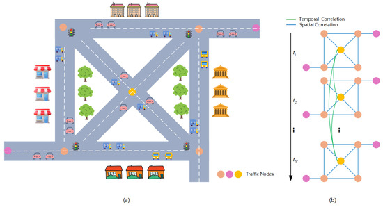
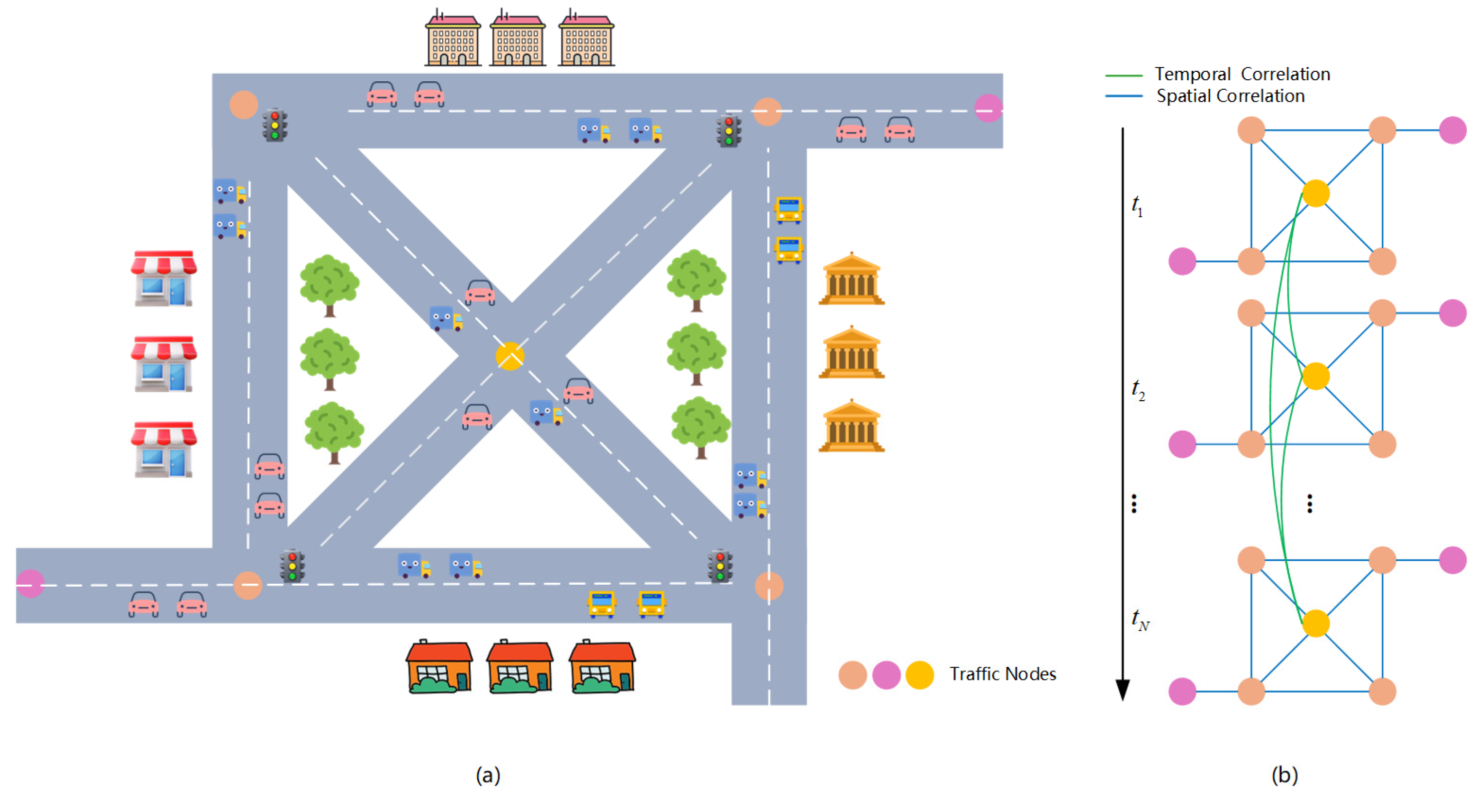
Traffic Network Representation. Urban traffic networks exhibit complex spatiotemporal characteristics, as illustrated in Figure 1. Each node represents an intersection or road segment, while edges capture spatial correlations between adjacent locations. The spatiotemporal graph structure integrates spatial dependencies through horizontal connections and temporal evolution through vertical links, providing a comprehensive framework for modeling traffic dynamics.

Figure 1. Urban traffic network and spatiotemporal correlation. (a) Road network with traffic nodes representing intersections or road segments. (b) Spatiotemporal graph where horizontal edges denote spatial correlations and vertical edges capture temporal dependencies.

Problem Definition. Our objective is to predict the future traffic flow of the road network based on historical traffic data. Accordingly, the problem can be formally defined as follows.

$$[X^{(t-T^{\prime }+1)},\dots ,X^{(t)};G]\stackrel{h(\cdot )}{\to }[X^{(t+1)},\dots ,X^{(t+T)}]$$

(1)

Let $X$ denote the traffic flow data, where $X^t$ represents the traffic flow of the road network at time step $t$. The road network is represented as a directed, weighted graph $G=(V,E,A)$, where $V$ is the set of sensor nodes with $\left|V\right|=N$, $E$ is the set of edges, and $A\in R^{N\times N}$ is the adjacency matrix, with elements indicating edge connectivity or weights. Let $T^{\prime }$ denote the length of the historical traffic flow sequence input to the model, and $T$ denote the length of the future traffic flow sequence to be predicted. Finally, $h(\cdot )$ represents the mapping function from historical to future traffic flow.

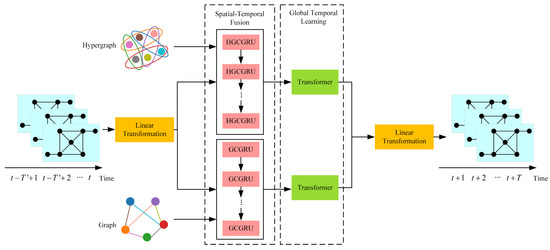
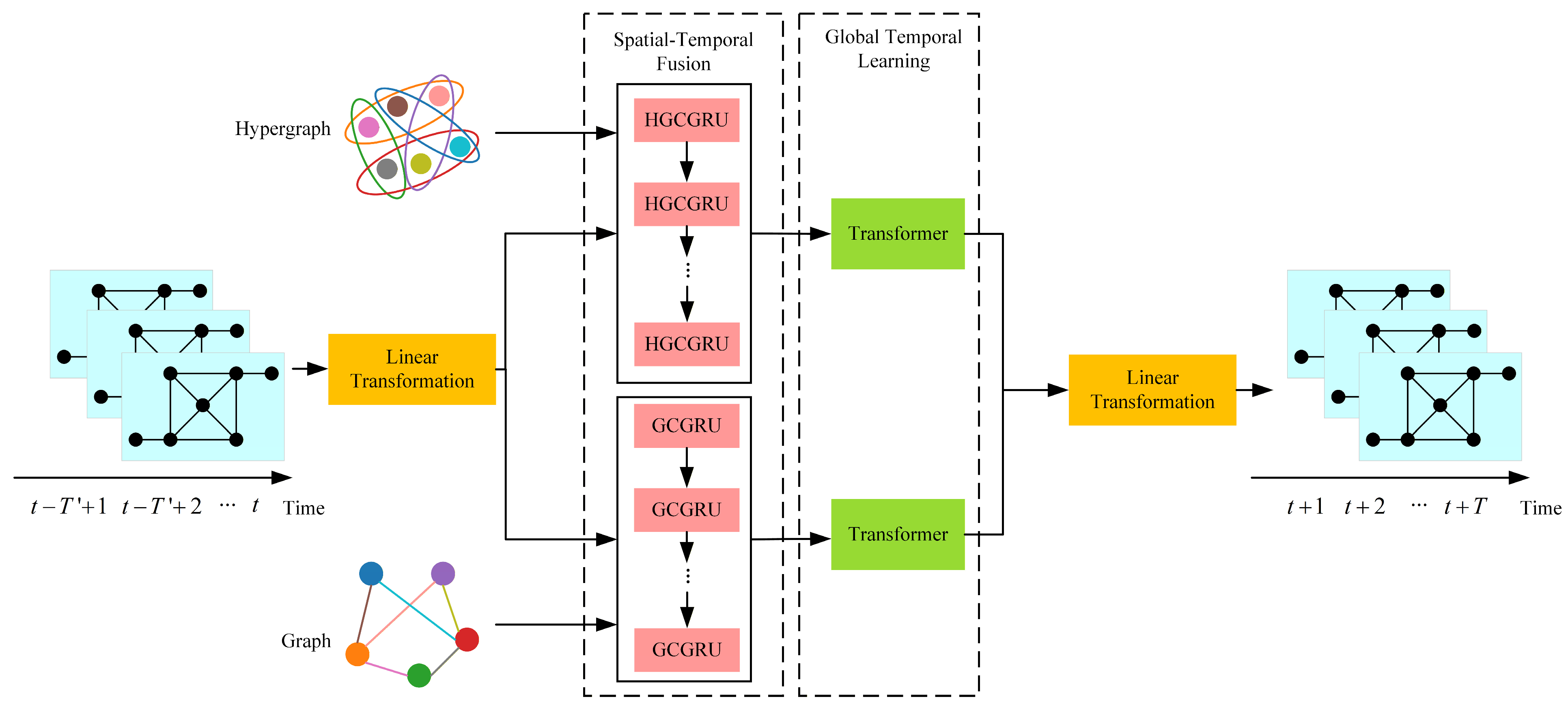
Framework. In this study, we propose the HSTGHN model, the overall architecture of which is presented in Figure 2. The framework is organized into two fundamental components, including a spatial–temporal fusion module and a global temporal learning module. First, spatial–temporal traffic flow data are projected into a high-dimensional feature space through a linear transformation, thereby enhancing feature representation. The transformed data are subsequently partitioned into two parallel streams and processed by the Graph Convolutional Gated Recurrent Unit (GCGRU) and Hypergraph Convolutional Gated Recurrent Unit (HCGRU) modules to capture hierarchical spatial–temporal dependencies among road nodes and segments. The extracted features are then fed into a Transformer module, which models long-range temporal correlations while incorporating the latent spatial–temporal dependencies learned in the fusion stage. Finally, another linear transformation is applied to map the learned representations into the target output space, generating the final traffic predictions. The detailed designs of each module are elaborated in the following subsections.

Figure 2. Overall Framework of the HSTGHN Model.

3.2. Dynamic Spatial Dependency Modeling via Graph–Hypergraph Fusion

In this section, we propose a graph–hypergraph fusion module for spatiotemporal feature extraction in traffic flow modeling. The module consists of two parallel components: GCGRU and HCGRU. Specifically, GCGRU is designed to capture the spatiotemporal features of road nodes, while HCGRU focuses on extracting the spatiotemporal dependencies among road segments. Subsequently, the features from each branch are processed by independent Transformer modules and fused through a Linear Transformation layer, thereby yielding a comprehensive representation of the dynamic spatial dependencies within the road network.

3.2.1. High-Order Spatial Dependency Modeling via Hypergraph Convolution

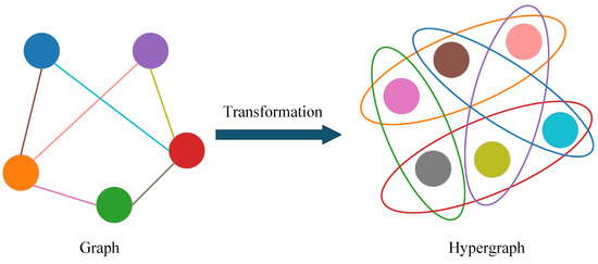
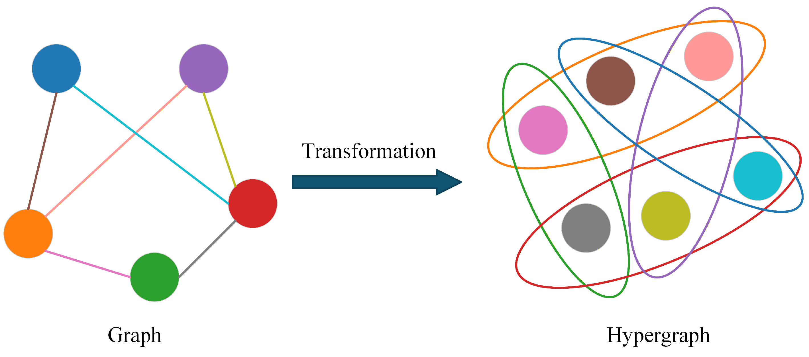
GCNs primarily rely on adjacency matrices to capture first-order or second-order neighborhood relations, which makes them inadequate for modeling the complex multi-segment interactions commonly observed in traffic networks. To address this limitation, we introduce the concept of hypergraph learning, wherein a graph–hypergraph dual transformation is employed to map graph nodes into hyperedges and graph edges into hypernodes, as illustrated in Figure 3. Building on this foundation, we design a hypergraph convolution module within the HCGRU structure to model high-order dependencies among road segments. By constructing hyperedges that simultaneously connect multiple nodes, the proposed module enables group-level feature aggregation, thereby offering a more effective representation of intricate spatial dependency patterns.

Figure 3. Graph-to-Hypergraph Dual Transformation.

Construction of Hypernode Features. Let the transportation network consist of a node set $\mathcal{V}=\{v_1,v_2,\dots ,v_N\}$, and denote its hypergraph representation as $\mathcal{H}=(\mathcal{V},\mathcal{E})$. In this framework, each hyperedge $e\in \mathcal{E}$ is capable of encompassing multiple nodes. The hypergraph incidence matrix is defined as follows.

$$H(v,e)=\left\{\begin{array}{c}1,if{v}_i\in e_j\\ 0,otherwise\end{array}\right.$$

(2)

Here, $H\in {ℝ}^{E\times N}$ denotes the incidence matrix, which encodes the structural information of the road network. Considering that traffic flow networks are typically directed graphs, we decompose the constructed incidence matrix $H$ into $H_f\in {ℝ}^{E\times N}$ and $H_b\in {ℝ}^{E\times N}$ to represent the forward and backward connectivity within the road network, respectively.

Since the edges in a traffic network inherently carry dynamic correlations among road segment nodes, we incorporate edge-based prior information from traffic flow into the node features of the graph to construct the hypernode features $X_h$ for the hypergraph.

$$X_h=Concat(W_f\odot H_{f}X,W_b\odot H_{b}X,L_{dis})$$

(3)

Here, $X_h\in {ℝ}^{E\times (2C+1)\times T}$ denotes the hypernode features, and $L_{dis}\in {ℝ}^E$ represents the edge distance matrix, where each element encodes the length attribute of the corresponding edge.

Hypergraph Convolution. Building on this, we can define the information propagation rule for hypergraph convolution as follows.

$${{\tilde{X}}_h}^{\prime }=\sigma \left(D_v^{-{\displaystyle \frac{1}{2}}}H{W}_e{D}_e^{-1}{H}^{\top }{D}_v^{-{\displaystyle \frac{1}{2}}}{\tilde{X}}_h{\mathsf{\Theta }}_h\right)$$

(4)

Here, ${\tilde{X}}_h\in {ℝ}^{\mathrm{E}\times C_1}$ denotes the input features of the hypernodes, $H\in {ℝ}^{E\times N}$ is the hypergraph incidence matrix, $D_v\in {ℝ}^{\mathrm{E}\times E}$ and $D_e\in {ℝ}^{N\times N}$ represent the degree matrices of hypernodes and hyperedges, respectively, $W_e\in {ℝ}^{N\times N}$ is a learnable hyperedge weight matrix that is dynamically adjusted via backpropagation to emphasize the contribution of critical hyperedges, ${\mathsf{\Theta }}_h\in {ℝ}^{C_1\times C_2}$ is a learnable parameter matrix, $\sigma (\cdot )$ is a nonlinear activation function, and ${{\tilde{X}}_h}^{\prime }\in {ℝ}^{\mathrm{E}\times C_2}$ represents the updated node feature matrix. Through the hypergraph convolution module, nodes engage in high-order interactions via hyperedges, thereby capturing the complex dependencies among road segments.

Finally, the hypernode features are mapped back to the original graph node representations using learnable parameters, and a linear transformation is applied to project the data back to its original feature dimension. This process can be formally expressed as follows.

$${\tilde{X}}_h=W_h{X}_h^{\prime }$$

(5)

Here, $W_h\in {ℝ}^{N\times E}$ denotes a learnable parameter used to map the hypergraph-structured features back to the original graph structure, yielding the output ${\tilde{X}}_h\in {ℝ}^{N\times C_2}$ of the module.

3.2.2. Adaptive Graph Structure Learning

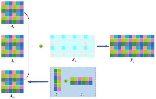
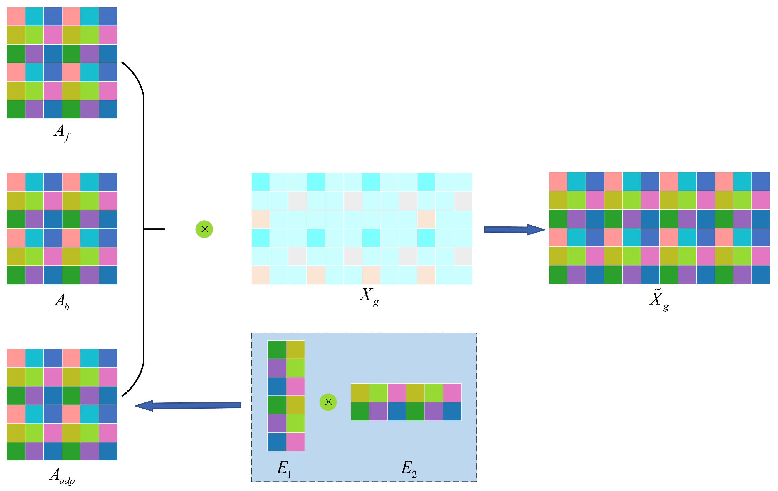
To more effectively capture the spatial dependencies among nodes, we integrate a data-driven adaptive graph generation mechanism into the GCGRU module, enabling the dynamic construction of the adjacency matrix. In particular, the adjacency matrix is trainable and is derived from randomly initialized node embedding matrices. This matrix is continuously optimized during training, thereby uncovering implicit traffic dependencies that cannot be explicitly characterized by the underlying physical topology. The process of constructing the adaptive adjacency matrix can be expressed as follows.

$$A_{adp}=softmax(relu(E_1{E}_2^{\mathrm{T}}))$$

(6)

Here, $E_1\in {ℝ}^{N\times d_e}$ and $E_2\in {ℝ}^{N\times d_e}$ denote the randomly initialized node embedding matrices, while $A_{adp}$ represents the adaptive adjacency matrix, which can be automatically learned and updated during training to capture latent traffic dependencies that are difficult to explicitly represent in the original physical topology. The function $softmax(\cdot )$ is employed to normalize the adaptive matrix, ensuring numerical stability and enhancing the interpretability of spatial relationships.

On this basis, we further incorporate static adjacency matrices constructed from prior knowledge, including both the forward and backward adjacency matrices. These matrices are designed to capture the road network’s connectivity and bidirectional interaction dependencies, thereby compensating, to some extent, for the potential uncertainties of the adaptive adjacency matrix during training. The graph convolution process, after integrating these three types of adjacency matrices, can be formally expressed as follows.

$${\tilde{X}}_g^k=\sigma \left(A_f{X}^k{\mathsf{\Theta }}_f^k+A_b{X}^k{\mathsf{\Theta }}_b^k+A_{adp}{X}^k{\mathsf{\Theta }}_{adp}^k\right)$$

(7)

Here, $A_f$ and $A_b$ denote the static adjacency matrices constructed based on physical distance or connectivity, which capture the spatial interaction features of traffic flows in the forward and backward directions, respectively. When combined with the adaptive adjacency matrix $A_{adp}$ the model is further able to capture latent adjacency relationships among nodes. The detailed graph convolution process is illustrated in Figure 4.

Figure 4. Graph Convolution Process.

In contrast to the method in AGCRN [50], which relies solely on data-driven construction of the adaptive adjacency matrix, this study explicitly incorporates physical prior knowledge of the road network into the model. As a result, the adaptive graph structure not only learns latent spatial dependencies directly from data but also remains consistent with the physical constraints of the transportation network. This design helps mitigate the risk of overfitting and enhances both the interpretability and robustness of the model, making it particularly suitable for urban traffic scenarios characterized by dynamic disturbances and complex topological structures.

3.3. Hierarchical Temporal Feature Extraction with Local and Global Dependencies

In the previous section, spatial dependencies within the traffic network were modeled using both graph convolution and hypergraph convolution. However, relying solely on spatial features is insufficient to characterize the dynamic patterns of traffic flow. To address this limitation, this study proposes a hierarchical temporal modeling framework in which GCGRU and HCGRU are employed at the local level to capture short-term temporal dependencies while integrating graph-based and hypergraph-based spatial structures. Considering the fundamental differences between graph and hypergraph connectivity, the temporal features produced by GCGRU and HCGRU are subsequently processed by two independent Transformer modules rather than a shared one, allowing each Transformer to model long-range temporal dependencies within its respective structural semantic space and thereby avoiding early-stage feature mixing or interference. Following the independent long-range temporal encoding, a fusion layer integrates the high-level temporal representations from both branches, enabling the model to capture complementary graph–hypergraph temporal information. Overall, this hierarchical framework effectively extracts local-to-global temporal dependencies under diverse spatial constraints while preserving structure-specific dynamics.

3.3.1. Local Temporal Dependency Modeling with Gated Mechanisms

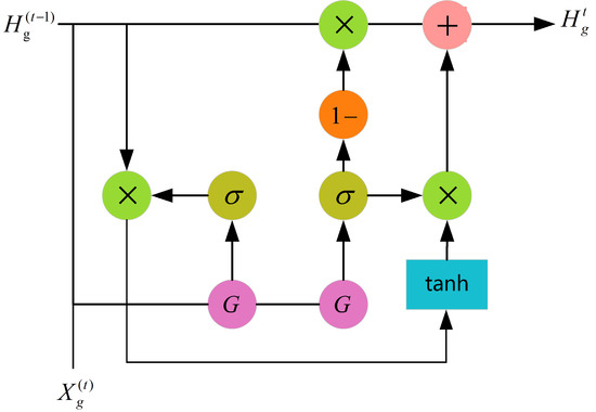
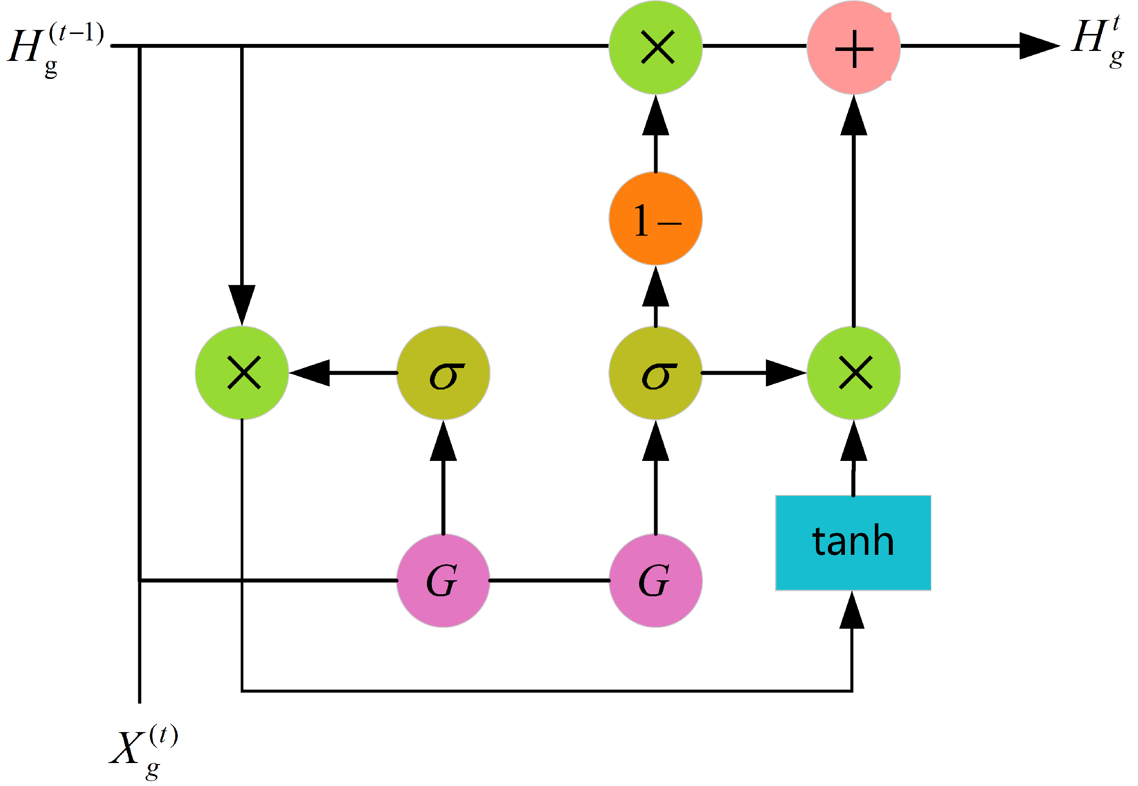
Leveraging the strength of GRUs in modeling local temporal dependencies, we adopt the approach in [51] to integrate GRU with graph convolution, forming the GCGRU module to capture spatiotemporal features of traffic flow. The architecture of this module is illustrated in Figure 5.

Figure 5. The architecture of GCGRU.

The structure of GCGRU is illustrated in Figure 5. Its formulation is as follows.

$$r^{(t)}=\sigma \left({\Theta }_{r\star \mathcal{G}}\left[X_g^{(t)},H^{(t-1)}\right]+b_r\right)$$

(8)

$$u^{(t)}=\sigma \left({\Theta }_{u\star \mathcal{G}}\left[X_g^{(t)},H^{(t-1)}\right]+b_u\right)$$

(9)

$$C^{(t)}=\tanh \left({\Theta }_{C\star \mathcal{G}}\left[X_g^{(t)},r^{(t)}\odot H^{(t-1)}\right]+b_c\right)$$

(10)

$$H_g^{(t)}=u^{(t)}\odot H_g^{(t-1)}+\left(1-u^{(t)}\right)\odot C^{(t)}$$

(11)

Here, $X_g^{(t)}$ and $H_g^{(t)}$ denote the input and output at time step t, respectively; $r(t)$ and $u(t)$ represent the reset and update gates at time t; $\star \mathcal{G}$ denotes the diffusion convolution operation; and ${\mathsf{\Theta }}_r$, ${\mathsf{\Theta }}_u$, and ${\mathsf{\Theta }}_C$ correspond to the associated filter parameters. Similar to standard GRU, this module can be used to construct recurrent neural network layers and trained via backpropagation through time.

In the HCGRU module, temporal feature extraction is conducted similarly to the GCGRU, except that graph convolution is replaced by hypergraph convolution, enabling the capture of higher-order spatiotemporal dependencies among road segments.

3.3.2. Global Temporal Feature Extraction Based on Transformer

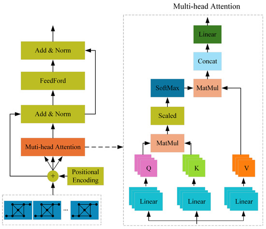
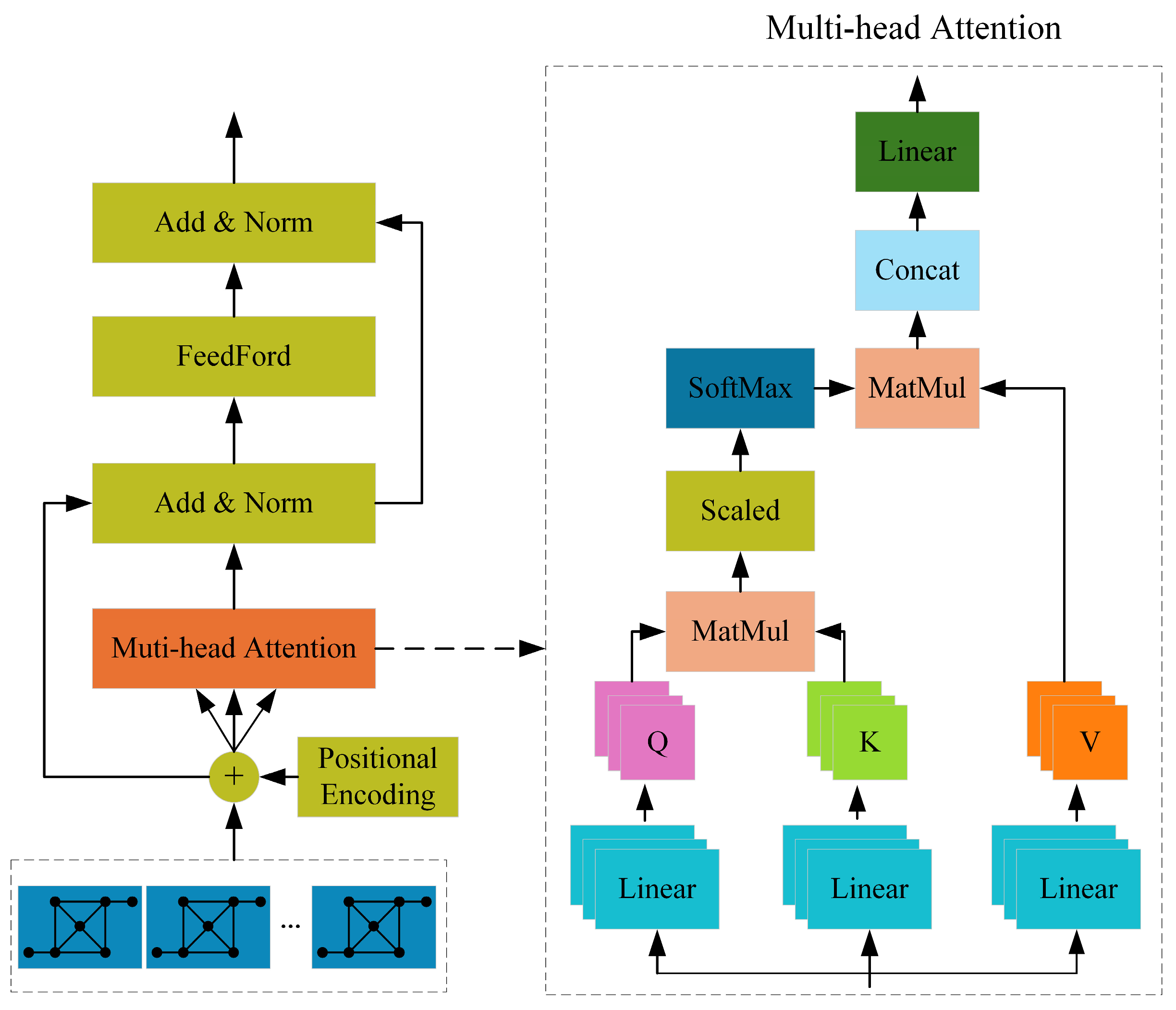
Although GRUs are effective in capturing local temporal dependencies in traffic flow, they exhibit limitations when modeling long-range global dependencies. This is particularly evident when predicting traffic variations across peak periods or under external disturbances, where GRUs are prone to gradient vanishing and information loss. To address this limitation, we introduce a Transformer module following the spatiotemporal fusion module, enabling the extraction of global temporal dynamics from traffic flow sequences. The structure of the Transformer unit and the multi-head attention module is illustrated in Figure 6.

Figure 6. The structure of the Transformer unit and the multi-head attention module.

Specifically, the core of the Transformer lies in the Multi-head Self-Attention (MSA) mechanism, which adaptively assigns attention weights based on the correlations among different time steps, thereby enabling global dependency modeling. For the input sequence X, it is first projected into the query (Q), key (K), and value (V) matrices. The corresponding computation is formulated as follows.

$$\mathrm{Q}=X{\mathrm{W}}_{\mathrm{Q}}$$

(12)

$$K=X{\mathrm{W}}_{\mathrm{K}}$$

(13)

$$\mathrm{V}=X{\mathrm{W}}_V$$

(14)

Here, X denotes the input sequence, while ${\mathrm{W}}_{\mathrm{Q}}$, ${\mathrm{W}}_{\mathrm{K}}$, and ${\mathrm{W}}_{\mathrm{V}}$ are learnable parameters. The attention mechanism captures global dependencies by computing the similarity between any two time steps.

$$\mathrm{Attention}(\mathrm{Q},\mathrm{K},\mathrm{V})=\mathrm{Softmax}\left({\displaystyle \frac{{\mathrm{QK}}^{\top }}{\sqrt{d^{\prime }}}}\right)\mathrm{V}$$

(15)

To improve the modeling of diverse temporal patterns, a multi-head attention mechanism is employed, projecting the input into multiple subspaces and performing parallel computations, as illustrated below.

$$\mathrm{MSA}(\mathrm{Q},\mathrm{K},\mathrm{V})=\mathrm{Concat}\left({\mathrm{head}}_1,\dots ,{\mathrm{head}}_h\right){\mathrm{W}}_{\mathrm{O}}$$

(16)

Here, ${\mathrm{head}}_i=\mathrm{Attention}({\mathrm{QW}}_{\mathrm{Q}}^{\mathrm{i}}{,\mathrm{KW}}_{\mathrm{K}}^{\mathrm{i}}{,\mathrm{VW}}_{\mathrm{V}}^{\mathrm{i}})$, $h$ denotes the number of attention heads, and ${\mathrm{W}}_{\mathrm{O}}$ represents the output projection matrix.

The Multi-head Attention mechanism captures diverse global dependencies from different subspaces, thereby enhancing the representation capacity of traffic flow features. Its key advantage lies in directly modeling the correlations between any two time steps, which alleviates the issue of excessively long dependency paths inherent in recurrent structures. Moreover, to compensate for the lack of temporal positional information in the self-attention mechanism, positional encoding is incorporated during the encoding process to ensure that the model is aware of the sequential order of traffic flow data.

Through these mechanisms, the Transformer is able to effectively model long-range temporal dependencies across different time spans, particularly in forecasting tasks involving cross-day or cross-peak traffic scenarios. It can robustly capture long-term non-stationary variations caused by sudden incidents, demand surges, or road closures. In summary, the Transformer-based global temporal feature extraction not only addresses the limitations of GRUs in long-range dependency modeling but also complements the local temporal feature extraction module.

3.4. Loss Function

In this study, we employ the Mean Absolute Error (MAE) as the loss function during model training, which can be defined as follows.

$${\mathcal{L}}_{\mathrm{MAE}}={\displaystyle \frac{1}{N\ast T}}{\displaystyle \sum _{n=1}^N}{\displaystyle \sum _{t=1}^T}|{\widehat{y}}_n^t-y_n^t|$$

(17)

Here, $N$ and $T$ denote the number of traffic nodes and the length of the prediction time horizon, respectively, while ${\widehat{y}}_n^t$ and $y_n^t$ represent the predicted and ground-truth traffic flow values for the n-th node at the t-th time step.

4. Experiments

4.1. Experimental Settings

4.1.1. Dataset Description and Preprocessing

In this study, we evaluate the proposed HSTGHN model on six publicly available traffic network datasets, namely METR-LA, PEMS-BAY, PEMS03, PEMS04, and PEMS08. METR-LA and PEMS-BAY contain traffic speed measurements collected from freeway sensor networks in Los Angeles County and the Bay Area, respectively. In contrast, PEMS03, PEMS04, and PEMS08 originate from the Caltrans Performance Measurement System (PEMS) and provide traffic flow measurements from different highway districts in California. Together, these datasets cover diverse spatial network structures and temporal traffic patterns, offering a comprehensive benchmark for evaluating the generalization ability of the proposed model. A detailed description of the datasets is provided in Table 1.

Table 1. Dataset descriptions.

Dataset	Nodes	Edges	Time Steps	Predicted Value
METR-LA	207	1515	34,272	speed
PEMS-BAY	325	2369	52,116	speed
PEMS03	358	547	26,208	flow
PEMS04	307	340	16,992	flow
PEMS08	170	295	17,856	flow

Following the data preprocessing procedure outlined in [23], sensor readings are first aggregated into 5-min intervals. Missing values are handled through temporal interpolation, and outliers are filtered using established traffic data cleaning rules. Subsequently, node adjacency matrices are constructed using a Gaussian kernel based on road network distances and a predefined threshold. All input features are normalized using the Z-score standardization method to ensure consistent value ranges across different sensors and improve model training stability, as shown in Equation (18). Finally, each dataset is chronologically divided into 70% for training, 10% for validation, and 20% for testing, ensuring strict temporal consistency and preventing information leakage between sets.

$$x_{i,t}^{norm}={\displaystyle \frac{x_{i,t}-{\mu }_i}{{\sigma }_i}}$$

(18)

Here, $x_{i,t}$ denotes the original traffic flow (or speed) value of sensor $i$ at time $t$, ${\mu }_i$ is the historical mean of sensor $i$, ${\sigma }_i$ is the historical standard deviation of sensor $i$.

4.1.2. Baselines

To evaluate the effectiveness and superiority of the proposed HSTGHN model in traffic flow forecasting, a set of representative baseline models was selected for comparative experiments from multiple perspectives. These baselines cover models that consider only temporal dependencies, spatiotemporal forecasting models based on static road networks, and graph neural network models capable of capturing dynamic spatial dependencies. Such a comprehensive selection allows for a hierarchical performance evaluation, ranging from purely temporal modeling, through static spatiotemporal fusion, to dynamic spatiotemporal dependency modeling.

Models considering only temporal dependencies:

• ARIMA [43]: A classical statistical learning model that captures linear temporal dependencies using autoregressive and moving average components. While effective for linear sequences, ARIMA struggles with the nonlinear and multi-scale variations typical of traffic flows.
• LSTM [52]: Long Short-Term Memory networks incorporate input, forget, and output gates to mitigate the gradient vanishing problem in traditional RNNs. LSTM excels at capturing long-range temporal dependencies.
• GRU [10]: Gated Recurrent Units are structurally simpler than LSTMs, containing only update and reset gates, which reduces the number of parameters while maintaining high predictive accuracy and computational efficiency.

Static spatiotemporal graph neural network models:

• DCRNN [23]: Diffusion Convolutional Recurrent Neural Networks introduce diffusion convolutions on directed weighted graphs to simulate traffic flow propagation, combined with sequence-to-sequence RNNs for temporal modeling.
• ASTGCN [15]: Attention-based Spatiotemporal Graph Convolutional Networks employ temporal attention, spatial attention, and spatiotemporal convolution modules to dynamically adjust the importance of different time slices and nodes.
• Graph WaveNet [37]: Graph WaveNet integrates first-order graph convolution with an adaptive adjacency matrix learning mechanism, leveraging dilated convolutions for multi-scale temporal modeling and capable of learning latent spatial connections without prior knowledge of the road network.
• DDSTGCN [33]: Dual Dynamic Spatiotemporal Graph Convolutional Networks combine static adjacency matrices with adaptive dynamic graphs to enhance spatial correlation modeling flexibility, and incorporate multi-scale convolutions along the temporal dimension.

Dynamic spatiotemporal graph neural network models:

• D2STGNN [53]: Dual Dynamic Spatiotemporal Graph Neural Networks introduce dynamic graph construction mechanisms along both spatial and temporal dimensions, allowing the model to adapt to time-varying traffic network structures.
• MegaCRN [42]: Memory-augmented Graph Convolutional Recurrent Networks capture long-term global patterns via memory units while learning dynamic adjacency matrices, balancing historical dependencies with real-time response to traffic perturbations.

By comparing across these diverse baseline models, the performance of HSTGHN can be assessed under varying prediction difficulty levels, and its advantages in modeling complex dynamic spatiotemporal dependencies can be effectively demonstrated.

4.1.3. Evaluation Metrics

To comprehensively evaluate the predictive accuracy of the proposed HSTGHN model, we adopt Mean Absolute Error (MAE), Mean Absolute Percentage Error (MAPE), and Root Mean Square Error (RMSE) as the evaluation metrics, denoted as ${\epsilon }_{\mathrm{MAE}}$ ${\epsilon }_{\mathrm{MAPE}}$ and ${\epsilon }_{\mathrm{RMAE}}$, respectively, and their definitions are as follows.

$${\mathcal{E}}_{\mathrm{MAE}}={\displaystyle \frac{1}{T\cdot N}}{\displaystyle \sum _{t=1}^T{\displaystyle \sum _{n=1}^N\left|{\widehat{y}}_n^t-y_n^t\right|}}$$

(19)

$${\mathcal{E}}_{\mathrm{MAPE}}={\displaystyle \frac{100\%}{T\cdot N}}{\displaystyle \sum _{t=1}^T{\displaystyle \sum _{n=1}^N\left|\frac{{\widehat{y}}_n^t-y_n^t}{{\widehat{y}}_n^t}\right|}}$$

(20)

$${\mathcal{E}}_{\mathrm{RMSE}}=\sqrt{{\displaystyle \frac{1}{T\cdot N}}{\displaystyle \sum _{t=1}^T{\displaystyle \sum _{n=1}^N{\left({\widehat{y}}_n^t-y_n^t\right)}^2}}}$$

(21)

4.1.4. Experimental Environment and Hyperparameter Settings

The experiments were conducted on a system equipped with an AMD Ryzen 7 9800X3D CPU (4.70 GHz) and an NVIDIA GeForce RTX 5070 Ti GPU. The software environment was Windows 11, and the proposed model was implemented using PyTorch 2.7.1.

To determine the optimal hyperparameters for each dataset, we employed Bayesian optimization, which efficiently explores the hyperparameter space to identify configurations that maximize model performance. As shown in Table 2, the optimal hyperparameters for the METR-LA dataset comprise training hyperparameters and sensitivity analysis hyperparameters. It should be noted that similar optimization procedures were conducted for other datasets to obtain their respective optimal hyperparameter configurations.

Table 2. Optimal hyperparameters for the proposed model on METR-LA dataset.

Category	Hyperparameters	Values
Training Hyperparameters	Epoch	200
	Dropout	0.3
	Optimizer	Adam
	Learning rate	0.001
	Decay rate	0.97
Sensitivity Analysis Hyperparameters	hidden layer dimensions.	64
	Number of Top-k.	4
	Number of Attention Heads.	6

4.2. Comparative Analysis of Results

We compare the proposed HSTGHN model with classical time series models and graph neural network-based models in terms of predictive performance across different datasets and forecasting horizons.

As shown in Table 3, the proposed HSTGHN model consistently outperforms all baseline methods across both the METR-LA and PEMS-BAY datasets, demonstrating strong stability and adaptability for traffic speed prediction tasks. Specifically, on the METR-LA dataset, HSTGHN achieves MAE, MAPE, and RMSE values of 2.67/3.05/3.49, 6.77/8.18/9.90%, and 5.09/6.06/7.13, respectively, representing substantial improvements over the second-best model, MegaCRN. On the PEMS-BAY dataset, HSTGHN attains even more impressive results with MAE, MAPE, and RMSE of 1.30/1.62/1.93, 2.71/3.64/4.57%, and 2.73/3.66/4.45, respectively. Compared with the second-best models across both datasets, HSTGHN achieves average improvements of 3.9% in MAE, 7.4% in MAPE, and 2.9% in RMSE. From an interpretability perspective, the superior performance can be attributed to several key architectural innovations. The hierarchical spatiotemporal design enables the model to effectively capture multi-scale dependencies in speed patterns, from local road segment correlations to city-wide propagation dynamics. More importantly, the adaptive graph learning mechanism discovers hidden spatial relationships that traditional distance-based methods may overlook, which is particularly crucial for speed prediction as traffic congestion often propagates through non-obvious pathways. Additionally, the temporal attention component dynamically weights historical information, prioritizing recent speed variations during rush hours while leveraging periodic patterns during regular traffic conditions. The particularly strong performance on PEMS-BAY suggests that HSTGHN is especially effective in capturing the spatiotemporal characteristics of highway networks with relatively stable traffic patterns, where the model’s ability to learn long-range dependencies and implicit spatial correlations provides significant advantages.

Table 3. Comparison of Prediction Results on the METR-LA and PEMS-BAY Datasets.

Dataset	Models	MAE Horizon @3/6/12	MAPE(%) Horizon @3/6/12	RMSE Horizon @3/6/12
Metr-La	ARIMA	3.36/4.07/5.21	9.04/11.59/15.43	6.39/7.84/9.84
	LSTM	3.09/3.79/4.88	8.20/10.64/14.72	6.09/7.64/9.56
	GRU	3.04/3.67/4.59	8.18/10.57/13.24	5.97/7.38/9.11
	DCRNN	2.86/3.27/3.82	7.40/8.94/10.81	5.32/6.38/7.60
	ASTGCN	2.98/3.47/4.15	7.95/9.81/12.31	5.70/6.87/8.29
	GraphWaveNet	2.84/3.25/3.80	7.43/9.10/11.18	5.29/6.38/7.59
	DDSTGCN	2.74/3.16/3.66	7.42/9.01/11.16	5.21/6.25/7.45
	D2STGNN	2.75/3.14/3.63	6.90/8.47/10.29	5.24/6.26/7.39
	MegaCRN	2.73/3.12/3.58	7.32/8.90/10.72	5.13/6.18/7.26
	HSTGHN(ours)	2.67/3.05/3.49	6.77/8.18/9.90	5.09/6.06/7.13
Pems-Bay	ARIMA	1.64/2.16/2.89	3.48/4.84/6.98	3.53/4.95/6.52
	LSTM	1.55/2.04/2.78	3.19/4.47/6.60	3.35/4.79/6.41
	GRU	1.45/1.91/2.53	3.06/4.37/6.39	3.07/4.33/5.78
	DCRNN	1.41/1.85/2.40	2.94/4.23/6.03	3.04/4.28/5.54
	ASTGCN	1.71/1.92/2.40	4.14/4.60/5.95	3.72/4.26/5.41
	GraphWaveNet	1.54/2.04/2.77	3.19/4.47/6.60	3.35/4.79/6.41
	DDSTGCN	1.42/1.74/2.06	3.19/4.03/4.89	2.92/3.81/4.60
	D2STGNN	1.40/1.72/2.06	3.12/4.02/4.91	2.92/3.84/4.62
	MegaCRN	1.36/1.71/2.07	2.88/3.90/4.97	2.86/3.81/4.69
	HSTGHN(ours)	1.30/1.62/1.93	2.71/3.64/4.57	2.73/3.66/4.45

Table 4 presents comprehensive experimental results on traffic flow prediction across three datasets with varying scales and characteristics. HSTGHN achieves MAE, MAPE, and RMSE of 13.68/14.97/17.06, 14.12/15.05/16.57%, and 22.00/24.55/28.20 on PEMS03, and 18.55/19.78/21.94, 13.08/13.88/15.41%, and 29.61/31.35/34.16 on PEMS04. The most remarkable improvements are observed on PEMS08, where HSTGHN achieves 14.30/15.53/17.64, 9.72/10.54/11.99%, and 22.46/24.53/27.61, with average improvements of 2.4% in MAE, 6.0% in MAPE, and 3.2% in RMSE across all datasets. These exceptional results can be attributed to the model’s hierarchical decomposition strategy, which effectively captures flow dynamics at multiple granularities. Unlike speed prediction, flow forecasting requires modeling simultaneous accumulation and dispersion dynamics at intersections, which HSTGHN addresses through adaptive graph learning that identifies critical transfer relationships beyond physical road connectivity. The superior performance on PEMS08, with its diverse sensor types and complex topology, demonstrates the model’s robustness in handling heterogeneous traffic scenarios. Furthermore, the integrated gating mechanisms provide implicit noise filtering while retaining informative temporal patterns, enabling HSTGHN to generalize effectively across datasets with fundamentally different characteristics and network complexities.

Table 4. Comparison of Traffic Flow Prediction Results on the PEMS03, PEMS04, and PEMS08 Datasets.

Dataset	Models	MAE Horizon @3/6/12	MAPE(%) Horizon @3/6/12	RMSE Horizon @3/6/12
PEMS03	ARIMA	21.44/25.33/33.06	68.76/72.78/85.84	33.02/38.93/50.59
	LSTM	18.64/22.23/36.17	16.68/21.85/39.78	25.11/29.07/43.72
	GRU	17.10/20.13/26.65	25.40/27.32/35.28	28.35/32.90/42.01
	DCRNN	16.64/19.91/27.18	17.70/19.91/27.18	27.58/32.39/43.23
	ASTGCN	19.02/18.75/21.82	24.89/24.03/28.94	31.66/31.70/36.27
	GraphWaveNet	13.73/15.09/17.61	14.57/15.37/17.44	23.53/25.95/29.66
	DDSTGCN	13.91/15.20/17.32	14.65/15.54/16.65	24.25/26.18/29.11
	D2STGNN	14.03/15.28/17.52	14.42/16.23/19.64	24.26/26.38/29.25
	MegaCRN	14.03/15.32/17.32	18.32/19.26/20.09	23.94/25.96/28.91
	HSTGHN(ours)	13.68/14.97/17.06	14.12/15.05/16.57	22.00/24.55/28.20
PEMS04	ARIMA	25.16/30.88/50.15	20.43/23.14/42.92	35.27/41.66/62.16
	LSTM	22.24/26.21/35.05	29.21/31.98/38.46	34.96/40.51/52.24
	GRU	22.15/26.09/34.83	28.06/30.79/37.44	34.54/40.01/51.76
	DCRNN	21.27/24.63/32.06	17.79/19.76/25.28	32.98/37.54/47.37
	ASTGCN	22.96/22.49/26.30	19.12/18.31/21.04	36.32/35.99/41.82
	GraphWaveNet	20.01/21.90/25.39	14.31/15.10/17.20	31.30/34.01/38.70
	DDSTGCN	18.86/20.35/22.73	13.16/14.11/15.76	29.93/32.07/35.24
	D2STGNN	19.26/20.97/23.82	14.59/16.57/18.52	30.34/32.61/36.45
	MegaCRN	19.11/20.76/23.62	13.57/14.56/16.45	30.19/32.42/36.23
	HSTGHN(ours)	18.55/19.78/21.94	13.08/13.88/15.41	29.61/31.35/34.16
PEMS08	ARIMA	26.35/30.45/39.49	16.25/27.39/42.19	50.08/62.04/75.88
	LSTM	17.80/21.22/29.02	30.62/32.52/39.90	27.67/33.03/43.77
	GRU	17.58/20.90/28.48	19.03/21.37/27.54	29.08/34.14/42.58
	DCRNN	16.14/18.25/22.83	12.05/13.25/16.76	24.79/28.17/34.64
	ASTGCN	19.26/19.69/23.75	15.98/15.86/19.49	28.29/29.45/35.22
	GraphWaveNet	16.30/17.70/20.36	11.46/12.41/15.13	25.04/27.40/31.27
	DDSTGCN	14.88/16.24/18.94	11.35/12.10/13.75	23.05/25.29/29.21
	D2STGNN	14.70/16.01/18.35	11.90/12.35/13.36	22.80/25.05/28.45
	MegaCRN	14.62/16.22/18.99	11.16/12.18/13.24	22.97/25.62/29.55
	HSTGHN(ours)	14.30/15.53/17.64	9.72/10.54/11.99	22.46/24.53/27.61

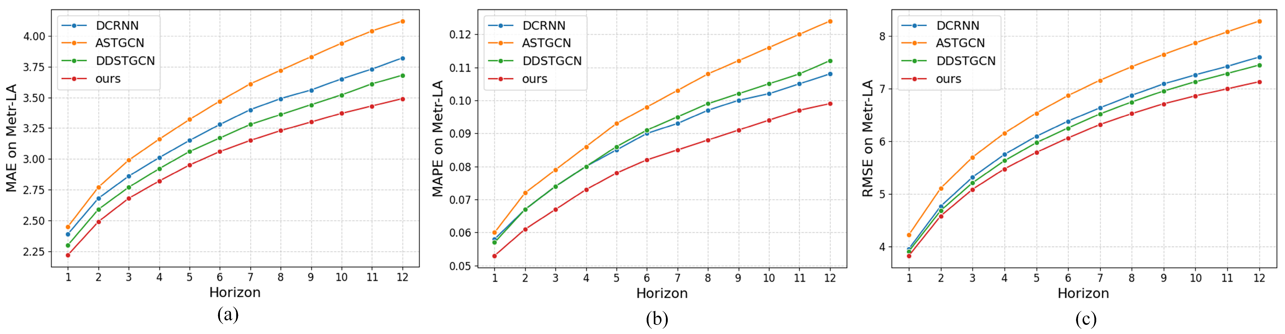
As shown in Figure 7, the evaluation metrics of DCRNN, ASTGCN, DDSTGCN, and our model on the METR-LA dataset demonstrate that our approach achieves superior performance across both short- and long-term horizons. This advantage can be attributed to three aspects. First, in terms of model architecture, graph-based methods generally outperform pure temporal models by incorporating structural information among road nodes; however, models such as DCRNN use undirected graphs that overlook bidirectional connectivity, while DDSTGCN relies on adaptive adjacency matrices but lacks prior knowledge of road topology. Second, with respect to prediction horizon, our model achieves significantly higher accuracy at 12-step (1-h) forecasting due to the Transformer’s strength in modeling long-range temporal dependencies. Third, regarding dataset characteristics, the large-scale PEMS-BAY dataset with complex adjacency relationships highlights the robustness of our framework, as the integration of an HGCN-based edge feature extraction module enables more effective representation of structural information compared with competing methods.

Figure 7. Comparison of Evaluation Metrics on the METR-LA Dataset. (a) MAE. (b) MAPE. (c) RMSE.

4.3. Ablation Studies

To systematically evaluate the contribution of each component, we conducted ablation studies with the following settings:

• w/o HGCN: replacing the hypergraph convolution in the HCGRU module with a standard graph convolution.
• w/o $A_{adp}$: removing the adaptive adjacency matrix in the GCGRU module and using only the static prior adjacency matrix.
• w/o GRU: the GRU module in HCGRU and GCGRU is removed and replaced with a linear layer.
• w/o Transformer: discarding the Transformer module in the temporal modeling part and substituting it with a linear layer.

The complete HSTGHN model is compared against these w/o versions to validate the effectiveness of each component.

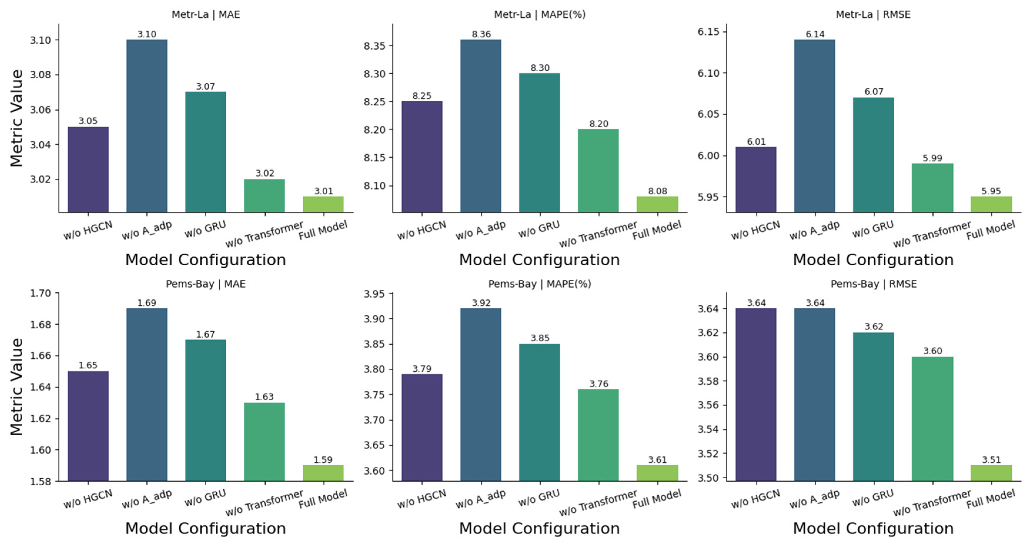
To validate the effectiveness of each component in our proposed model, we conducted comprehensive ablation studies on the METR-LA and PEMS-BAY datasets, as shown in Table 5. The complete model, incorporating all four components (HGCN, A_adp, GRU, and Transformer), achieved the best performance. The ablation experiments highlight the distinct contributions of each component. Removing the Transformer caused the performance drop, emphasizing its role in capturing long-range temporal dependencies. Excluding the GRU led to notable decline, showing the importance of modeling short-term sequential patterns. The absence of the adaptive adjacency matrix moderately reduced accuracy, indicating its value in learning latent spatial relationships. Removing HGCN also degraded performance, confirming its role in extracting multi-scale spatial features. Overall, these results demonstrate that each component contributes uniquely, and their combined integration significantly enhances prediction accuracy across datasets.

Table 5. Ablation Study Results on the METR-LA and PEMS-BAY Datasets.

		Components		Dataset
HGCN	${\mathit{A}}_{\mathit{a}\mathit{d}\mathit{p}}$	GRU	Transformer	METR-LA			PEMS-BAY
				MAE	MAPE(%)	RMSE	MAE	MAPE(%)	RMSE
	✓	✓	✓	3.05	8.25	6.01	1.65	3.79	3.64
✓		✓	✓	3.10	8.36	6.14	1.69	3.92	3.64
✓	✓		✓	3.07	8.30	6.07	1.67	3.85	3.62
✓	✓	✓		3.02	8.20	5.99	1.63	3.76	3.60
✓	✓	✓	✓	3.01	8.08	5.95	1.59	3.61	3.51

The performance comparison across different component configurations is visualized in Figure 8. The bar charts show that across all three evaluation metrics on both datasets, the full HSTGHN configuration (HGCN + A_adp + GRU + Transformer) consistently outperforms all ablated variants. This visualization highlights the cumulative benefits of integrating all four modules, with each component contributing to the overall improvement. Notably, configurations including either GRU or Transformer achieve intermediate performance, while adding the adaptive adjacency matrix further enhances prediction accuracy. The combination of HGCN and GRU captures essential spatiotemporal patterns, and the inclusion of the Transformer can provide additional temporal context. These results reinforce the quantitative findings from Table 5, demonstrating that the superior performance of HSTGHN arises from the synergistic effect of all architectural components.

Figure 8. Visualization of model evaluation metrics under different model configurations.

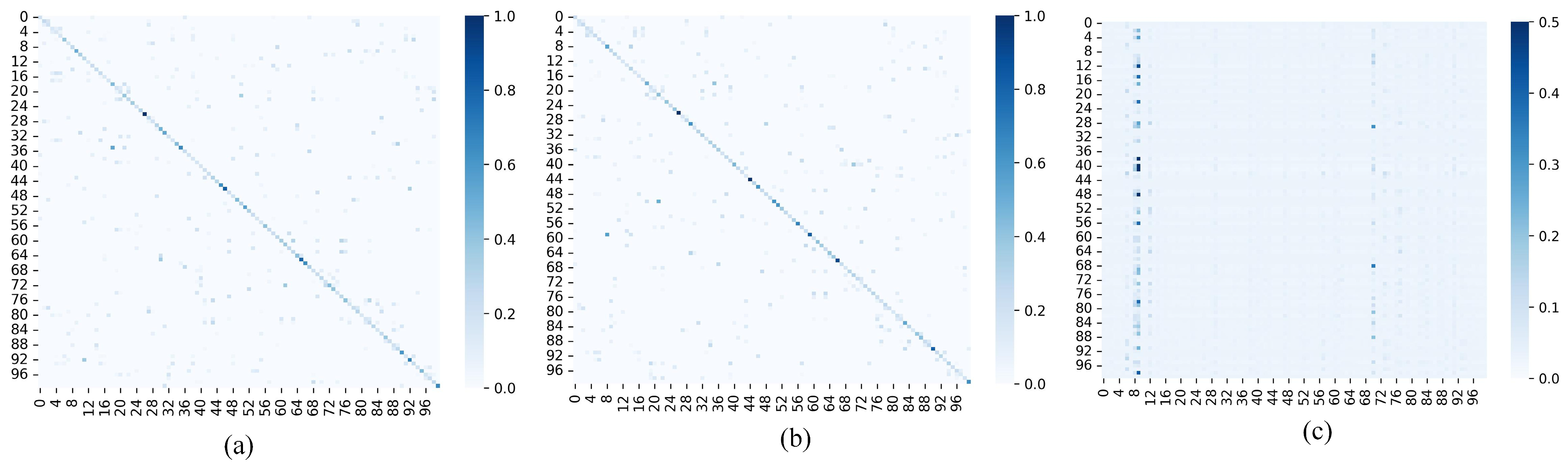
We further visualized the learned graph adjacency matrices, as shown in Figure 9. Here, $X_f$ and $X_b$ represent the forward and backward relationships, respectively, while $X_{adp}$ denotes the adaptive adjacency matrix learned from data. It can be observed that the adaptive adjacency matrix compensates for the limitations of the static graphs by capturing the latent dependencies between nodes.

Figure 9. Visualization of graph adjacency matrices. (a) Forward adjacency matrix. (b) Backward adjacency matrix. (c) Adaptive adjacency matrix.

4.4. Sensitivity Analysis of Hyperparameters

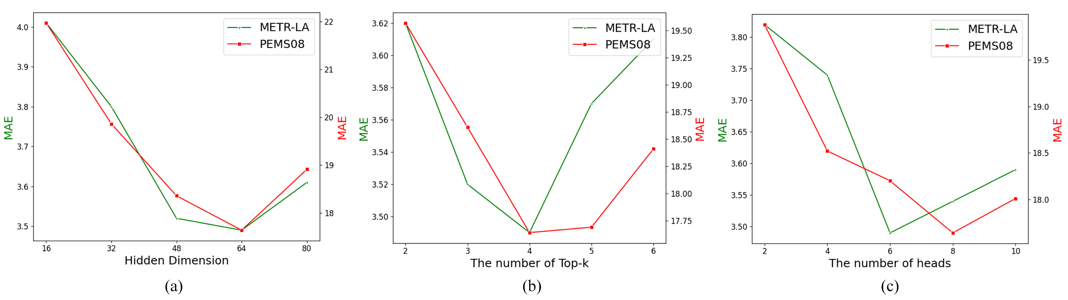
To evaluate the sensitivity of the proposed HSTGHN model to key hyperparameters, we conducted experiments on the METR-LA and PEMS08 datasets using MAE as the evaluation metric. The analysis primarily focused on three hyperparameters: the hidden layer dimension of the model, the number of hypernodes selected by the Top-k parameter in the HGCN module, and the number of attention heads in the Transformer module. The experimental results are presented in Figure 10.

Figure 10. Comparison under Different Hyperparameter Settings on the METR-LA and PEMS08 Datasets. (a) MAE under different numbers of hidden layer dimensions. (b) MAE under different values of Top-k. (c) MAE under different numbers of heads.

Hidden Layer Dimension. The hidden dimension determines the number of feature channels for graph and hypergraph nodes (or hypernodes), i.e., the number of intermediate filters. As the hidden dimension increases, the model’s representation capacity is enhanced, leading to improved prediction accuracy. However, when the dimension exceeds a certain threshold, the model complexity grows substantially, which may result in overfitting and cause the performance to plateau or slightly degrade. Experimental results indicate that setting the hidden dimension to 64 achieves the best trade-off between expressive power and generalization.

Top-k Parameter. The Top-k parameter in the HGCN module controls the number of hypernodes, thereby affecting the complexity and expressive capacity of the hypergraph. Results show that moderately increasing k improves model performance, while excessively large values introduce noise and redundant information, leading to performance degradation. The experiments demonstrate that the optimal performance on both datasets is obtained when k = 4.

Number of Attention Heads. The number of attention heads in the Transformer module governs the model’s ability to capture diverse temporal dependency patterns. The results reveal that the optimal setting is achieved with 6 heads on the METR-LA dataset and 8 heads on the PEMS08 dataset. This suggests that an appropriate number of attention heads enables the model to better capture the complex temporal dependencies inherent in traffic data, whereas an excessively large number may lead to overfitting and reduced performance.

4.5. Visualization of Experimental Results

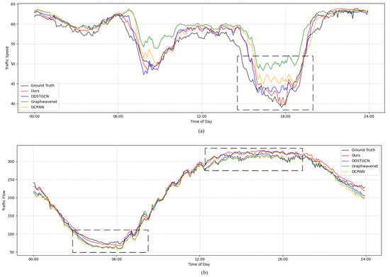
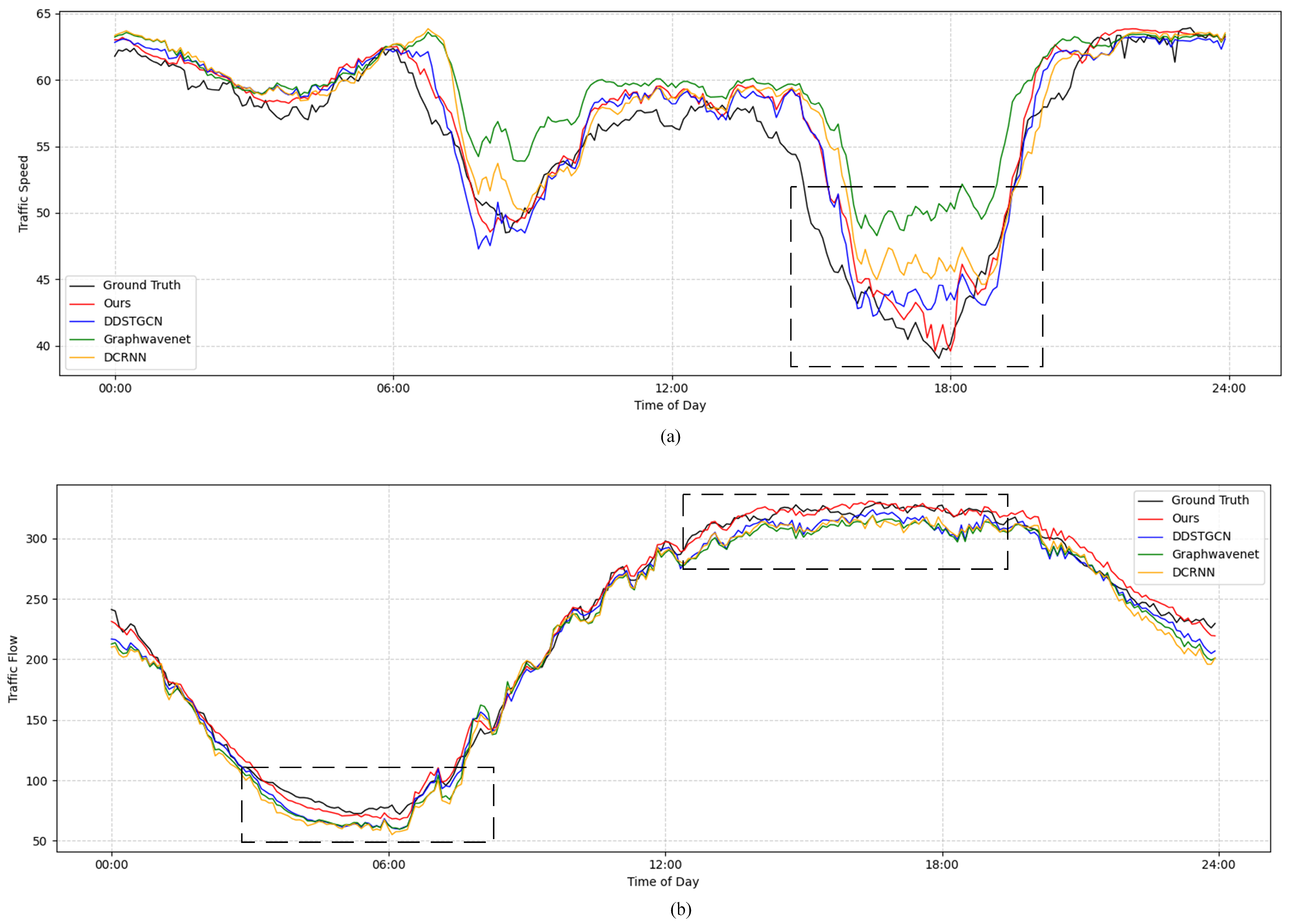
To intuitively demonstrate the performance of the proposed model, we conducted a visualization analysis of the prediction results on two public traffic datasets. For the METR-LA dataset, we focused on speed prediction, whereas for the PEMS08 dataset, we visualized traffic flow predictions. To capture overall trends, the predictions were averaged across all nodes at each time step throughout the day and compared with the corresponding ground-truth observations. Figure 11 illustrates the predictive performance of different models on these two datasets, providing a clear visualization of the proposed model’s capability in capturing traffic dynamics.

Figure 11. Model Prediction Results on the METR-LA and PEMS08 Datasets. (a) Comparison of speed prediction results of different models on the METR-LA dataset. (b) Comparison of traffic flow prediction results of different models on the PEMS08 dataset.

The visualization results indicate that our model achieves high predictive accuracy across critical time periods. In the speed prediction task on the METR-LA dataset, the model notably captures the speed variations during the afternoon peak hours (17:00–19:00), outperforming baseline models. Similarly, in the traffic flow prediction task on the PEMS08 dataset, the model demonstrates superior performance during both the early morning free-flow period (05:00–07:00) and the afternoon congestion peak, with predicted traffic volumes closely aligning with observed values. These results demonstrate that the proposed model possesses superior capability in capturing spatiotemporal representations and exhibits strong generalization across diverse traffic scenarios.

5. Conclusions

In this study, we propose the HSTGHN model to address the challenges of spatiotemporal modeling in traffic flow prediction and to support the development of more efficient and sustainable urban mobility systems. The model incorporates a Hypergraph Convolutional Network (HGCN) to capture high-order spatial dependencies among road segments, while a data-driven adaptive adjacency matrix dynamically represents evolving correlations within the transportation network. For spatiotemporal feature extraction, HCGRU and GCGRU modules effectively learn short-term traffic dynamics, and a Transformer module captures long-term temporal dependencies, with their complementary strengths significantly improving predictive performance. Moreover, the integration of graph and hypergraph convolutions enriches the spatial representation and enhances model robustness in complex traffic environments. Extensive experiments on six real-world datasets show that HSTGHN consistently outperforms state-of-the-art methods in predictive accuracy and stability, particularly in long-term forecasting and highly dynamic traffic scenarios. Although the Transformer component increases model complexity, future work will explore more lightweight and energy-efficient spatiotemporal architectures to further balance forecasting accuracy, computational efficiency, and the sustainability requirements of large-scale intelligent transportation systems.

6. Limitations and Future Work

Although HSTGHN achieves competitive predictive performance, several limitations merit attention. The study relies on PEMS and METR-LA datasets, which capture only single-modality traffic flows without complementary contextual factors such as weather events or temporal patterns. This geographic limitation may affect model transferability across diverse urban environments—a critical consideration for sustainable smart city deployments.

Computational demands remain substantial due to hypergraph construction and Transformer operations, potentially hindering scalability for resource-constrained municipalities pursuing sustainable transportation management. Future work will explore lightweight architectures, including sparse hypergraph formulations and efficient attention mechanisms, to enable broader adoption in cities with limited computational infrastructure.

Additionally, robustness to sensor failures, data gaps, and sudden distribution shifts remains unexplored. Expanding evaluations to multimodal datasets, testing across varied geographic contexts, and investigating adaptive learning mechanisms represent valuable directions. These efforts align with sustainable development goals by promoting resilient, equitable urban transportation systems that can adapt to evolving environmental and societal needs.

References

- Kumar, R.; Bhanu, M.; Mendes-Moreira, J.; Chandra, J. Spatio-temporal predictive modeling techniques for different domains: A survey. ACM Comput. Surv. 2024, 57, 1–42. [Google Scholar] [CrossRef] [Scilit]
- Yang, H.; Yao, X.A.; Roozkhosh, F.; Liu, R.; Mai, G. From theory to deep learning: Understanding the impact of geographic context factors on traffic violations. Comput. Environ. Urban Syst. 2025, 119, 102268. [Google Scholar] [CrossRef] [Scilit]
- Zhang, L.; Li, S.; Liu, Y.; Huang, H.; Van de Weghe, N. From grids to dendrites: Quantifying spatial heterogeneity in urban road networks. Comput. Environ. Urban Syst. 2025, 121, 102309. [Google Scholar] [CrossRef] [Scilit]
- Klepsch, J.; Klüppelberg, C.; Wei, T. Prediction of functional ARMA processes with an application to traffic data. Econ. Stat. 2017, 1, 128–149. [Google Scholar] [CrossRef] [Scilit]
- Tian, M.; Sun, C.; Wu, S. An EMD and ARMA-based network traffic prediction approach in SDN-based internet of vehicles. Wirel. Netw. 2021, 1–13. [Google Scholar] [CrossRef] [Scilit]
- Yuan, C.; Yu, X.; Li, D.; Xi, Y. Overall traffic mode prediction by VOMM approach and AR mining algorithm with large-scale data. IEEE Trans. Intell. Transp. Syst. 2018, 20, 1508–1516. [Google Scholar] [CrossRef] [Scilit]
- Chen, R.; Liang, C.-Y.; Hong, W.-C.; Gu, D.-X. Forecasting holiday daily tourist flow based on seasonal support vector regression with adaptive genetic algorithm. Appl. Soft Comput. 2015, 26, 435–443. [Google Scholar] [CrossRef] [Scilit]
- Hou, Y.; Edara, P.; Sun, C. Traffic flow forecasting for urban work zones. IEEE Trans. Intell. Transp. Syst. 2014, 16, 1761–1770. [Google Scholar] [CrossRef] [Scilit]
- Huang, W.; Song, G.; Hong, H.; Xie, K. Deep architecture for traffic flow prediction: Deep belief networks with multitask learning. IEEE Trans. Intell. Transp. Syst. 2014, 15, 2191–2201. [Google Scholar] [CrossRef] [Scilit]
- Cho, K.; van Merrienboer, B.; Gulcehre, C.; Bougares, F.; Schwenk, H.; Bengio, Y. Learning phrase representations using RNN encoder-decoder for statistical machine translation. In Proceedings of the Conference on Empirical Methods in Natural Language Processing (EMNLP 2014), Doha, Qatar, 26–28 October 2014. [Google Scholar]
- Lea, C.; Flynn, M.D.; Vidal, R.; Reiter, A.; Hager, G.D. Temporal convolutional networks for action segmentation and detection. In Proceedings of the IEEE Conference on Computer Vision and Pattern Recognition, Honolulu, HI, USA, 21–26 July 2017; pp. 156–165. [Google Scholar]
- Fafoutellis, P.; Vlahogianni, E.I. A theory-informed multivariate causal framework for trustworthy short-term urban traffic forecasting. Transp. Res. Part C Emerg. Technol. 2025, 170, 104945. [Google Scholar] [CrossRef] [Scilit]
- Wu, X.; Chow, A.H.; Ma, W.; Lam, W.H.; Wong, S.C. Prediction of traffic state variability with an integrated model-based and data-driven Bayesian framework. Transp. Res. Part C Emerg. Technol. 2025, 171, 104953. [Google Scholar] [CrossRef] [Scilit]
- Chen, J.; Ye, H.; Ying, Z.; Sun, Y.; Xu, W. Dynamic trend fusion module for traffic flow prediction. Appl. Soft Comput. 2025, 174, 112979. [Google Scholar] [CrossRef] [Scilit]
- Guo, S.; Lin, Y.; Feng, N.; Song, C.; Wan, H. Attention based spatial-temporal graph convolutional networks for traffic flow forecasting. In Proceedings of the AAAI Conference on Artificial Intelligence, Honolulu, HI, USA, 27 January–1 February 2019; pp. 922–929. [Google Scholar]
- Kipf, T. Semi-Supervised Classification with Graph Convolutional Networks. arXiv 2016, arXiv:1609.02907. [Google Scholar]
- Ta, X.; Liu, Z.; Hu, X.; Yu, L.; Sun, L.; Du, B. Adaptive spatio-temporal graph neural network for traffic forecasting. Knowl.-Based Syst. 2022, 242, 108199. [Google Scholar] [CrossRef] [Scilit]
- Li, Z.; Zhou, J.; Lin, Z.; Zhou, T. Dynamic spatial aware graph transformer for spatiotemporal traffic flow forecasting. Knowl.-Based Syst. 2024, 297, 111946. [Google Scholar] [CrossRef] [Scilit]
- Liu, A.; Zhang, Y. Spatial–temporal dynamic graph convolutional network with interactive learning for traffic forecasting. IEEE Trans. Intell. Transp. Syst. 2024, 25, 7645–7660. [Google Scholar] [CrossRef] [Scilit]
- Bruna, J.; Zaremba, W.; Szlam, A.; LeCun, Y. Spectral networks and deep locally connected networks on graphs. In Proceedings of the 2nd International Conference on Learning Representations, ICLR 2014, Banff, AB, Canada, 14–16 April 2014. [Google Scholar]
- Defferrard, M.; Bresson, X.; Vandergheynst, P. Convolutional neural networks on graphs with fast localized spectral filtering. Adv. Neural Inf. Process. Syst. 2016, 29, 3844–3852. [Google Scholar]
- Hamilton, W.; Ying, Z.; Leskovec, J. Inductive representation learning on large graphs. Adv. Neural Inf. Process. Syst. 2017, 30, 1024–1034. [Google Scholar]
- Li, Y.; Yu, R.; Shahabi, C.; Liu, Y. Diffusion Convolutional Recurrent Neural Network: Data-Driven Traffic Forecasting. In Proceedings of the International Conference on Learning Representations, Vancouver, BC, Canada, 30 April–3 May 2018. [Google Scholar]
- Zhang, W.; Zhu, F.; Lv, Y.; Tan, C.; Liu, W.; Zhang, X.; Wang, F.-Y. AdapGL: An adaptive graph learning algorithm for traffic prediction based on spatiotemporal neural networks. Transp. Res. Part C Emerg. Technol. 2022, 139, 103659. [Google Scholar] [CrossRef] [Scilit]
- Bai, S.; Zhang, F.; Torr, P.H. Hypergraph convolution and hypergraph attention. Pattern Recognit. 2021, 110, 107637. [Google Scholar] [CrossRef] [Scilit]
- Antelmi, A.; Cordasco, G.; Polato, M.; Scarano, V.; Spagnuolo, C.; Yang, D. A survey on hypergraph representation learning. ACM Comput. Surv. 2023, 56, 1–38. [Google Scholar] [CrossRef] [Scilit]
- Wang, K.; Shen, Z.; Lei, Z.; Liu, X.; Zhang, T. Towards multi-agent reinforcement learning based traffic signal control through spatio-temporal hypergraphs. IEEE Trans. Mob. Comput. 2025, 24, 8258–8271. [Google Scholar] [CrossRef] [Scilit]
- Qi, S.; Lin, B.; Hu, X.; Zhang, C.; Zheng, L.; Qian, L.; Wu, Y. Throughput Optimization for Multi-UAV-Assisted Offshore Internet of Things: A Hypergraph Approach. Tsinghua Sci. Technol. 2025, 30, 2452–2466. [Google Scholar] [CrossRef] [Scilit]
- Feng, J.; Zhang, Y.; Piao, X.; Hu, Y.; Yin, B. Traffic Anomaly Detection based on Spatio-Temporal Hypergraph Convolution Neural Networks. Phys. A Stat. Mech. Its Appl. 2024, 646, 129891. [Google Scholar] [CrossRef] [Scilit]
- Karantaidis, G.; Sarridis, I.; Kotropoulos, C. Adaptive hypergraph learning with multi-stage optimizations for image and tag recommendation. Signal Process. Image Commun. 2021, 97, 116367. [Google Scholar] [CrossRef] [Scilit]
- Li, K.; Huang, Z.; Jia, Z. Rahg: A role-aware hypergraph neural network for node classification in graphs. IEEE Trans. Netw. Sci. Eng. 2023, 10, 2098–2108. [Google Scholar] [CrossRef] [Scilit]
- Gao, C.; Zhu, J.; Zhang, F.; Wang, Z.; Li, X. A novel representation learning for dynamic graphs based on graph convolutional networks. IEEE Trans. Cybern. 2022, 53, 3599–3612. [Google Scholar] [CrossRef] [Scilit]
- Sun, Y.; Jiang, X.; Hu, Y.; Duan, F.; Guo, K.; Wang, B.; Gao, J.; Yin, B. Dual dynamic spatial-temporal graph convolution network for traffic prediction. IEEE Trans. Intell. Transp. Syst. 2022, 23, 23680–23693. [Google Scholar] [CrossRef] [Scilit]
- Ye, Z.; Wang, H.; Przystupa, K.; Majewski, J.; Hots, N.; Su, J. Dynamic spatio-temporal hypergraph convolutional network for traffic flow forecasting. Electronics 2024, 13, 4435. [Google Scholar] [CrossRef] [Scilit]
- Su, J.; Wang, H.; Przystupa, K.; Kochan, O.; Liu, D. Dynamic Spatio-Temporal Residual Hypergraph Convolutional Networks for Traffic Flow Forecasting. Transp. Res. Rec. 2025, 2679, 596–614. [Google Scholar] [CrossRef] [Scilit]
- Wang, J.; Zhang, Y.; Wang, L.; Hu, Y.; Piao, X.; Yin, B. Multitask hypergraph convolutional networks: A heterogeneous traffic prediction framework. IEEE Trans. Intell. Transp. Syst. 2022, 23, 18557–18567. [Google Scholar] [CrossRef] [Scilit]
- Wu, Z.; Pan, S.; Long, G.; Jiang, J.; Zhang, C. Graph wavenet for deep spatial-temporal graph modeling. arXiv 2019, arXiv:1906.00121. [Google Scholar]
- Sun, L.; Liu, M.; Liu, G.; Chen, X.; Yu, X. FD-TGCN: Fast and dynamic temporal graph convolution network for traffic flow prediction. Inf. Fusion 2024, 106, 102291. [Google Scholar] [CrossRef] [Scilit]
- Wang, J.; Huang, J.X.; Tu, X.; Wang, J.; Huang, A.J.; Laskar, M.T.R.; Bhuiyan, A. Utilizing bert for information retrieval: Survey, applications, resources, and challenges. ACM Comput. Surv. 2024, 56, 1–33. [Google Scholar] [CrossRef] [Scilit]
- Khan, S.; Naseer, M.; Hayat, M.; Zamir, S.W.; Khan, F.S.; Shah, M. Transformers in vision: A survey. ACM Comput. Surv. (CSUR) 2022, 54, 1–41. [Google Scholar] [CrossRef] [Scilit]
- Xiao, J.; Long, B. A multi-channel spatial-temporal transformer model for traffic flow forecasting. Inf. Sci. 2024, 671, 120648. [Google Scholar] [CrossRef] [Scilit]
- Jiang, R.; Wang, Z.; Yong, J.; Jeph, P.; Chen, Q.; Kobayashi, Y.; Song, X.; Suzumura, T.; Fukushima, S. MegaCRN: Meta-Graph Convolutional Recurrent Network for Spatio-Temporal Modeling. arXiv 2022, arXiv:2212.05989. [Google Scholar]
- Miao, Y.; Bai, X.; Cao, Y.; Liu, Y.; Dai, F.; Wang, F.; Qi, L.; Dou, W. A novel short-term traffic prediction model based on svd and arima with blockchain in industrial internet of things. IEEE Internet Things J. 2023, 10, 21217–21226. [Google Scholar] [CrossRef] [Scilit]
- Yu, B.; Yin, H.; Zhu, Z. Spatio-Temporal Graph Convolutional Networks: A Deep Learning Framework for Traffic Forecasting. In Proceedings of the Twenty-Seventh International Joint Conference on Artificial Intelligence, Stockholm, Sweden, 13–19 July 2018; pp. 3634–3640. [Google Scholar]
- Zhang, J.; Xie, C.; Cai, H.; Shen, W.; Yang, R. Knowledge Distillation-Based Spatio-Temporal MLP Model for Real-Time Traffic Flow Prediction. IEEE Trans. Intell. Transp. Syst. 2024, 25, 18122–18135. [Google Scholar] [CrossRef] [Scilit]
- Zheng, C.; Fan, X.; Wang, C.; Qi, J. Gman: A graph multi-attention network for traffic prediction. In Proceedings of the AAAI Conference on Artificial Intelligence, New York, NY, USA, 7–12 February 2020; pp. 1234–1241. [Google Scholar]
- Al-Huthaifi, R.; Li, T.; Al-Huda, Z.; Li, C. FedAGAT: Real-time traffic flow prediction based on federated community and adaptive graph attention network. Inf. Sci. 2024, 667, 120482. [Google Scholar] [CrossRef] [Scilit]
- Wang, C.; Zuo, K.; Zhang, S.; Lei, H.; Hu, P.; Shen, Z.; Wang, R.; Zhao, P. PFNet: Large-scale traffic forecasting with progressive spatio-temporal fusion. IEEE Trans. Intell. Transp. Syst. 2023, 24, 14580–14597. [Google Scholar] [CrossRef] [Scilit]
- Han, J.; Zhang, W.; Liu, H.; Tao, T.; Tan, N.; Xiong, H. Bigst: Linear complexity spatio-temporal graph neural network for traffic forecasting on large-scale road networks. Proc. VLDB Endow. 2024, 17, 1081–1090. [Google Scholar] [CrossRef] [Scilit]
- Bai, L.; Yao, L.; Li, C.; Wang, X.; Wang, C. Adaptive graph convolutional recurrent network for traffic forecasting. Adv. Neural Inf. Process. Syst. 2020, 33, 17804–17815. [Google Scholar]
- Zhang, W.; Wang, H.; Zhang, F. Spatio-temporal Fourier enhanced heterogeneous graph learning for traffic forecasting. Expert Syst. Appl. 2024, 241, 122766. [Google Scholar] [CrossRef] [Scilit]
- Luo, Y.; Zheng, J.; Wang, X.; Tao, Y.; Jiang, X. GT-LSTM: A spatio-temporal ensemble network for traffic flow prediction. Neural Netw. 2024, 171, 251–262. [Google Scholar] [CrossRef] [Scilit]
- Shao, Z.; Zhang, Z.; Wei, W.; Wang, F.; Xu, Y.; Cao, X.; Jensen, C.S. Decoupled dynamic spatial-temporal graph neural network for traffic forecasting. Proc. VLDB Endow. 2022, 15, 2733–2746. [Google Scholar] [CrossRef] [Scilit]
Disclaimer/Publisher’s Note: The statements, opinions and data contained in all publications are solely those of the individual author(s) and contributor(s) and not of MDPI and/or the editor(s). MDPI and/or the editor(s) disclaim responsibility for any injury to people or property resulting from any ideas, methods, instructions or products referred to in the content. |
© 2025 by the authors. Licensee MDPI, Basel, Switzerland. This article is an open access article distributed under the terms and conditions of the Creative Commons Attribution (CC BY) license.