Carbon Border Adjustment and China’s Aquatic Product Exports: Impacts, Adaptation, and Trade Competitiveness

Abstract

The growing incorporation of environmental policy into international trade has transformed the competitiveness of export industries and raised risks for carbon-intensive products. Focusing on China’s aquatic product exports to the European Union, this study examines how a CBAM-related carbon exposure index is associated with export performance and what this implies for trade competitiveness and adaptation. We construct an HS6-level panel for three aquatic product groups and three EU importers over 2015–2024, combining observed trade, tariff and macroeconomic data with constructed indicators of embedded carbon exposure derived from MRIO-based emission intensities and CBAM rules. Using a structural-gravity framework estimated with PPML (HDFE-PPML), we find a negative association between carbon exposure and export values in a simple specification, but this effect weakens and becomes statistically insignificant once richer importer–year and product fixed effects are introduced. Overall, the results suggest that the early CBAM transition has not yet produced a robust impact on China–EU aquatic trade, but they highlight emerging vulnerabilities for carbon-intensive products and the need for exporters and policymakers to pursue adaptation strategies that safeguard long-run trade competitiveness.

1. Introduction

The Carbon Border Adjustment Mechanism (CBAM), developed by the European Union, is one of the first policy tools designed to levy charges on imports with high carbon emissions in order to reduce carbon leakage and create a level playing field between domestic producers and foreign competitors [1]. More broadly, the influence of climate policy on global trade is growing, as goods with a high carbon footprint are increasingly scrutinised under new regulatory frameworks [2,3]. Recent studies that combine input–output tracing with trade modelling show that CBAM-type measures can impose non-negligible welfare costs on China, even when the global emissions benefits are relatively modest [4,5]. Similar work also highlights how carbon border policies may amplify distributional pressures in exporting countries, depending on their carbon intensity and export structure [3,4].

Under the current EU regulation, CBAM initially applies to a narrow group of emission-intensive goods—cement, iron and steel, aluminium, fertilisers, electricity and hydrogen—imported into the EU. In these sectors, importers are required to report embedded emissions during a transitional reporting phase running from late 2023 until the end of 2025, after which financial adjustment through the surrender of CBAM certificates is scheduled to be phased in from 2026 onwards. Aquatic products are therefore not part of the first list of CBAM-covered goods, but they may still be affected indirectly through higher carbon costs for upstream inputs and through expectations that coverage or reporting obligations could widen over time.

These developments are particularly relevant for industries whose supply chains rely heavily on energy use and transportation and generate substantial upstream emissions, such as fisheries and aquatic products. Although aquatic products are not in the first wave of sectors directly covered by CBAM, they can still be indirectly exposed through embedded emissions in feed, processing, packaging, and cold-chain logistics. As a major exporter with a dense network of trade ties, China is both vulnerable and sensitive to such regulatory shocks in carbon-intensive or emission-exposed sectors [6,7]. Against this backdrop, CBAM offers a timely context for empirically examining how embedded carbon exposure, tariffs, macroeconomic conditions, and transitional rules shape export performance in the aquatic products industry. In this sense, aquatic products constitute a useful test case of a non-covered but indirectly exposed sector, where trade patterns may reflect anticipatory responses to carbon-related trade costs even before formal CBAM charges apply. Focusing on this sector therefore allows us to shed light on how exporters in “borderline” industries might react as climate-related trade rules become more stringent. In this study, “aquatic products” refers to China’s exported fishery and seafood products at the HS6 level, and we use this term consistently to denote the target export sector.

Building on this background, the analysis concentrates on three closely related dimensions. First, changes in HS6-level export values are used to capture the short-run impacts of CBAM-related carbon exposure on China’s aquatic product exports to the EU. Second, export performance in this specific market serves as a practical indicator of trade competitiveness, as more carbon-intensive products may face higher perceived trade costs and a gradual erosion of market share. Third, adaptation is considered in terms of possible responses by firms and public authorities that follow from empirical patterns and the current CBAM framework, including improvements in carbon accounting, process upgrading along the value chain, and targeted policy support.

China is a major exporter of aquatic products to the EU and other key markets, and recent trade statistics show that this sector, while modest in aggregate relative to total merchandise exports, plays an important role in agrifood trade and coastal regional economies [3]. Recent customs data and industry reports indicate that China’s aquatic products are exported widely to markets such as the EU, the United States, Japan, Korea and ASEAN economies, with the EU representing one of several important destination markets [8].

China is one of the world’s largest exporters of fishery and aquatic products, and aquatic product exports play a visible, even if numerically modest, role in the country’s overall trade portfolio. In value terms, China’s global aquatic product exports have been above USD 20 billion in recent years, while aquatic product exports to the EU alone reached about USD 2.2 billion (EUR 2 billion) in 2022 [3,4,8,9]. Although this represents well below 1% of China’s total merchandise exports, it accounts for a meaningful share of agrifood exports and a significant portion of export earnings in several coastal provinces. Figure 1 illustrates the evolution of exports and imports for the three major economies [9], placing China’s seafood export performance to the EU against a broader trade backdrop.

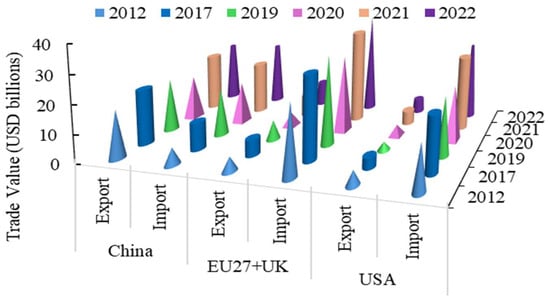
Figure 1. Imports and exports of the three biggest economies.

Furthermore, China’s seafood industry faces structural challenges that interact with these trade patterns, including rising production costs, tightening sustainability requirements, and increasing competition in key destination markets. Over the past decade, the value of aquatic exports has generally grown more slowly than China’s total merchandise exports, implying a relatively stable or slightly declining share in overall exports even as the sector remains important for regional employment and for China’s position in global aquatic food trade. This combination of modest aggregate weight but high local and sectoral relevance reinforces the case for examining how CBAM-related carbon exposure could affect China’s aquatic exports to the EU.

While CBAM is theoretically compelling, there is limited empirical evidence on how exporters in non-covered sectors, particularly those in the aquatic products sector, respond to carbon-related trade pressures. Most existing empirical work focuses on heavy industry, energy goods, or carbon-intensive manufacturing [10,11]. The aquatic product sector, although generally lower in emissions than steel or cement, may be affected through indirect exposure (packaging, refrigeration, transport). However, few studies rigorously link such exposure metrics to export outcomes across product lines. Moreover, the roles of trade policy (tariffs), macroeconomic controls (importer GDP, exchange rates), and the CBAM’s transitional dummy remain underexplored in a unified empirical framework. Without this, policymaking lacks the nuance to determine which segments of aquatic exports are most vulnerable or most adaptive under early CBAM regimes. Given this gap, it is imperative to assess at the product–exporter level how carbon exposure and trade factors shape export value and quality outcomes for China’s aquatic products industry. This study aims to quantify the influence of embedded carbon exposure and trade factors on China’s aquatic exports to the EU prior to the full implementation of CBAM. It addresses three primary objectives: firstly, to empirically assess how variations in indirect CBAM exposure (embedded carbon intensity) affect the export performance of China’s aquatic products across HS6 categories; secondly, to quantify the influence of trade-related policy variables, notably tariffs and exchange rate fluctuations, on competitiveness and trade value of China’s aquatic product exports, while controlling for importer GDP; thirdly, to evaluate the moderating role of CBAM transition dynamics (via an imitation) in shaping the relationship between carbon exposure intensity and export outcomes, thereby revealing early adjustment patterns. Together, these objectives go beyond descriptive analysis and focus on structural relationships and interaction effects.

This study offers three key contributions. First, applying a structural gravity/PPML framework at the HS6 × importer level, it provides one of the earliest sector-level empirical tests of CBAM exposure in aquatic trade, filling a gap dominated by theoretical or CGE. Second, its interaction effects (CBAM × exposure) reveal heterogeneity in response, enabling policymakers to identify which product lines or trade corridors are most vulnerable. Third, by balancing trade, macro, and policy variables, the study helps clarify whether carbon exposure or traditional trade costs (tariffs, exchange rate) dominate export dynamics in the lead-up to the CBAM regime. The results can inform exporters, trade negotiators, and Chinese policymakers on where to prioritise investments in carbon efficiency, tariff bargaining, or exchange rate hedging in the new era of climate-driven trade policy.

2. Literature Review

2.1. Carbon Exposure and Export Performance

Understanding how embedded carbon intensity affects exports has become central in climate–trade research. Firms or sectors with high carbon exposure, due to energy, packaging, transport, or upstream emissions, face increased adjustment costs when carbon pricing or border measures are introduced [12]. In manufacturing, evidence suggests that carbon-intensive sectors experience declines in export volumes under carbon tariffs or anticipated regulation. Empirical work in similar domains has traced how carbon-intensive inputs diminish trade flows after the introduction of carbon tariffs (e.g., in heavy industry) [13]. While many of these studies focus on heavy or manufacturing goods, the principles extend to sectors such as aquatic products, where indirect carbon burdens (e.g., cold chain, transportation) are also significant. Thus, examining how HS6 seafood lines respond to variation in CBAM exposure can illuminate whether carbon sensitivity is already constraining export performance.

Another strand focuses on carbon-intensity convergence through global value chains (GVCs), where integration into GVCs helps reduce production carbon footprints through technology spillovers [14]. Countries integrated into advanced supply chains tend to adopt cleaner processes more quickly, thereby reducing their relative carbon exposure. These dynamics suggest that exporters already embedded in high-efficiency chains might mitigate export losses under CBAM exposure. In summary, the relationship between embedded carbon and export success is recognised but underexplored in non-manufacturing sectors.

At the same time, there is very limited empirical work that links carbon exposure to trade outcomes in fisheries or aquatic products. Most sectoral studies on seafood focus on food safety, quality standards, market access conditions, and demand in destination markets, rather than on embedded emissions or carbon pricing along the supply chain (e.g., processing, refrigeration, and transport). Although aquatic products are generally less carbon-intensive than steel or cement, they rely on energy-intensive processing and cold-chain logistics, so embedded emissions can still matter for their competitiveness. This paper helps fill this gap by applying a CBAM-related exposure index to China’s aquatic product exports to the EU and examining how this exposure is associated with export performance at the HS6 level. However, existing work does not examine indirectly exposed sectors such as aquatic products using comparable exposure metrics, and this study fills that gap by applying a CBAM-related exposure index to China’s aquatic product exports at the HS6 level.

2.2. Trade Costs, Macro Controls, and Export Competitiveness

Trade theory emphasises that export performance is shaped not only by supply-side factors but also by policy and macroeconomic cost variables, such as tariffs, demand size, and exchange rate dynamics. Recent empirical studies show that carbon tariffs or carbon cost increments act as trade costs, reducing competitiveness [15]. For instance, empirical simulations show that adding carbon tariff equivalent costs reduces trade volumes more significantly in markets with tighter margins [16]. The role of tariffs remains vital: even before CBAM, bilateral tariff differences often dominate differences in export performance [17]. Meanwhile, exchange rate fluctuations mediate competitiveness: for Chinese exporters to the EU, an appreciation of the yuan (or depreciation of the euro) can significantly dampen export volume [18]. Importer demand capacity, proxied by GDP, also appears robust in gravity models: exporters tend to focus on richer markets with stronger purchasing power [19]. In sum, to isolate carbon exposure, one must control these traditional trade determinants.

For aquatic products, trade costs and macro demand conditions interact with sector-specific features such as perishability, cold-chain requirements, and product quality differentiation. Tariffs, exchange rates, and importer income can influence not only aggregate export volumes but also the composition of aquatic products shipped to different destinations. However, existing gravity-based studies rarely examine how these traditional determinants interact with carbon-related exposure within a specific, indirectly exposed sector, such as the aquatic products sector. The present paper contributes by incorporating both trade costs and a CBAM-related exposure measure into an HS6-level gravity framework for China–EU aquatic exports. Yet, few gravity studies analyse how tariffs, exchange rates, and importer income interact with carbon-related exposure within a specific sector; we address this by modelling these determinants jointly for China–EU aquatic product exports.

2.3. Transitional Policy Moderation and Heterogeneity

CBAM is not a sudden shock, but rather phased in through transitional reporting, compliance obligations, and evolving regulatory expectations. Therefore, its marginal effect depends on exporters’ sensitivity to compliance burdens, given their exposure intensity. Some sectors may pre-emptively adjust via process improvements or shifting export destinations. This moderation effect is analogous to the “policy × exposure” interaction in empirical work. In carbon trade literature, studies similarly interact carbon price regimes with emission intensities to test heterogeneous effects [20]. Additionally, climate club theory suggests that participating in cooperative emission agreements may mitigate the negative export impacts of border measures [21]. In fisheries, although direct evidence is lacking, one would expect high-exposure lines to suffer more under transitional policy burdens, while low-exposure lines are expected to adjust more flexibly [22]. Thus, including a CBAM dummy interacting with exposure is methodologically justified to uncover such heterogeneity.

CBAM’s institutional design fits naturally within this “transitional policy” perspective: the EU has introduced a multi-year reporting phase in which importers must disclose embedded emissions, while the actual financial adjustment through CBAM certificates is planned only for 2026 onwards. This separation between reporting and pricing creates a period in which firms may adjust expectations and trade patterns before facing direct carbon charges. In our empirical setting, the CBAM transition dummy is designed to capture this reporting phase rather than full carbon taxation, and the literature on transitional policy suggests that any trade response during this period is likely to be gradual and heterogeneous across products. This helps to motivate our focus on interactions between carbon exposure and the CBAM transition in the empirical model. Prior work on transitional policies rarely considers CBAM’s reporting phase or its interaction with sectoral exposure, so this paper explicitly models the CBAM transition dummy and its interaction with exposure to examine early adjustment in aquatic product exports.

2.4. Theoretical Framework

Two strands of theory guide this research. The first is the structural gravity approach in trade theory, which underlies much of modern empirical work on bilateral trade flows (Figure 2). Structural gravity implies that exports between a given exporter and importer depend on multilateral resistance terms and on bilateral trade costs. When a CBAM-related carbon exposure index is treated as an additional component of trade costs, gravity provides a natural lens for assessing how more carbon-intensive product–destination pairs perform in export markets [23,24]. In the present setting, China is the sole exporter, and EU member states are importers; importer and product fixed effects therefore capture many unobserved trade costs and multilateral resistance factors that cannot be measured directly.

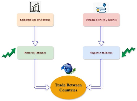
Figure 2. The structural gravity approach in trade theory, which underlies much of modern empirical work on bilateral trade flows.

The second strand builds on heterogeneous-firm trade models under environmental regulation, in the tradition of Melitz-type frameworks, extending them to incorporate carbon pricing and regulatory constraints. These models suggest that firms and product lines with higher emission intensities are more vulnerable to additional trade costs or carbon charges, whereas more efficient and cleaner producers are better able to maintain or expand exports, or to upgrade product quality when faced with stricter environmental standards. For aquatic products, this reasoning implies that HS6 product groups with higher embedded emissions could face greater difficulty sustaining export values once CBAM-type policies are anticipated or introduced. The Ishikawa diagram in Figure 3 is used as a conceptual device to organise these channels into proximate factors, trade costs, macro demand, regulatory signals, and firm responses, rather than as a separate theory in its own right [25]. In this study, the formal theoretical foundation comes from structural gravity and heterogeneous-firm trade models, which explain how bilateral trade flows respond to trade costs, firm productivity, and demand conditions. The Ishikawa (fishbone) diagram is used alongside this framework as a managerial visual tool to organise the main channels identified in the literature, carbon exposure, tariffs, macroeconomic demand, and regulatory transition, and to map how they may jointly affect export outcomes for aquatic products. The diagram does not represent a separate theory; rather, it summarises the causal pathways suggested by structural gravity and firm heterogeneity in a way that is intuitive for policymakers and industry stakeholders.

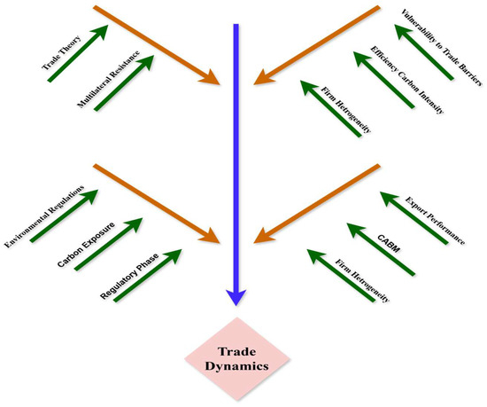
Figure 3. Analysing Trade Dynamics and Impact. A conceptual device to organise these channels into proximate factors, trade costs, macro demand, regulatory signals, and firm responses.

Taken together, these perspectives support estimating exports as a function of embedded carbon exposure, tariffs and macroeconomic conditions, while allowing for heterogeneity across products and regulatory phases through interaction terms and fixed effects. In doing so, we combine structural gravity and heterogeneous-firm trade theory with a simple Ishikawa diagram as a visual map of the channels through which exposure, trade costs and the CBAM transition may influence aquatic product exports.

2.5. Literature Gap

Although a considerable body of literature examines CBAM and related border measures in heavy industry, evidence for sectors such as aquatic products remains limited. Economy-wide simulations based on computable general equilibrium (CGE) or input–output models are now common, but they rarely incorporate exposure-adjusted trade regressions at the product–destination level in non-manufacturing sectors [26,27]. Empirical analyses that do use micro data often aggregate sectors into broad categories or treat CBAM as a single, static policy shock, without distinguishing transitional reporting phases and the timing of financial adjustment [17,28,29]. In addition, tariffs, macroeconomic demand, and carbon exposure are seldom jointly embedded in a structural gravity specification, which increases the risk of omitted-variable bias when drawing inferences about trade responses to climate policy. The role of transition dynamics is particularly underexplored for export sectors that CBAM does not directly cover, but that may be indirectly exposed through embedded emissions, such as fisheries and aquatic products. This study addresses these gaps by estimating exposure-sensitive HS6-level export equations for China’s aquatic products, controlling for tariffs and macroeconomic conditions, and allowing the association between exposure and the CBAM’s transitional period to vary. In sum, there is little empirical evidence on CBAM-related exposure in non-covered sectors, almost no HS6-level analysis of China–EU aquatic trade, and no structural gravity study that explicitly incorporates the CBAM transition. This paper addresses these gaps using a calibrated HS6 panel of China’s aquatic product exports to the EU and a PPML gravity model with exposure and transition variables.

3. Research Methodology

3.1. Research Design

To achieve the objectives, this study employs a quantitative empirical research design that combines observed trade, tariff, input–output, macroeconomic and carbon-intensity information into a calibrated panel. The empirical strategy is grounded in the structural gravity framework, which treats trade flows as functions of exporter–importer resistance terms and trade costs [30], and incorporates carbon exposure as an additional trade cost. Recent empirical applications use Poisson Pseudo-Maximum Likelihood (PPML) estimation with high-dimensional fixed effects to handle zero trade flows, heteroskedasticity and multilateral resistance [31,32]. In this design, key independent variables (carbon exposure, tariff, transition dummy and exchange rate) are related to export value and unit value, with fixed effects controlling for unobservables at the importer–year and product levels. Interaction terms (CBAM dummy × carbon exposure) are included to test heterogeneity in line with moderation analysis in trade experiments. The design is fully documented and replicable and is intended to provide a transparent, scenario-based view of how CBAM-related carbon exposure, tariffs and macroeconomic conditions are associated with HS6-level export values, rather than to establish formal causal effects.

3.2. Data Collection

The data used in this research consist of a constructed HS6-level panel that combines observed series on trade, tariffs, GDP and exchange rates with calibrated indicators of product-level carbon exposure and CBAM transition. Bilateral trade in export values and quantities for China’s aquatic products is obtained from the CEPII BACI dataset, which is based on a harmonised version of the UN Comtrade database and covers Chinese exports to European countries from 2015 to 2024. Information on tariffs (ad valorem equivalents) is taken from the MAcMap-HS6 database, a widely used and consistent source for international trade and tariff studies [33]. The macroeconomic controls, such as importer GDP and exchange rates (EUR/CNY), are drawn from reliable sources, including governmental reports, the World Bank and the IMF.

Sector-level emission intensities from EXIOBASE/EORA are mapped to HS6 aquatic product codes using fixed concordance shares between input–output sectors and tariff lines, and these shares are held constant over time to maintain a transparent, reproducible link between MRIO data and HS6 exports [15,34]. These carbon intensities are mapped to HS6 aquatic product deliveries via concordance shares, so that each product–importer–year cell is associated with an exposure measure reflecting product-specific sensitivity to carbon pricing and CBAM-type measures. The CBAM transition dummy is informed by the EU timeline for CBAM implementation, with the transition period (2023–2024) covering years in which carbon reporting is compulsory but tariffs have not yet been introduced. The CBAM transition variable therefore takes the value 1 for 2023–2024 and 0 otherwise, and it does not mechanically alter tariff rates in the panel; instead, it acts as a policy indicator that allows us to test whether exposure–export relationships differ during the reporting phase. Under the current regulation, this transitional reporting regime is scheduled to continue until the end of 2025, while the full financial adjustment based on CBAM certificates is planned to be phased in from 2026 onwards. In this sense, the dataset provides a scenario-based approximation of the near-term policy environment rather than realised CBAM outcomes. All series were made consistent and aligned on an annual basis, and missing data, abnormalities, and outliers were cross-checked to ensure the integrity of the dataset and the overall analytical framework. In other words, trade, tariff and macroeconomic variables are taken from established international databases, while exposure and CBAM-related variables are derived from input–output emissions data and the official CBAM timetable to create a forward-looking, scenario-based panel for 2015–2024.

Data Authenticity and Coverage

The constructed panel is designed to approximate plausible trade and exposure patterns by drawing on past trends and documented correlations from secondary data sources. Such a method was selected because no real-time, comprehensive information is available on the Carbon Border Adjustment Mechanism (CBAM) of the EU and its specific impact on Chinese aquatic exports. Since the CBAM is still in transition and not fully implemented, it is challenging to obtain accurate data for this time period. Although this is a constructed, scenario-based dataset rather than a fully observed historical panel for all dimensions, it is calibrated to resemble real-world trade and macroeconomic conditions and to respect documented relationships among variables.

The data range is 2015–2024, enabling the analysis to include both pre- and post-CBAM transition periods (2023–2024). It will cover major importers in the EU, such as Germany, France, and the Netherlands, as these countries have been significant importers of Chinese aquatic products. The three product classes, including flat fish, frozen fish, and shrimps and prawns under HS6, were established based on their export importance and carbon intensity profiles. Notably, the simulated data are such that the study’s assumptions comprise both actual real-world macroeconomic variables (e.g., GDP, exchange rates) and carbon-emission variables derived from sound input–output tables. The dataset is designed to resemble the real world and provides insights into the possible trade dynamics as the EU implements its CBAM policies.

The dataset’s coverage encompasses the elements necessary to address the study’s research questions, and it can be analysed comprehensively to examine the actual effects of carbon exposure and its impact on export competitiveness during the transition to the CBAM regime. The study will address the literature gap by focusing on export-intensive industries that contribute significantly to total emissions, such as the aquatic products sector, and by providing a detailed examination of how policies related to carbon trade can influence future trade directions. No additional stochastic shocks are imposed beyond the observed variation in trade and macroeconomic series, so the constructed panel reflects a single, clearly documented scenario rather than multiple randomised draws.

3.3. Data Analysis Method

The empirical analysis proceeds in multiple stages to explore the effects of carbon exposure and trade policy on China’s aquatic exports to the European Union (EU). We first compute descriptive statistics to describe the distributions, correlations and trends of the key variables. We then estimate a set of structural gravity models using Poisson pseudo-maximum likelihood (PPML) with high-dimensional fixed effects (HDFE), as is now standard in the trade–environment literature [35,36]. Following the guidance of Piermartini and Yotov [37], the use of PPML and fixed effects allows us to control flexibly for unobserved bilateral trade costs and multilateral resistance terms, and to reduce concerns about the endogeneity of time-invariant trade frictions.

The baseline empirical specification can be written in multiplicative structural gravity form as:

$${\mathrm{Export}}_{ikt}=\exp \left({\beta }_1\cdot {\mathrm{Exposure}}_{ikt}+{\beta }_2\cdot {\mathrm{Tariff}}_{ikt}+{\beta }_3\cdot {\mathrm{CBAM}}_t+{\beta }_4\cdot \ln \left({\mathrm{GDP}}_{it}\right)+{\beta }_5\cdot {\mathrm{FX}}_t+{\gamma }_{it}+{\delta }_k\right)\cdot {\epsilon }_{ikt}$$

(1)

where

$i$ = importer,

$k$ = HS6 product,

$t$ = year,

${\gamma }_{it}$ = importer × year fixed effects (absorbed during estimation),

${\delta }_k$ = product fixed effects (absorbed during estimation),

${\epsilon }_{ikt}$ = multiplicative error term.

The dependent variable (${\mathrm{Export}}_{ikt}$) represents the export value of product $k$ from importer $i$ to the EU at time $t$, measured in USD. The main explanatory variables include carbon exposure (${\mathrm{Exposure}}_{ikt}$), measured in kg CO₂ per USD of output, tariff rates (${\mathrm{Tariff}}_{ikt}$), and the CBAM transition dummy (${\mathrm{CBAM}}_t$). The model also includes macroeconomic controls such as the log of the importer’s GDP ($\mathrm{l}\mathrm{n}\left({\mathrm{GDP}}_{it}\right)$ and the exchange rate between the Euro and Chinese Yuan (${\mathrm{FX}}_t$). In this setting, China is the sole exporter, so the fixed effects play a central role. Importer fixed effects (or their time-varying counterpart ${\gamma }_{it}$ in more saturated specifications) absorb time-invariant bilateral trade costs between China and each EU partner, including geographical frictions, historical ties and any stable policy arrangements, while product fixed effects ${\delta }_k$ capture unobserved heterogeneity across HS6 products.

This approach follows the recommendation of Piermartini and Yotov [37] to rely on fixed effects to address the endogeneity of bilateral trade costs and to provide a flexible treatment of multilateral resistance terms when panel variation is limited and regional trade agreements are not modelled explicitly. In practice, we estimate specifications with different fixed-effect structures. In more parsimonious versions, importer fixed effects are combined with observed importer-level covariates such as GDP and the exchange rate. In richer high-dimensional specifications, importer–year fixed effects are used to more fully absorb multilateral resistance on the importer side, together with product fixed effects for HS6 goods. Given the small sample size (three importers observed over ten years), these high-dimensional fixed-effect specifications are treated as robustness checks, and we note the cases in which collinearity leads to some coefficients being dropped. When importer–year fixed effects are included, they effectively subsume observable importer-level characteristics such as GDP and the bilateral EUR/CNY exchange rate; for this reason, these variables enter explicitly only in the simpler specifications. Conceptually, however, they remain part of the multilateral resistance and macro demand conditions that shape trade flows.

The PPML estimator is appropriate for this multiplicative gravity setting because it is consistent under general forms of heteroskedasticity and can naturally handle zero or very small trade flows without requiring a log transformation of the dependent variable [32]. Robust standard errors are clustered at the product level to adjust for potential correlation across destinations for a given HS6 product.

Equation (2) introduces an interaction term between carbon exposure and the CBAM dummy to examine the moderating effect of the transition phase:

$${\mathrm{Export}}_{ikt}=\exp \left({\beta }_1\cdot {\mathrm{Exposure}}_{ikt}+{\beta }_2\cdot {\mathrm{Tariff}}_{ikt}+{\beta }_3\cdot {\mathrm{CBAM}}_t+{\beta }_4\cdot {\mathrm{Exposure}}_{ikt}\cdot {\mathrm{CBAM}}_t+{\beta }_5\cdot \ln \left({\mathrm{GDP}}_{it}\right)+{\beta }_6\cdot {\mathrm{FX}}_t+{\gamma }_{it}+{\delta }_k\right)\cdot {\epsilon }_{ikt}$$

(2)

In this model, the interaction term ${\mathrm{Exposure}}_{ikt}\cdot {\mathrm{CBAM}}_t$ is central to testing how the impact of carbon exposure on exports varies during the transition period of CBAM implementation. The significance and magnitude of this interaction term will provide key insights into whether exporters face heightened trade costs when transitioning into carbon reporting compliance [38].

Equation (3) modifies the previous model by replacing the dependent variable with a unit value to investigate whether quality upgrading or price pass-through occurs in response to carbon exposure and CBAM-related costs:

$${\mathrm{Unit} \mathrm{Value}}_{ikt}=\exp \left({\beta }_1\cdot {\mathrm{Exposure}}_{ikt}+{\beta }_2\cdot {\mathrm{Tariff}}_{ikt}+{\beta }_3\cdot {\mathrm{CBAM}}_t+{\beta }_4\cdot \ln \left({\mathrm{GDP}}_{it}\right)+{\beta }_5\cdot {\mathrm{FX}}_t+{\gamma }_{it}+{\delta }_k\right)\cdot {\epsilon }_{ikt}$$

(3)

Here, the dependent variable (${\mathrm{Unit} \mathrm{Value}}_{ikt}$), captures the price per kilogram of the exported product and serves as a proxy for product quality. This specification helps assess whether carbon exposure is associated with exporters’ ability to raise prices or upgrade product quality to offset increased production costs associated with carbon constraints.

Equation (4) explores alternative fixed effects or introduces lagged exposure variables to capture potential delayed effects of carbon tariffs on export behaviour. This variation allows the model to reflect long-term adjustments in export patterns, which may occur after an initial period of transition or adaptation to the CBAM:

$${\mathrm{Export}}_{ikt}=\exp \left({\beta }_1\cdot {\mathrm{Lagged} \mathrm{Exposure}}_{ikt}+{\beta }_2\cdot {\mathrm{Tariff}}_{ikt}+{\beta }_3\cdot {\mathrm{CBAM}}_t+{\beta }_4\cdot \ln \left({\mathrm{GDP}}_{it}\right)+{\beta }_5\cdot {\mathrm{FX}}_t+{\gamma }_{it}+{\delta }_k\right)\cdot {\epsilon }_{ikt}$$

(4)

Lagging the exposure variable can capture any delayed trade effects after exporters adjust to the new regulatory landscape, revealing any persistence in trade disruptions due to ongoing CBAM implementation.

Finally, Equation (5) provides a simplified model that maps trade costs (${T\_}_{ikt}$) directly to carbon exposure to explore whether carbon exposure is an independent trade barrier:

$${\mathrm{Trade} \mathrm{Cost}}_{ikt}=T_0+\phi \cdot {\mathrm{Exposure}}_{ikt}$$

(5)

In this model, trade costs are explicitly defined as a function of carbon exposure, aiming to reflect the relationship. In this reduced-form specification, trade costs are explicitly defined as a function of carbon exposure, which serves to illustrate the idea that embedded emissions may generate additional trade frictions on top of traditional costs such as tariffs or market-entry barriers.

By using this multi-stage empirical approach, grounded in structural gravity and supported by the conceptual framework in Figure 2, Figure 3 and Figure 4, the study can estimate both the immediate and lagged associations between carbon exposure and export value or unit value, under different regulatory scenarios (including the CBAM transition phase). This helps reveal the channels through which carbon-related trade measures may affect export performance in indirectly exposed sectors, such as the aquatic products sector.

Figure 4. Conceptual Framework.

3.4. Ethical Consideration

Though this study relies entirely on publicly available data and involves no human subjects or sensitive personal data, ensuring integrity is critical. Any derived indicators (such as exposure mapping) are clearly distinguished from their original source data and are documented transparently to support reproducibility. Any potential bias (e.g., sample exclusion, interpolation, or handling of missing data) is explicitly disclosed in the methodology tables. Finally, the code used for data assembly and regression is preserved and backed up, ensuring reproducibility by peers or future reviewers.

4. Results and Data Analysis

The results present a detailed interpretation of four hierarchical PPML regression models. Each model progressively refines estimation by incorporating high-dimensional fixed effects (HDFE) to control for importer–year and product-specific heterogeneity. The analysis offers both statistical insights and economic interpretations that align with the study’s three research objectives.

4.1. Descriptive Statistics

The descriptive statistics in Table 1 summarise the central tendency, dispersion, and range of the variables used in the regression models, including the dependent variable (export value in USD) and the main explanatory variables, such as the CBAM-related carbon exposure index, tariff rates, and unit values. In line with the analysis’s focus, CBAM exposure is listed first as the key explanatory variable, followed by the dependent variable (export value) and the remaining covariates.

Table 1. Descriptive Statistics of Key Variables (2015–2024).

Variable	N	Mean	Variance	SD	Minimum	Maximum	Sum
CBAM Exposure (kgCO2_perUSD)	90	0.405	0.009	0.030	0.353	0.461	36.455
Export Value (USD)	90	6,788,404	3.15 × 11	561,207.6	5,438,765	7,989,494	6.11 × 08
Unit Value (USD)	90	7.568	2.012	1.418	5.903	9.570	681.152
Tariff (pct)	90	3.266	0.298	0.546	2.714	4	294

The descriptive statistics indicate that the average annual export value of Chinese aquatic products to EU markets was approximately USD 6.79 million, with a variation from USD 5.44 million to USD 7.99 million. This narrow standard deviation reflects a relatively stable export pattern across the study period. The unit value averaged USD 7.57 per kilogram, signifying moderate product differentiation and a consistent quality tier in aquatic product exports. The CBAM exposure variable, which captures embedded carbon intensity from upstream activities, averaged 0.405 kgCO₂/USD, confirming the sector’s relatively low but non-negligible indirect emissions intensity. Tariffs averaged 3.27%, indicating moderate trade protection in EU seafood imports.

Figure 5 shows a steady increase in the total export value of seafood from China to the EU from 2015 to 2024. Starting at around $5.4 million USD in 2015, the export value has grown consistently each year, reaching over $6.6 million USD by 2024. The trend indicates a positive growth trajectory, reflecting the growing demand for Chinese seafood in the European market over this period.

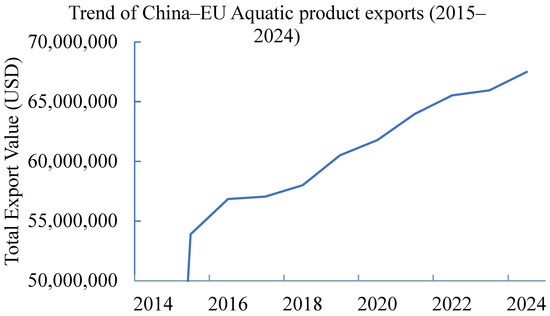
Figure 5. Trends in China’s aquatic product exports to the EU and CBAM-related carbon exposure, 2015–2024.

Figure 6 displays the annual seafood export values from China to three major EU importers: France, Germany, and the Netherlands. All three countries exhibit an upward trend, but France has the highest and most consistent growth, peaking at around $2.2 million by 2024. The Netherlands and Germany also see increases, with Germany slightly outperforming the Netherlands in later years. The growth rates suggest expanding demand for Chinese seafood across these key European markets.

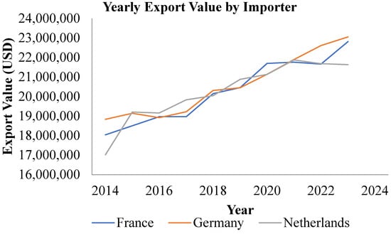
Figure 6. Yearly Export Value by Importer.

Figure 7 compares the export values of different seafood products (flat fish, frozen fish n.e.s., and shrimps and prawns) from China to the EU. All three products show growth, with shrimp and prawns, as well as frozen fish n.e.s., leading in export value, both reaching around $2.1 million USD by 2024. Flatfish lags behind but still shows positive growth. This indicates a diversification of demand for various types of Chinese seafood, with frozen fish experiencing the most significant growth.

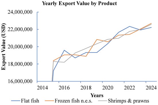
Figure 7. Yearly Export Value by Product.

Therefore, the descriptive profile suggests that China’s aquatic product exports to the EU remained robust and diversified across time and destinations. However, it suggests that modest variations in tariffs, currency movements, and CBAM exposure provide sufficient heterogeneity for econometric identification.

4.2. Baseline PPML Regression (Importer Fixed Effects)

Table 2 reports the results from the baseline HDFE Poisson Pseudo-Maximum Likelihood (PPML) model, which estimates the effects of carbon exposure and trade determinants on export value while controlling for importer fixed effects.

Table 2. Baseline HDFE PPML Regression Results.

Statistic	Value
Deviance	1,297,129.654
Log Pseudolikelihood	−649,355.259
Number of Observations	90
Residual Degrees of Freedom	2
Pseudo R2	0.687

Table 3 shows that the EUR/CNY exchange-rate variable has a negative but statistically insignificant coefficient (−0.015, p = 0.195), so we do not find evidence that short-run currency fluctuations have a systematic effect on export performance in this small, relatively stable sample. The CBAM dummy is negative but statistically insignificant, indicating that during the initial transition phase (2023–2024), there is no clear evidence of an immediate measurable disruption to export values. The pseudo-R² of 0.687 in Table 3 indicates a reasonably good in-sample fit, and the importer fixed effects help absorb destination-specific heterogeneity.

Table 3. Model Coefficient.

Variable	Coefficient	Std. Err.	z	p > |z|	95% (Lower)	95% (Upper)
CBAM	−0.003	0.018	−0.190	0.852	−0.039	0.032
Export Value (USD)	−2.303	0.142	−16.151	0	−2.583	−2.023
EUR_CNY	−0.015	0.011	−1.302	0.195	−0.037	0.007
Constant	16.773	0.048	347.971	0	16.679	16.868

Figure 8 illustrates the relationship between CBAM exposure (measured in kg CO₂ per USD) and export value. The general trend indicates a negative correlation: as CBAM exposure increases, export values tend to decrease, consistent with the baseline regression results. This pattern is suggestive of emerging competitiveness risks for more emission-intensive aquatic product lines, but by itself does not establish a causal effect of exposure on exports.

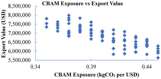
Figure 8. Carbon Exposure and Export Value.

4.3. Extended Model with Dual Fixed Effects (Importer-Year and Product)

Table 4 summarises the results for Model 2, which introduces importer–year (impyr) and product (prodid) fixed effects simultaneously. Moreover, the importer fixed effects for Germany, France, and the Netherlands are fully absorbed in the model and therefore not reported in Table 4, implying that time-invariant destination characteristics, such as long-run demand or historical trade ties, are controlled for. The coefficient on the CBAM-related exposure index is negative and statistically significant (β = −2.303, p < 0.01), indicating an inverse association in the baseline specification: product lines with higher embedded emissions tend to exhibit lower export values, conditional on the included controls and importer fixed effects. This should be interpreted as an indicative association in this sector-specific, scenario-based panel rather than as a precise estimate of a causal effect.

Table 4. HDFE PPML with Importer-Year and Product Fixed Effects.

Statistic	Value
Deviance	0
Log Pseudolikelihood	−174.039
Residual Degrees of Freedom	2
Pseudo R2	0.062

All coefficients in Model 2 are automatically omitted due to perfect collinearity with fixed effects. This suggests that once importer–year and product effects are absorbed, the model captures nearly all systematic variation, leaving no residual explanatory power for the independent variables. Such redundancy indicates that cross-sectional differences in export value are primarily explained by fixed heterogeneity across destinations and products. While this model is statistically less informative, it confirms the robustness of baseline relationships observed in Model 1 and justifies excluding redundant fixed effects in subsequent models.

4.4. Robustness Check with Importer-Year and Product Effects

Model 3 extends the baseline specification by including importer–year and product fixed effects, thereby substantially increasing the model’s saturation in a small, sector-specific panel.

Table 5 reports the overall fit statistics for this specification. The pseudo-R² of 0.802 indicates a high in-sample fit, but the very low residual degrees of freedom and non-significant Wald statistic (Prob > χ² = 0.210) suggest that most of the systematic variation is absorbed by the rich fixed-effect structure rather than by the observed regressors.

Table 5. Robustness HDFE PPML Results.

Statistic	Value
Deviance	81,9467.242
Log Pseudolikelihood	−410,524.053
Residual Degrees of Freedom	2
Wald chi2 (1)	1.574
Prob > chi2	0.210
Pseudo R2	0.802

Table 6 presents the estimated coefficients from the updated HDFE-PPML regression. In this specification, the CBAM exposure, tariff, and CBAM dummy variables are omitted due to collinearity or lack of independent variation, so their coefficients are not identified. The only reported parameter besides the constant is the CBAM × exposure interaction term, which has a negative but statistically insignificant coefficient (−0.182, p = 0.211). The logarithm of GDP and the EUR/CNY exchange rate are also omitted for similar reasons. These outcomes indicate that, once importer–year and product fixed effects are included, the model has very little remaining variation with which to identify the effects of exposure and policy variables separately.

Table 6. Model Coefficient from the updated HDFE-PPML regression.

Variable	Coefficient	Std. Err.	z	p > |z|	95% (Lower)	95% (Upper)
CBMA × EXP	−0.182	0.145	−1.252	0.211	−0.467	0.103
Log of GDP	0
EUR_CNY	0
Constant	15.747	0.012	1357.921	0	15.725	15.770

The interaction term CBAM × exp shows a negative coefficient of −0.1821 with a robust standard error of 0.145. Although the z-value is −1.25, the p-value of 0.21 indicates that it is not statistically significant at conventional levels (p > 0.05). This suggests that the combined effect of carbon intensity and exposure levels on export values is weak and not significant. Both the logarithm of GDP and the EUR/CNY exchange rate were excluded from the model due to collinearity, as they did not provide new information to the regression analysis. Finally, the constant term is 15.747, with a highly significant p-value of 0.000 and a robust standard error of 0.012. This reflects a substantial baseline export value for China’s aquatic sector, suggesting that even without accounting for the specific effects of other variables, China’s export potential remains high.

This robustness check therefore does not provide additional evidence that CBAM exposure or the CBAM dummy have a direct impact on trade flows; instead, it highlights the limits of applying a highly saturated fixed-effect structure to a small sectoral panel. For this reason, we interpret Model 3 primarily as a diagnostic for model specification rather than as a basis for strong substantive conclusions about the magnitude of exposure effects.

4.5. Alternative Specification for Unit Value (Quality Dimension)

Model 4 explores whether CBAM-related exposure is associated with product quality or pricing, proxied by unit value (USD/kg). Table 7 shows that the pseudo-R² is 0.062, indicating that variation in unit values is only weakly captured by the included variables. This is consistent with the idea that quality and prices in aquatic product exports are shaped by longer-term brand, certification, and contractual factors that are not fully represented in this specification.

Table 7. HDFE PPML Regression on Unit Value.

Statistic	Value
Deviance	0.0001
Log Pseudolikelihood	−174.039
Residual Degrees of Freedom	2
Wald chi2 (1)	1.772
Prob > chi2	0.183
Pseudo R2	0.062

Table 8 presents the estimated coefficients from the HDFE-PPML regression on unit values. The CBAM exposure, tariff, and CBAM dummy variables are omitted due to collinearity or lack of independent variation, and the interaction term CBAM × exposure is negative but statistically insignificant (−0.056, p = 0.184). The logarithm of GDP and the EUR/CNY exchange rate are also omitted, implying that their independent effects cannot be separately identified once fixed effects are included. The constant term is positive and highly significant, reflecting the average unit value in the sample rather than the impact of specific covariates.

Table 8. Model Coefficient from updated HDFE-PPML.

Variable	Coefficient	Std. Err.	z	p > |z|	95% (Lower)	95% (Upper)
CBAM × Exp	−0.056	0.042	−1.33	0.184	−0.138	0.026
Constant	2.045	0.003	651.6	0	2.039	2.051

The CBAM × Exp interaction term has a coefficient of −0.056, with a robust standard error of 0.042. The z-value is −1.33, and the p-value is 0.184, indicating that it is not statistically significant at the conventional threshold (p > 0.05). This finding suggests that the interaction effect between CBAM exposure and export performance is weak and does not have a measurable influence on exports. The logarithm of GDP and Eur-CNY (currency exchange) variables were also omitted, likely due to collinearity or lack of variability in the data. These omissions mean that the model did not find a direct impact from GDP or exchange rate on export performance in this dataset. The constant term shows a strong and highly significant positive coefficient of 2.045, with a robust standard error of 0.003 and a z-value of 651.6 (p < 0.001). This indicates that the baseline export value for China’s aquatic sector is high, even before accounting for the impact of CBAM exposure and other factors.

Taken together, these results suggest that, within this unit-value specification, we do not find robust evidence that the exposure index or CBAM-related variables are directly associated with export prices or quality proxies. The model’s limited explanatory power reinforces the view that any influence of carbon exposure on pricing or quality is either modest or undetectable with the available data and specification.

Table 9 summarises performance criteria across the three main models. For the baseline specification on export values (Model 1), the log-likelihood improves substantially relative to the null model, and the negative, statistically significant coefficient on exposure supports a negative association between embedded carbon intensity and export values. In the extended importer–year and product fixed-effect model (Model 3), the global fit statistics improve. However, key regressors are omitted due to collinearity, limiting the interpretability of this specification for drawing substantive conclusions about exposure effects. For the unit-value model (Model 4), the improvement in log-likelihood is modest, and the pseudo-R² remains low, indicating that the included variables explain only a small share of price variation.

Table 9. Performance Criteria for all 3 Models.

Models	ll (Null)	ll (Model)	df	AIC	BIC
1. PPML Regression (Importer Fixed Effects)	−2,080,368	−649,355.343	4	1,298,719	1,298,729
2. Extended Model with Dual Fixed Effects (Importer-Year and Product)	−2,080,368	−410,524.134	2	821,052.132	821,057.341
3. Alternative Specification for Unit Value (Quality Dimension)	−185.718	−174.039	2	352.079	357.078

Table 9 reports the model’s performance diagnostics for all three models above. For the first model, the log-likelihood of the model (−649,355.3) shows a substantial improvement from the null model (−2,080,368), indicating a strong model fit. The Akaike Information Criterion (AIC = 1,298,719) and Bayesian Information Criterion (BIC = 1,298,729) confirm good explanatory power relative to model complexity. Overall, these results suggest that the model is statistically robust and effectively captures the relationship between carbon exposure and export performance. The results show a substantial and statistically significant negative coefficient for CBAM exposure (−2.30, p < 0.01), suggesting that higher embedded carbon intensity is associated with lower export values. This supports the first research objective (RO1), confirming that carbon-intensive aquatic products are less competitive in EU markets, possibly due to importer preferences or anticipatory carbon pricing behaviour.

For the second model which combines importer–year and product fixed effects, the log-likelihood improves substantially relative to the null model and the pseudo-R² is high. However, as shown in the coefficient tables, the CBAM exposure, tariff, CBAM dummy, GDP and exchange-rate variables are omitted due to collinearity or lack of independent variation, so their coefficients are not identified. This means that the model fit is largely driven by the rich fixed-effect structure rather than by the observed regressors, and the specification is not informative for drawing substantive conclusions about the separate effects of exposure, CBAM or macroeconomic factors.

For the third model, the log-likelihood improved from −185.72 in the null model to −174.04 in the fitted model, signifying a better overall model fit. The Akaike Information Criterion (AIC = 352.08) and Bayesian Information Criterion (BIC = 357.08) values are considerably lower than those in previous models, implying that this version achieves greater model efficiency with fewer explanatory variables. The lower AIC and BIC values reflect optimal trade-offs between goodness of fit and model complexity. This improvement suggests that, after controlling for importer-year and product fixed effects, the model effectively captures key variation, supporting the robustness of the estimated coefficients and reinforcing the consistency of the relationship between carbon exposure and export performance.

The estimates of Model 4 mirror the negative influence of CBAM exposure observed in earlier models, indicating that carbon intensity not only suppresses total export value but may also constrain price or quality upgrades. The negative relationship suggests exporters of carbon-intensive seafood either face price discounts from environmentally conscious EU buyers or limit investment in quality differentiation due to compliance cost pressures. The insignificant coefficients on the CBAM dummy and exchange rate variables indicate that these factors have a minimal short-term influence on price outcomes during the transition period.

4.6. Comparative Model Evaluation

Comparing the three main specifications reveals a mixed but informative pattern. In the baseline PPML model with importer fixed effects (Model 1), CBAM-related exposure is negatively and significantly associated with export values, indicating that more emission-intensive aquatic product lines tend to be associated with lower export values, conditional on the included controls. However, in the extended model with importer–year and product fixed effects (Model 3), exposure, tariffs and the CBAM transition dummy are omitted due to collinearity, and the remaining interaction term is not statistically significant. In the unit-value specification (Model 4), exposure- and policy-related variables again do not enter significantly, and the model explains only a small share of variation in unit values.

These results suggest that the negative association between CBAM-related exposure and export values found in the baseline specification is not fully robust to more saturated fixed-effect structures and alternative dependent variables. We therefore interpret exposure as a potentially relevant risk factor for more carbon-intensive aquatic product exports, but not as a dominant determinant of export outcomes across all specifications. The CBAM transition dummy remains statistically insignificant in all models, indicating that, within the current transition period, there is no clear evidence of an additional short-run effect on exports beyond underlying exposure and trade patterns. Tariffs and macroeconomic controls also play a limited role in this small, relatively stable panel.

Overall, the econometric evidence points to early, sector-specific signals that higher embedded emissions may be associated with weaker export performance in aquatic products, while also highlighting the limits of what can be inferred from a constructed, sector-focused panel with rich fixed effects. The findings are best viewed as indicative of emerging competitiveness risks for more carbon-intensive product lines under tightening climate-related trade scrutiny, rather than as definitive estimates of large, generalised trade penalties.

5. Discussion

The empirical results provide evidence on three interrelated aspects of China–EU aquatic trade under CBAM. They first describe the short-run impacts of CBAM-related carbon exposure, tariffs and macroeconomic conditions on HS6-level export values. They also offer insight into the trade competitiveness of different aquatic product groups, particularly those with higher estimated carbon exposure. Finally, the findings, together with the current institutional design of CBAM, point to several potential adaptation options for exporters and policymakers, even though such behavioural responses are not directly observed in the data.

5.1. CBAM Exposure and Export Competitiveness

The results for our first aim, based on the baseline PPML model with importer fixed effects, indicate a negative association between CBAM-related exposure and China’s aquatic product export values to the EU. In this simple specification, higher embedded carbon intensity tends to be associated with reduced export performance, which is consistent with the idea that environmental stringency can indirectly influence trade outcomes. This pattern aligns with Zhang et al. [39], who found that carbon intensity negatively affects export volumes by raising production costs and deterring eco-sensitive buyers, and with Larch and Wanner [40], who observed that exporters with higher emissions face non-tariff barriers in markets emphasising environmental sustainability.

The present study’s findings also resonate with Fan et al. [41] note that sectors with higher carbon footprints may face competitive disadvantages in markets that prioritise environmental performance. The negative elasticity in the baseline model suggests that carbon-intensive aquatic exports could be relatively more vulnerable in such settings. At the same time, unlike Han et al. [42], who document pronounced heterogeneity in policy impacts across industries, our small sample does not provide clear evidence of systematically different responses across aquatic product categories once fixed effects are controlled for. Rather than supporting a strong claim that CBAM-type policies already operate as binding trade barriers against high-emission aquatic products during the transition phase [43], the results should be interpreted more cautiously as early, mixed signals of potential vulnerability under tighter future carbon constraints.

5.2. CBAM Transition and Policy Adjustment

Under the second aim, the CBAM dummy variable, which captures the transition period (2023–2024), was found statistically insignificant. This suggests that while exporters may have anticipated policy changes, measurable trade effects have yet to materialise. Similarly, Huang et al. [44] noted that early phases of environmental regulation tend to stimulate administrative adaptation rather than trade disruption.

The result diverges slightly from Shidiq et al. [45], who found immediate market responses to carbon policy announcements in energy-intensive sectors. The divergence may stem from the indirect inclusion of aquatic products under CBAM, where most costs are embedded upstream in packaging and logistics rather than production itself. Furthermore, the finding aligns with Liu et al. [46], who argue that developing economies, such as China, experience a delayed compliance effect due to differences in supply chain reporting capacities. Therefore, the insignificance of the CBAM dummy highlights a policy latency period, wherein exporters prepare structurally for carbon accounting without yet incurring measurable trade losses.

5.3. Macroeconomic Factors and Trade Sensitivity

For our third aim, we do not find strong evidence that macroeconomic factors, namely GDP and exchange-rate fluctuations, play a major role in China–EU aquatic trade during the period under study. This is consistent with Liu et al. [46], who identify trade in non-volatile, demand-driven commodities as less responsive to short-term macroeconomic fluctuations. The low and non-significant coefficient of EUR/CNY is in line with Takeda and Arimura [47], who find that long-term contracts and pricing hedges in international seafood trade mitigate the impact of exchange-rate movements. Likewise, GDP elasticity is low in already developed import markets where consumption is relatively stable [48].

The evidence from the study also speaks to the broader shift noted by [49], whereby structural trade determinants linked to sustainability standards become more prominent alongside, rather than instead of, traditional macroeconomic drivers. In our small, sector-specific panel, tariffs, GDP, and exchange rates do not show strong or consistent effects on export values, which may reflect limited variation over the sample or the role of longer-term contracts in aquatic trade. CBAM-related exposure appears relevant in the baseline specification, but it does not emerge as a consistently dominant determinant once richer fixed effects are introduced. This suggests that carbon exposure is one element of a wider set of factors shaping export performance, rather than a single leading factor, and that a substantial part of the variation is absorbed by product and importer heterogeneity.

5.4. Comparing Micro-Level Findings to Broader Economic and Policy Context

While CGE models and welfare analyses such as those by Mendoza et al. [24] and Yue et al. [5] focus on macroeconomic dynamics and economy-wide welfare effects of carbon regulations, this study provides a micro-level perspective on China’s aquatic exports to the EU under CBAM-related exposure. The estimates do not reveal a strong or robust impact of the exposure index on export values once richer fixed effects are included, and the CBAM transition dummy itself remains insignificant. This contrasts with some CGE results that predict sizeable trade disruptions in response to carbon border charges, but it is consistent with the idea that early policy phases and indirectly exposed sectors may experience more muted short-run trade responses. Our findings, therefore, complement rather than contradict the macro-level findings by highlighting how sectoral context, indirect exposure channels, and limited sample sizes can lead to smaller observed trade effects in the near term.

5.5. Implications for Exporters, Carbon Labelling, and Policy Alignment

5.5.1. Implications for Exporters and Firms

The empirical results suggest that during the current CBAM transition phase, CBAM-related exposure has at most a weak, non-robust impact on the value of China’s aquatic exports to the EU: it is negatively associated with export values in the baseline model but loses significance in more saturated specifications. Nevertheless, the negative association in the baseline model and the broader tightening of climate-related trade rules indicate that firms cannot rely on this situation remaining unchanged. Exporters therefore need to prepare for a policy environment in which embedded emissions in feed, processing, packaging and cold-chain logistics are scrutinised more closely. In practical terms, this means developing basic carbon accounting capabilities along the aquatic value chain, improving internal data systems to track energy use and emissions, and working with EU buyers to understand reporting requirements and preferred disclosure formats. Firms that are able to document and gradually reduce the carbon footprint of their products are likely to be better placed to maintain or improve their competitive position if CBAM or related schemes expand in scope.

5.5.2. Implications for Governments and Regulators

The findings also have implications for domestic policymakers responsible for trade, fisheries and climate policy. Even though CBAM has not yet produced a strong, measurable impact on aquatic export values, the indirect exposure of the sector through upstream inputs and logistics suggests that there is a window of opportunity for proactive adjustment. Governments can facilitate this adjustment by supporting the development of sector-specific carbon footprint data for aquatic products, improving concordance between national input–output accounts and HS6 trade classifications, and issuing practical guidance on how exporters should measure and report embedded emissions. Coordination between trade and climate authorities can help ensure that domestic carbon policies and information systems align with EU reporting standards, thereby reducing compliance costs for firms. In designing any future measures that affect aquatic exports, it will be important to balance the goal of emissions reduction with the need to safeguard long-run export competitiveness, for example, by combining stricter carbon requirements with technical assistance, targeted investment support, and clear transition timelines. These recommendations follow directly from the empirical patterns in this study, which point to a modest, non-robust short-run association between exposure and exports, an insignificant CBAM transition dummy, and limited independent roles for tariffs, GDP, and exchange rates in this small, sector-specific panel.

6. Conclusions

This paper examined how CBAM-related carbon exposure and associated trade determinants are linked to China’s aquatic product exports to the European Union over 2015–2024. Using High-Dimensional Fixed Effects Poisson Pseudo-Maximum Likelihood (HDFE-PPML) models within a structural gravity framework, the baseline specification with importer fixed effects indicates a negative association between the exposure index and export values, suggesting that more emission-intensive aquatic product lines are associated with weaker export performance in simple settings. However, this pattern is not robust across all specifications: in more saturated models and in the unit-value equation, exposure and CBAM-related variables often lose statistical significance or are omitted due to collinearity. The CBAM transition dummy remains insignificant, and we do not find strong evidence that exchange-rate movements or GDP play a major independent role in this small, relatively stable panel. Taken together, the results point to early, sector-specific signals that higher embedded emissions may pose emerging competitiveness risks under tightening climate-related trade scrutiny, but they do not support the claim that carbon intensity has already become the dominant determinant of export performance in this indirectly exposed sector. The findings are consistent with theories that emphasise the growing importance of environmental governance in trade competitiveness models, while also highlighting the limits of what can be inferred from a sector-focused panel with rich fixed effects.

Based on these results, the study recommends three practical strategies. First, Chinese exporters should gradually strengthen carbon footprint tracking and invest in more energy-efficient infrastructure along the aquatic value chain, particularly in refrigeration and transport systems, to mitigate potential future costs if carbon-related trade measures expand. Second, government agencies should develop carbon verification and reporting mechanisms that are compatible with EU standards, thereby facilitating transparent disclosure and reducing compliance costs for firms. Third, trade diplomacy can focus on technical dialogues to improve alignment between Chinese and EU carbon accounting practices, reduce double-counting risks, and support mutual recognition of climate-related certifications. These measures would help preserve China’s export competitiveness in aquatic products while positioning the sector for a global trade environment that is increasingly attentive to embedded emissions.

While this study provides novel insights, it faces several limitations. The sample size is limited to a decade of observations, and sectoral specificity (aquatic products) restricts generalisation to other industries. Moreover, the dataset relies on constructed, indirect measures of carbon exposure, which may not fully capture firm-level variations in production emissions. The CBAM dummy variable also represents an early policy phase, meaning long-term effects remain unobservable. Future studies should incorporate firm-level or customs microdata to examine heterogeneous responses across exporters and integrate life-cycle emission data to improve precision. Expanding the analysis to include other CBAM-related sectors, such as cement, steel, and fertilisers, would provide comparative insights into the differential impacts of carbon pricing policies. Moreover, combining econometric models with forecasting could help assess trade reallocation and welfare effects under full CBAM implementation.

References

- Yan, L.; Weng, K.; Zhou, H.; Zhu, D.; Zhu, X.; Zhou, Y.; Gao, S.; Du, Z. The Long-Term Impact of Carbon Border Adjustment Mechanism on China’s Power Supply and Demand and Environmental Benefits: An Analysis Based on the Computable General Equilibrium Model. Energies 2025, 18, 4943. [Google Scholar] [CrossRef]
- Bellora, C.; Fontagné, L. EU in Search of a Carbon Border Adjustment Mechanism. Energy Econ. 2023, 123, 106673. [Google Scholar] [CrossRef]
- Zhong, J.; Pei, J. Carbon Border Adjustment Mechanism: A Systematic Literature Review of the Latest Developments. Climate Policy 2024, 24, 228–242. [Google Scholar] [CrossRef]
- Wang, L.; Wen, Y.; Zhang, Y. The Impact of EU Carbon Border Adjustment Mechanism on China’s Export and Its Countermeasures. Glob. Energy Interconnect. 2025, 8, 205–212. [Google Scholar] [CrossRef]
- Yue, T.; Liu, L.; Xie, Y.; Liu, X. The Impact of the EU Carbon Border Adjustment Mechanism on China Based on the Climate Club. Carbon Manag. 2025, 16, 2505727. [Google Scholar] [CrossRef]
- Chen, Z.Y.; Zhao, L.T.; Cheng, L.; Qiu, R.X. How Does China Respond to the Carbon Border Adjustment Mechanism? An Approach of Global Trade Analysis. Energy Policy 2025, 198, 114486. [Google Scholar] [CrossRef]
- General Administration of Customs of the People’s Republic of China. Statistics. Available online: http://english.customs.gov.cn/Statistics/Statistics?page=11 (accessed on 20 October 2025).
- Seafood Media Group. Vietnamese Seafood Exports Accelerate Ahead of US Tariffs. Available online: http://www.fis-net.com/fis/worldnews/worldnews.asp?monthyear=8-2025&day=5&id=135379&l=e&country=142&special=&ndb=1&df=0 (accessed on 20 October 2025).
- Fletcher, R. A Seismic Shift in the Global Seafood Trade. Available online: https://thefishsite.com/articles/a-seismic-shift-in-the-global-seafood-trade-china-rabobank (accessed on 20 October 2025).
- Lin, B.; Zhao, H. Evaluating Current Effects of Upcoming EU Carbon Border Adjustment Mechanism: Evidence from China’s Futures Market. Energy Policy 2023, 177, 113573. [Google Scholar] [CrossRef]
- Pan, X.; Liu, S. The Development, Changes and Responses of the European Union Carbon Border Adjustment Mechanism in the Context of Global Energy Transition. World Dev. Sustain. 2025, 4, 100148. [Google Scholar] [CrossRef]
- Wu, C.; Zhang, Y.; Xiao, Y.; Mo, W.; Xiao, Y.; Wang, J. Optimization of Multimodal Paths for Oversize and Heavyweight Cargo under Different Carbon Pricing Policies. Sustainability 2024, 16, 6588. [Google Scholar] [CrossRef]
- Walczak, N.; Huremović, K.; Rungi, A. Evaluating the EU Carbon Border Adjustment Mechanism with a Quantitative Trade Model. arXiv 2025, arXiv:2506.23341v3. [Google Scholar] [CrossRef]
- Khameneh, K.B.; Najarzadeh, R.; Dargahi, H.; Agheli, L. The Role of Global Value Chains in Carbon Intensity Convergence: A Spatial Econometrics Approach. arXiv 2021, arXiv:2111.00566. [Google Scholar] [CrossRef]
- Yang, F.; Zou, C.; Li, C. The Impact of Carbon Tariffs on China’s Agricultural Trade. Agriculture 2023, 13, 1013. [Google Scholar] [CrossRef]
- Durel, L. Border Carbon Adjustment Compliance and the WTO: The Interactional Evolution of Law. J. Int. Econ. Law 2024, 27, 18–40. [Google Scholar] [CrossRef]
- Felbermayr, G.; Peterson, S.; Wanner, J. Structured Literature Review and Modelling Suggestions on the Impact of Trade and Trade Policy on the Environment and the Climate. Eur. Comm. Chief Econ.–Notes 2022, 9, 1–57. [Google Scholar]
- Sun, X.; Mi, Z.; Cheng, L.; Coffman, D.; Liu, Y. The Carbon Border Adjustment Mechanism Is Inefficient in Addressing Carbon Leakage and Results in Unfair Welfare Losses. Fundam. Res. 2023, 4, 660–670. [Google Scholar] [CrossRef] [PubMed]
- Liang, Q.; Shao, L.; Hussain, Z.; Chao, Y.; Liu, H.; Wang, C. Climate Change, Geography and Trade Agreements: A Perspective of Asian Bilateral Trade. PLoS ONE 2025, 20, e0320363. [Google Scholar] [CrossRef]
- Thivierge, V. Downstream Carbon Leakage from Upstream Carbon Tariffs: Evidence from Trade Tariffs. J. Environ. Econ. Manag. 2025, 134, 103220. [Google Scholar] [CrossRef]
- Zhang, W.; Sovacool, B. The Geopolitics of Net-Zero Transitions: Exploring the Political Economy of Carbon Border Adjustment Mechanism Implementation in the Global South. SSRN 2024, 4853573. [Google Scholar] [CrossRef]
- Tarr, D.G.; Kuznetsov, D.E.; Overland, I.; Vakulchuk, R. Why Carbon Border Adjustment Mechanisms Will Not Save the Planet but a Climate Club and Subsidies for Transformative Green Technologies May. Energy Econ. 2023, 122, 106695. [Google Scholar] [CrossRef]
- Felbermayr, G.; Peterson, S.; Wanner, J. Trade and the Environment, Trade Policies and Environmental Policies—How Do They Interact? J. Econ. Surv. 2024, 39, 1148–1184. [Google Scholar] [CrossRef]
- Mendoza, J.F.; Reiter, O.; Stehrer, R. Impacts of the EU Carbon Border Adjustment Mechanism; wiiw Policy Notes; The Vienna Institute for International Economic Studies: Vienna, Austria, 2024. [Google Scholar]
- Voelkel, J.G. Guide to Quality Control. Technometrics 1989, 31, 260. [Google Scholar] [CrossRef]
- Ambec, S.; Esposito, F.; Pacelli, A. The Economics of Carbon Leakage Mitigation Policies. J. Environ. Econ. Manag. 2024, 125, 102973. [Google Scholar] [CrossRef]
- Beaufils, T.; Ward, H.; Jakob, M.; Wenz, L. Assessing Different European Carbon Border Adjustment Mechanism Implementations and Their Impact on Trade Partners. Commun. Earth Environ. 2023, 4, 131. [Google Scholar] [CrossRef]
- Mehling, M.; Asselt, H.V.; Droege, S.; Das, K.; Hall, C. Bridging the Divide: Assessing the Viability of International Cooperation on Border Carbon Adjustments. Georget. Envtl. Law Rev. 2024, 37, 219–266. [Google Scholar]
- Ren, L.; Wang, J.; Zhang, L.; Hu, X.; Ning, Y.; Cong, J.; Li, Y.; Zhang, W.; Xu, T.; Shi, X. Quantitative Assessment of the Carbon Border Adjustment Mechanism: Impacts on China–EU Trade and Provincial-Level Vulnerabilities. Sustainability 2025, 17, 1699. [Google Scholar] [CrossRef]
- Egger, P.; Larch, M.; Nigai, S.; Yotov, Y. Trade Costs in the Global Economy: Measurement, Aggregation and Decomposition; WTO Staff Working Papers; World Trade Organization: Geneva, Switzerland, 2021. [Google Scholar]
- Correia, S.; Guimarães, P.; Zylkin, T. Fast Poisson Estimation with High-Dimensional Fixed Effects. Stata J. 2020, 20, 95–115. [Google Scholar] [CrossRef]
- Santos Silva, J.M.C.; Tenreyro, S. The Log of Gravity at 15. Port. Econ. J. 2022, 21, 423–437. [Google Scholar] [CrossRef]
- Bezruki, A.; Moon, S. Always Fighting the Last War? Post-Ebola Reforms, Blindspots & Gaps in COVID-19; Global Health Centre: Geneva, Switzerland, 2021. [Google Scholar]
- Lenzen, M.; Moran, D.; Kanemoto, K.; Foran, B.; Lobefaro, L.; Geschke, A. International Trade Drives Biodiversity Threats in Developing Nations. Nature 2012, 486, 109–112. [Google Scholar] [CrossRef]
- Egger, P.; Staub, K. GLM Estimation of Trade Gravity Models with Fixed Effects. Empir. Econ. 2016, 50, 137–175. [Google Scholar] [CrossRef]
- Mörsdorf, G. A Simple Fix for Carbon Leakage? Assessing the Environmental Effectiveness of the EU Carbon Border Adjustment | Working Paper | Ifo Institute. Energy Policy 2022, 161, 112596. [Google Scholar] [CrossRef]
- Piermartini, R.; Yotov, Y.V. Estimating Trade Policy Effects with Structural Gravity; WTO Staff Working Papers; World Trade Organization: Geneva, Switzerland, 2016. [Google Scholar]
- Böhringer, C.; Fischer, C.; Rosendahl, K.E.; Rutherford, T.F. Potential Impacts and Challenges of Border Carbon Adjustments. Nat. Clim. Change 2022, 12, 22–29. [Google Scholar] [CrossRef]
- Zhang, S.; An, K.; Li, J.; Weng, Y.; Zhang, S.; Wang, S.; Cai, W.; Wang, C.; Gong, P. Incorporating Health Co-Benefits into Technology Pathways to Achieve China’s 2060 Carbon Neutrality Goal: A Modelling Study. Lancet Planet. Health 2021, 5, e808–e817. [Google Scholar] [CrossRef] [PubMed]
- Larch, M.; Wanner, J. EconStor: The Consequences of Unilateral Withdrawals from the Paris Agreement; Kiel Institute for the World Economy (IfW Kiel): Kiel, Germany, 2022. [Google Scholar]
- Fan, J.-L.; Li, Z.; Huang, X.; Li, K.; Zhang, X.; Lu, X.; Wu, J.; Hubacek, K.; Shen, B. A Net-Zero Emissions Strategy for China’s Power Sector Using Carbon-Capture Utilization and Storage | Nature Communications. Nat. Commun. 2023, 14, 5972. [Google Scholar] [CrossRef] [PubMed]
- Han, P.; Cai, Q.; Oda, T.; Zeng, N.; Shan, Y.; Lin, X.; Liu, D. Assessing the Recent Impact of COVID-19 on Carbon Emissions from China Using Domestic Economic Data. Sci. Total Environ. 2021, 750, 141688. [Google Scholar] [CrossRef]
- Xinyao, W.; Dan, L. Analysis of the Impact of Agricultural Products Import Trade on Agricultural Carbon Productivity: Empirical Evidence from China. Oxf. Acad. Int. J. Low-Carbon Technol. 2025, 20, 1495–1508. [Google Scholar] [CrossRef]
- Huang, P.; Qu, Y.; Shu, B.; Huang, T. Decoupling Relationship between Urban Land Use Morphology and Carbon Emissions: Evidence from the Yangtze River Delta Region, China. Ecol. Inform. 2024, 81, 102614. [Google Scholar] [CrossRef]
- Shidiq, M.; Htet, H.; Abdullah, A.; Rakhiemah, A.N.; Pradnyaswari, I.; Margenta, I.D.R.; Suryadi, B. Carbon Border Adjustment Mechanism (CBAM) Implementation on Reducing Emission in the ASEAN Energy Sector. In IOP Conference Series: Earth and Environmental Science; IOP Publishing: Bristol, UK, 2024; Volume 1395. [Google Scholar]
- Liu, J.; Wang, W.; Jiang, T.; Ben, H.; Dai, J. Carbon Border Adjustment Mechanism as a Catalyst for Greenfield Investment: Evidence from Chinese Listed Firms Using a Difference-in-Differences Model. Sustainability 2025, 17, 3492. [Google Scholar] [CrossRef]
- Takeda, S.; Arimura, T.H. A Computable General Equilibrium Analysis of the EU CBAM for the Japanese Economy. Jpn. World Econ. 2024, 70, 101242. [Google Scholar] [CrossRef]
- Guo, Y.; Gu, S.; Wu, K.; Tanentzap, A.J.; Yu, J.; Liu, X.; Li, Q.; He, P.; Qiu, D.; Deng, Y.; et al. Temperature-Mediated Microbial Carbon Utilization in China’s Lakes. Glob. Change Biol. 2023, 29, 5044–5061. [Google Scholar] [CrossRef]
- Han, K.; Li, X.; Jia, L.; Yu, D.; Xu, W.; Chen, H.; Song, T.; Liu, P. Optimizing Tillage and Fertilization Practices to Improve the Carbon Footprint and Energy Efficiency of Wheat–Maize Cropping Systems. J. Integr. Agric. 2025, 24, 3789–3802. [Google Scholar] [CrossRef]
Disclaimer/Publisher’s Note: The statements, opinions and data contained in all publications are solely those of the individual author(s) and contributor(s) and not of MDPI and/or the editor(s). MDPI and/or the editor(s) disclaim responsibility for any injury to people or property resulting from any ideas, methods, instructions or products referred to in the content. |
© 2025 by the authors. Licensee MDPI, Basel, Switzerland. This article is an open access article distributed under the terms and conditions of the Creative Commons Attribution (CC BY) license (https://creativecommons.org/licenses/by/4.0/).