Abstract
Predicting urban water consumption helps managers allocate, reserve, and schedule water resources in advance, avoiding supply–demand imbalances. In practical terms, the improved forecasting model can assist urban water managers in planning supply schedules, optimizing reservoir operations, and allocating resources efficiently, thereby supporting sustainable water management in rapidly developing tropical island tourist cities. Traditional forecasting models typically assume that the statistical properties of the data remain stable, an assumption often violated under changing environmental conditions. In addition, tropical island tourist cities have unique hydrological characteristics and frequently fluctuating tourist populations, making water consumption forecasting even more complex in these settings. To address the aforementioned problems, this study develops an improved fractional-order reverse accumulation grey model. Based on the principle of new information priority, the weighted processing of historical data enhances the model’s learning capability for new data. The optimal fractional order is determined using the Greater Cane Rat Algorithm, and the optimized fractional-order reverse accumulation grey model is then applied to forecast water consumption in Sanya City. The results demonstrate that the proposed model achieves a relative error of 4.28% for Sanya’s water consumption forecast, outperforming the traditional grey model (relative error 5.24%), the equally weighted fractional-order reverse accumulation model (relative error 4.37%), and the ARIMA model (relative error 6.92%). The Diebold–Mariano (DM) test further confirmed the statistically significant superiority of the proposed model over the traditional model.
1. Introduction
In recent years, urban water supply systems have grown increasingly complex, posing unprecedented challenges for water resource scheduling. This necessitates improved dispatch methods to achieve supply–demand balance at minimal cost []. Therefore, the optimization of water resource management depends critically on the precise forecasting of future water demand. Consequently, water consumption prediction serves not only as a prerequisite for effective dispatch by water authorities but also informs strategic decision-making on resource allocation [,]. Precise regional water consumption forecasts play a critical role in guiding sustainable water resource development. This is particularly critical for tropical island tourist cities like Sanya, where rapid urbanization and seasonal tourism create highly volatile water demand patterns. Effective water resource management in such environments requires forecasting methods that can adapt to rapid changes and limited data availability. Currently, various methods are employed for water consumption forecasting, including BP neural networks [], autoregressive moving average (ARMA) models [], exponential models [], grey prediction models [], and system dynamics []. The neural network approach requires extensive training data and is prone to overfitting []. ARMA and related autoregressive models necessitate relatively stationary data []. Since actual water consumption time series rarely follow strict exponential trends, the applicability of exponential models remains limited []. The system dynamics method demands substantial data resources, a large workload, and high operator expertise, hindering its broader adoption []. The grey prediction method originates from Deng Julong’s grey system theory, which was proposed in the 1980s []. This theory focuses on modeling systems with incomplete information, classifying them into three categories: White systems (deterministic systems with fully known parameters), Black systems (characterized by entirely unknown informational boundaries), Grey systems (characterized by a mixture of known and unknown information). Grey systems typically exhibit small sample sizes and information deficiency, requiring processing via fuzzy mathematics. In forecasting water consumption for tropical island cities like those in Hainan, data collection began relatively late. This results in sparse datasets and numerous unobserved influencing factors—characteristics of information incompatibility that render the grey model particularly suitable for such applications. Specifically, Sanya’s water consumption spikes sharply during tourism peaks, with short-term surges hard to capture by data-sparse models []. The grey model, however, handles such volatility well, even with limited data, justifying its selection [].
2. Literature Review
Current improvements to grey models mainly focus on two aspects. First, extending the model’s order from positive integers to real numbers, as seen in fractional-order forward accumulation models [,,]. Second, modifying the accumulation method to reverse accumulation, exemplified by first-order reverse accumulation models [,]. Reverse accumulation allows the model to incorporate more recent data during modeling, thereby effectively enhancing its performance [], while fractional accumulation further improves accuracy. Consequently, combining these approaches has become a current research trend []. For example, Zeng et al. proposed a Fractional-order Reverse Accumulation Grey Model (FRAGM) for non-equidistant sequences, achieving high-precision modeling by constructing a non-equidistant reverse accumulation matrix and time response function []; Li et al. first applied a FRAGM to urban domestic water forecasting, using 1978–2014 consumption data for training and utilizing a Particle Swarm Optimization (PSO) algorithm to identify the optimal fractional-order, successfully forecasting 2015–2018 water demand []; Wang et al. developed an FSGM (1,1,α) model that integrates data restart technology with fractional accumulation, significantly improving prediction accuracy for seasonal data []; Che et al. addressed issues of distortion, initial-point dependence, and neglect of recent information in traditional GM (1,1) on monotonically decreasing sequences by introducing reverse accumulation and a new information priority strategy, which reduced the average relative error from 0.386% to 0.330%, demonstrating its effectiveness []. The inherent properties of FRAGM—particularly its capability to prioritize recent data through reverse accumulation and to capture complex, non-stationary patterns via fractional-order calculus—make it exceptionally suitable for forecasting water consumption in rapidly developing tourist cities like Sanya. In such cities, water demand exhibits significant fluctuations driven by seasonal tourism and policy impacts. The reverse accumulation mechanism enables the model to place greater emphasis on recent consumption patterns, which is crucial for capturing tourist-driven demand shifts, while the fractional-order component provides the flexibility to model the nonlinear, volatile trends characteristic of tourism-affected water usage. Meanwhile, the solution quality of the model order significantly influences the performance of fractional grey models. As demonstrated by Xu et al., in improving a fractional grey model, the estimation accuracy of the fractional order directly governs the model’s capability to fit and forecast nonlinear data [].
With the continuous advancement of computer technology, an increasing number of intelligent optimization algorithms have been employed to determine the fractional orders of grey models: Zheng et al. [] optimized the fractional order using the PSO algorithm, reducing the model’s average relative error to 4.91% in forecasting; meanwhile, Wu et al. [] adopted the Moth–-Flame Optimization (MFO) algorithm to optimize the fractional-order of the Innovative-Fractional-Accumulation-based Nonlinear Grey Bernoulli Model, leveraging its spiral position-updating mechanism to achieve a test-set average relative error of 3.41% in forecasting oscillating data. Huang et al. [] developed a fractional-order accumulation GM (1,1) model and employed the hybrid optimization of PSO and Genetic Algorithm (GA) (i.e., GA-PSO) to solve for the optimal fractional-order parameters. This study points out that the PSO algorithm can accelerate the convergence speed by remembering individual and swarm optimal information, but pure PSO may be affected by premature convergence; while the GA exhibits stronger diversity maintenance capabilities (through crossover/mutation), its convergence speed is relatively slow.
However, existing intelligent optimization algorithms still have certain limitations when solving model orders: first, these algorithms tend to fall into local optima, leading to the deviation of the selection of solutions from the global optimal solution [,]; second, they have a large number of algorithm parameters, resulting in high adjustment complexity and limited practical applications []; third, it is difficult to ensure the balance between convergence speed and accuracy, which affects the practicality of the model [,]. As a bio-inspired algorithm newly proposed in 2024, the Greater Cane Rat Algorithm (GCRA) [] exhibits significantly different search mechanisms from traditional optimization algorithms. Specifically, GCRA simulates the foraging and mating behaviors of greater cane rats: during the exploration phase, individual members of the population disperse to set up “shelters” within their territory and leave foraging trails, while male rats act as the alpha to guide other individuals in updating their positions; during the exploitation phase, it simulates the concentrated foraging behavior of male rats during the mating season to enhance local search. This two-phase design balances global search and local exploitation, enabling GCRA to demonstrate the ability to avoid trapping in local optima in benchmark tests. Compared with algorithms such as PSO, GCRA does not have explicit memory for historical optimal solutions, but it naturally maintains population diversity through the mechanisms of multiple shelters and trail updates. Preliminary studies have shown that GCRA can yield near-optimal solutions with good stability across 22 benchmark functions and real-world problems. However, as a newly proposed algorithm, the convergence speed and parameter sensitivity of GCRA still require further verification. Overall, compared with the fixed operational logic of PSO and GA, GCRA offers a distinct search paradigm; theoretically, its diversity maintenance mechanism may be more effective, yet there is currently a lack of application cases for non-stationary data. Notably, despite the promising performance of GCRA in various optimization tasks, no research has yet applied it to the order optimization of fractional-order grey models, a direction that awaits further exploration.
Although these studies have made progress, three main issues remain. First, existing fractional-order reverse-accumulation models lack a mechanism to differentiate learning between old and new data in changing environments, leading to overfitting of noise from older data and insufficient learning from new data, which undermines forecast stability. Second, historical water consumption data for tropical island cities is significantly scarce, and consumption exhibits strong volatility due to factors such as tourist seasons and migratory populations. Third, although the GCRA has many advantages—such as a simple parameter structure, strong capability to avoid premature convergence, and fast and stable iteration—a review of the literature reveals that it has not yet been applied to solving the order optimization problem of fractional grey models. Furthermore, although the fractional-order reverse-accumulation grey model is suitable for small-sample prediction scenarios in such contexts, research on water consumption forecasting for tropical island tourism cities—considering a mechanism to differentiate learning between old and new data in changing environments and using the GCRA to solve the optimal order—remains unexplored.
Therefore, tropical-island-specific model construction and validation are urgently required. To address these issues, this paper constructs an objective function for the fractional order that incorporates the new information priority principle and uses the GCRA to search for the optimal fractional order. Based on the optimized order, the FRAGM is built to forecast water consumption in Sanya City. The novelty of this study lies in the integration of the new information priority principle into the FRAGM framework, combined with GCRA optimization, specifically tailored to address the unique challenges of water consumption forecasting in tropical island tourist cities. This study offers a novel methodological approach and evidence for forecasting water consumption in China’s tropical tourist cities.
3. Methodology
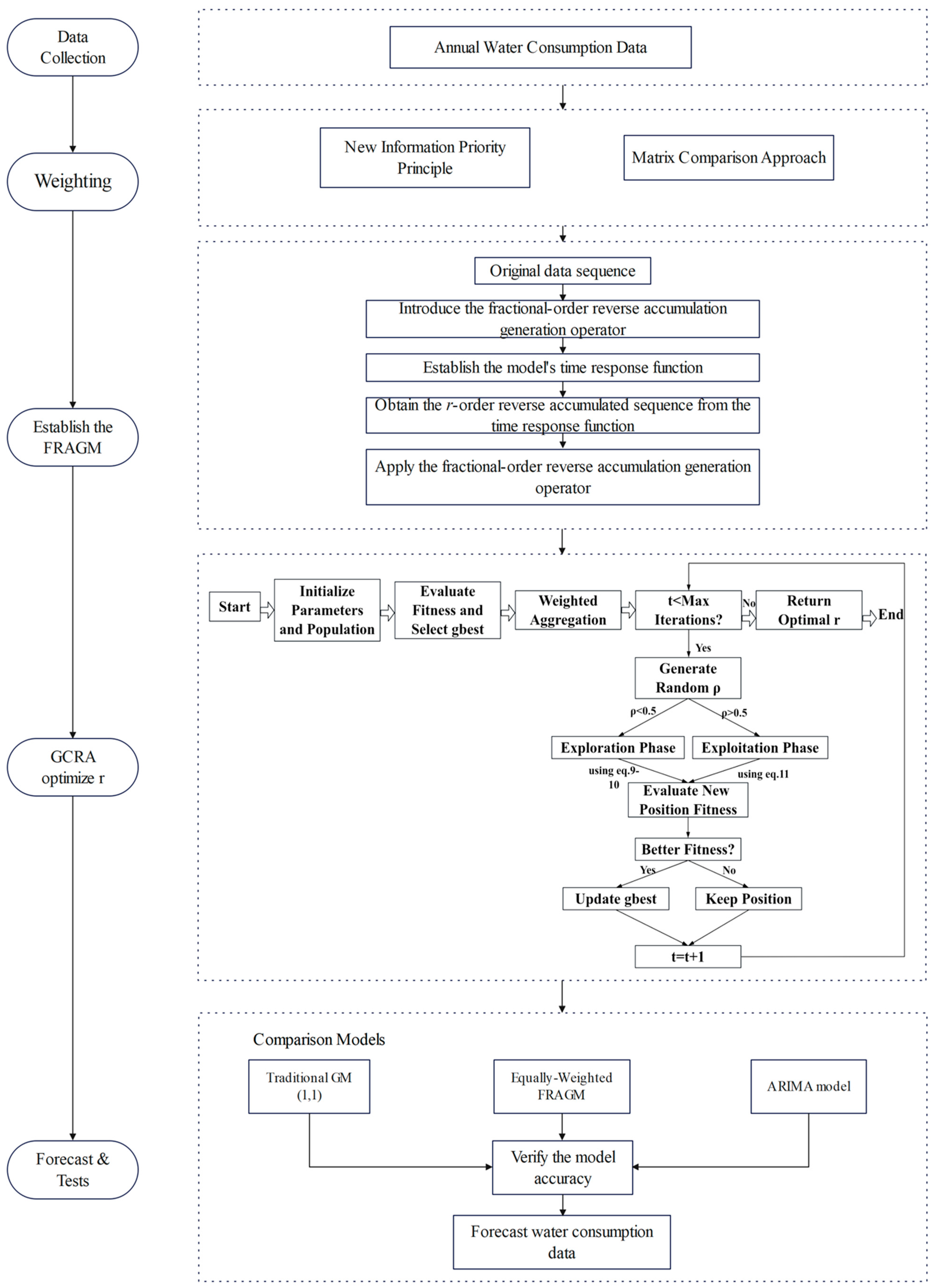
This section outlines the computational pipeline of the proposed forecasting framework, as visualized in Figure 1. The process begins by calculating yearly data weights based on the New Information Priority Principle, employing the Matrix Comparison Approach to assign higher weights to more recent years. The FRAGM is then formulated. This involves adopting reverse accumulation to prioritize recent data, introducing a fractional-order accumulation generation operator, and establishing a time response function to derive the prediction sequence. The fractional order r in FRAGM is optimized by the GCRA. The optimization aims to minimize the mean weighted relative error, where the weights in the error function are the yearly data weights previously obtained. Finally, the optimized model’s performance is compared against the traditional GM (1,1), the equally weighted FRAGM, and the ARIMA model, using consistent data preprocessing, train–test 4 splits, and evaluation metrics (MAE and MRE). The Diebold–Mariano (DM) test is applied to assess the statistical significance of performance differences.
Figure 1.
Technology framework.
3.1. Calculation of Yearly Data Weights Based on the New Information Priority Principle
To enhance the model’s responsiveness to recent data trends, we introduce the new information priority principle, assigning higher weights to more recent observations. This approach mitigates the interference of outdated patterns and better captures evolving water consumption behaviors, which is particularly crucial for cities undergoing rapid development or seasonal fluctuations.
According to the New Information Priority Principle, data closer to the present moment possess greater reference value and, therefore, warrant higher weights. Employing the Matrix Comparison Approach, a pairwise comparison of years is conducted to derive comparative judgments and ultimately determine each year’s weight. Specifically, a year judgment matrix is constructed by evaluating every possible year—pair, assigning a score of 1 to the more recent year and 0 to the earlier one, until all pairs have been assessed (see Li [] for the detailed procedure). Once the judgment matrix is complete, each year’s aggregate score is obtained by summing its row, and these scores are then normalized via Equation (1) to yield the final weights:
where is the total score of the k-th year, is the weight of the k-th year, and n is the total number of years in the dataset.
3.2. Model Formulation of the FRAGM
Reverse accumulation is adopted to prioritize recent data during sequence construction, which enhances the model’s sensitivity to the latest trends. For the original data sequence , the traditional integer-order accumulation generation operator (AGO) is defined as follows: . To enhance the model accuracy, the fractional-order reverse accumulation generation operator is introduced. Let denote the transformed sequence. Utilizing the Gamma function to extend the definition of factorial, the fractional-order reverse-accumulation generation operator can be expressed as follows:
where refers to the r-order reverse-accumulated result of the sequence, and k serves as the index for the water usage year.
The time response function serves as the core forecasting component, enabling future value prediction through parameter estimation. The time response function of the model is given by the following equation:
where is the r-order accumulated prediction sequence; the coefficients a and b can be determined by Equations (4) and (5):
where
Based on the time–response function, the r-order accumulated sequence is obtained, and the original prediction sequence is then recovered by applying the fractional-order reverse-accumulation operator.
3.3. GCRA-Based Optimization of the FRAGM
As a swarm intelligence optimization algorithm, GCRA is developed from the observation that greater cane rats adopt distinct collective foraging behaviors in breeding and non-breeding seasons. The algorithm dynamically balances global exploration and local exploitation by simulating dual-season foraging strategies []. The fractional order r significantly impacts the prediction performance. GCRA optimization adapts r to data fluctuations, minimizing prediction errors. This study employs GCRA to optimize the fractional-order r in the FRAGM. The mean weighted relative error between the predicted value and the actual value is selected as the objective function. The goal is to minimize the model’s prediction error through fractional-order optimization. A new information priority weighting is introduced into this formulation to ensure that data closer to the current time step receives greater emphasis during learning, thereby enhancing the model’s timeliness and prediction accuracy. The objective function incorporates weighted errors, ensuring recent prediction errors receive greater emphasis during optimization. The optimization purpose is captured in the following functional form:
GCRA iteratively searches for the optimal fractional order, maintaining an effective balance between exploration and exploitation. The detailed steps of the search process are outlined below:
- Step 1
Based on the parameter sensitivity analysis conducted in Section 5.3, set the algorithm parameters as follows: search agents N = 50, max iterations = 200, and fractional-order bounds rmin = 0, rmax = 2. Since the only variable being optimized is the fractional-order r, making the problem a one-dimensional optimization problem, the dimension is set to dim = 1. Initialize the population uniformly in [rmin, rmax]; each particle represents a candidate fractional-order ri. The fitness value f(ri) is evaluated for each agent using Equation (6). The candidate with the smallest fitness value is selected as the global best solution (gbest), referred to as the dominant male r.
- Step 2
After completing parameter initialization and boundary setting, each candidate fractional-order ri in the population is independently evaluated through the full FRAGM procedure to evaluate the fitness value defined by the objective function. Specifically, the ri-order fractional reverse-accumulated sequence is first constructed according to Equation (2). Subsequently, the model coefficients are estimated using the least-squares method described in Equations (4) and (5). Next, the time–response function in Equation (3) is applied to generate the fitted sequence, which is then inverse-accumulated to obtain the predicted values . Finally, the fitness value f(ri) of each individual is calculated using the objective function f(r). Following the “smaller error is better” principle, the individual with the minimum fitness is selected as the current global best position gbest, and its fitness value Fgbest is recorded. This result serves as the core reference for the subsequent initial aggregation step and the main iteration process.
- Step 3
To improve sample efficiency in the one-dimensional fractional-order search problem, after the initial gbest has been determined, we introduce a weighted aggregation step. This step moves some or all agents toward gbest along the already identified promising region, thereby concentrating subsequent computational effort in more promising subspaces during later iterations. The weighted aggregation formula based on gbest is given as follows:
in Equation (8), xi denotes the current solution of individual i (a scalar fractional order in this study), and the coefficient w ∈ (0, 1] controls the aggregation strength. According to the study by Agushaka et al. [], setting w = 0.7 achieves a balanced trade-off between maintaining diversity and realizing effective aggregation and thus can be adopted as the default value.
- Step 4
During each iteration, the algorithm enters either the exploration phase or the exploitation phase according to the value of variable ρ. The value of ρ, which balances exploration and exploitation based on a probabilistic rule, is finally finely tuned to 0.5, as verified by Agushaka et al. [] through parameter tuning—this value enables GCRA to achieve an optimal balance between exploration and exploitation. If ρ < 0.5, the population enters the exploration phase; otherwise, it enters the exploitation phase.
Within the exploration phase, the updated positions of the rat population are computed according to the dominant male’s position, as illustrated in Equation (9). When an individual achieves a better objective function value than the current optimum, the optimum is replaced, and other individuals update their positions relative to it; if not, the individual moves away from the optimum position. Furthermore, greater cane rats relocate only when the objective function value at the candidate position is superior; otherwise, they will maintain their previous position. This strategy is modeled as shown in Equation (10):
where Xi denotes the next state or new state of greater cane rat; xk is the dominant male position; xi is the current position; f(xi) denotes the fitness value of the dominant male; represents the evaluation result of the current candidate. The parameter C is a random variable in the search space, included to emulate scattered food and shelter. Parameters rfood, α, and β are derived from references [].
In exploitation phase, a female individual m (m ≠ k) is randomly selected, and the new position is computed according to the following Equation (11):
where μ is a stochastic parameter that assumes integer values between 1 and 4, representing the number of offspring.
If the new position improves fitness, it replaces the old one; otherwise, the original position is retained.
- Step 5
After each iteration, the fitness values are recalculated. If a superior solution is discovered, gbest is replaced accordingly; the iterations proceed until convergence or until the predefined maximum is met.
- Step 6
The final gbest is returned as the optimized fractional-order r, which minimizes the weighted prediction error of the FRAGM.
3.4. Comparison Models
To assess its effectiveness, the proposed approach is evaluated in comparison with two standard grey prediction models, namely the equally weighted fractional-order reverse accumulation model, the traditional GM (1,1), and the ARIMA model.
- (1)
- Traditional GM (1,1)
The GM (1,1) model originates from grey system theory and is suitable for situations with insufficient information and small sample sizes. This approach applies first-order accumulation generation to raw data, producing a smoothed sequence that mitigates stochastic fluctuations. Its core principle involves modeling the accumulated data sequence to extract inherent trends, which subsequently inform future predictions.
- (2)
- Equally Weighted FRAGM
The equally weighted FRAGM differs from the model in this paper only in that the weights in Equation (5) are equal. All other aspects are identical to the model in this paper.
- (3)
- ARIMA model
As a classical linear baseline for time-series forecasting, the ARIMA model uses an autoregressive (AR) component to capture correlations with past values, an integrated (I) component to render the sequence approximately stationary, and a moving-average (MA) component to model serially correlated shocks in residuals. Its orders are determined by minimizing the Akaike Information Criterion (AIC) over a candidate grid (p = 0–3, d = 0–1, q = 0–3), parameters are estimated via likelihood-based methods, and multi-step forecasts are generated iteratively from the fitted model.
To ensure a fair comparison, the GM (1,1) model, the equally weighted FRAGM, the proposed FRAGM, and the ARIMA model all adopted identical data-preprocessing procedures, the same training/testing split, and the same evaluation metrics (MAE, MRE), thereby maintaining consistency across the comparison framework.
3.5. Comparing Metrics
Currently, the prediction accuracy of models is evaluated using a range of error metrics, among which mean absolute error (MAE) and mean relative error (MRE) are widely applied []. Different studies select one or more of these methods. Typically, the model that minimizes error under a chosen criterion is considered the most accurate. Here, MAE and MRE are selected as the assessment measures, and the expression for MAE is given in Equation (12).
The calculation of the MRE is shown in Equation (13):
The evaluation criteria for MRE follow Wang’s definition [], as detailed in Table 1:
Table 1.
MRE evaluation criteria.
These evaluation metrics offer a comprehensive measure of the model’s performance, reflecting its accuracy from multiple perspectives.
3.6. Model Performance Assessment Methods
To measure the predictive performance of the models, Diebold and Mariano proposed the DM statistic for model performance testing. The DM test is primarily used to compare two competing models []. Let the time series be , the forecast values from the two models be , and the corresponding forecast errors be :
In general, the loss function of each model at time t depends on both the actual and forecast values, denoted as . Since the loss function is a function of the forecast error, it can also be expressed as . If the two models have equal predictive performance, the expected values of their loss functions should be identical:
where the value of E(dt) < 0 indicates that Model 2 outperforms Model 1, while the value of E(dt) > 0 suggests that Model 1 is superior. The DM statistic is constructed as follows:
where is the indicator function, and denotes the rank of the absolute differences in loss functions between the two models, ordered from smallest to largest. T represents the total sample size. The DM statistic follows a standard normal distribution. In this paper, the MRE is adopted as the loss function for the DM test.
4. Case Study
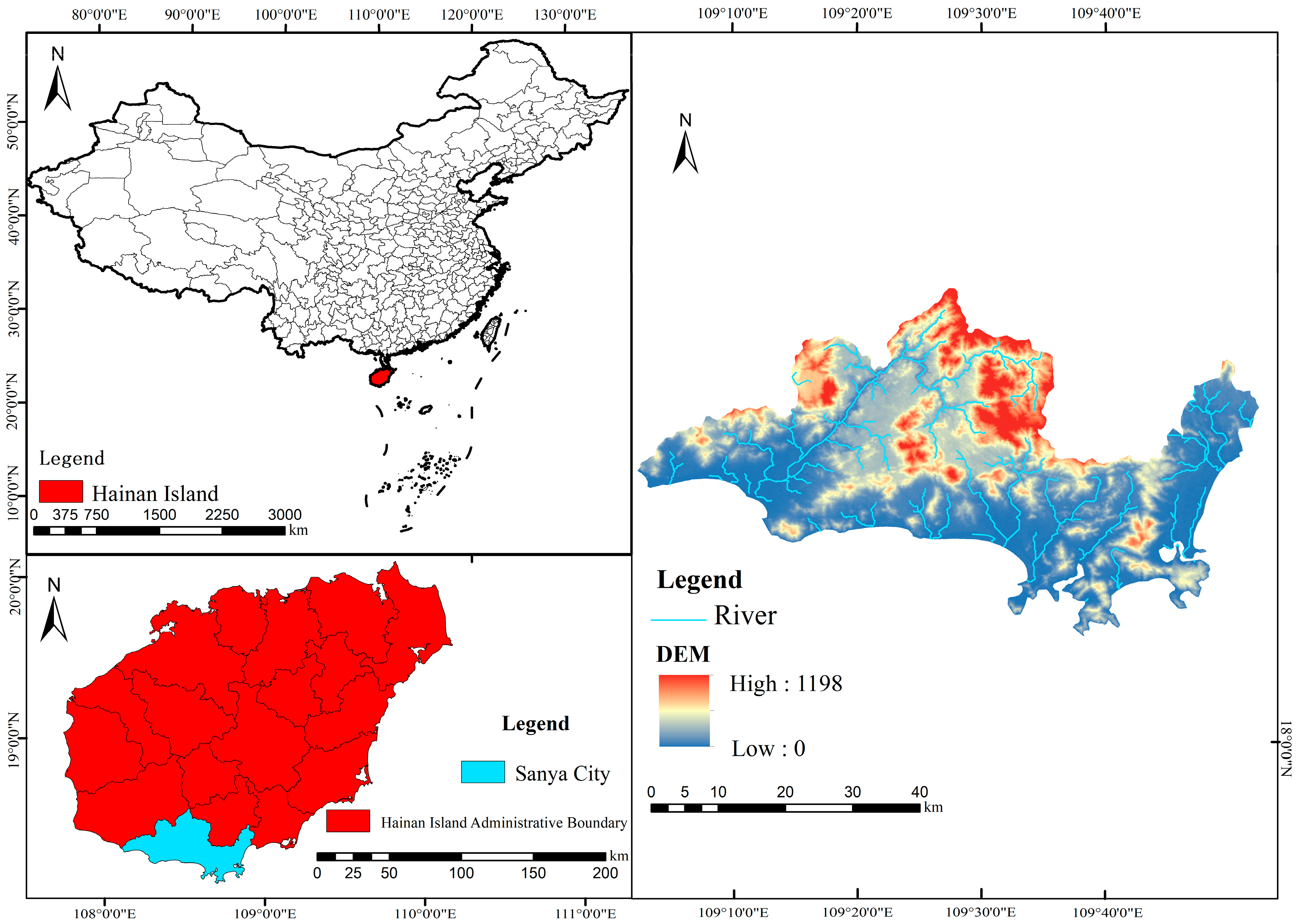
This paper selects Sanya City, Hainan Province (18°09′–18°37′ N, 108°56′–109°48′ E) as the study area (see Figure 2). Located at the southernmost tip of Hainan Island, Sanya possesses abundant natural resources and a unique ecological environment, ranking among China’s most renowned tourist destinations. Following the announcement of the Master Plan for the Construction of the Hainan Free Trade Port, tourism in Sanya has developed rapidly, becoming a critical economic pillar. The vigorous expansion of tourism has significantly increased local water demand and consumption. The Free Trade Port construction has spurred rapid economic growth, while industrial development further escalates water requirements. With rising marginal costs of water resource development, water scarcity and aquatic ecosystem degradation have emerged as bottlenecks constraining urban progress. According to the Sanya Statistical Bulletin, the city’s permanent population remains relatively small, reaching approximately 1.106 million residents by the end of 2023. In sharp contrast, the tourism influx is remarkably large in 2023; Sanya received a total of 25.71 million overnight visitors, representing a 95.56% increase compared with the previous year and a 7.75% growth over 2019 under the same statistical standard. This indicates that during peak tourist seasons, the number of visitors entering the city within a short period can be dozens or even hundreds of times greater than the resident population, creating pronounced seasonal fluctuations and peak shocks in urban water demand. Consequently, predicting Sanya’s water consumption is essential to inform integrated water supply planning.
Figure 2.
Location map of the research area.
5. Model Application and Results
5.1. Data Preprocessing
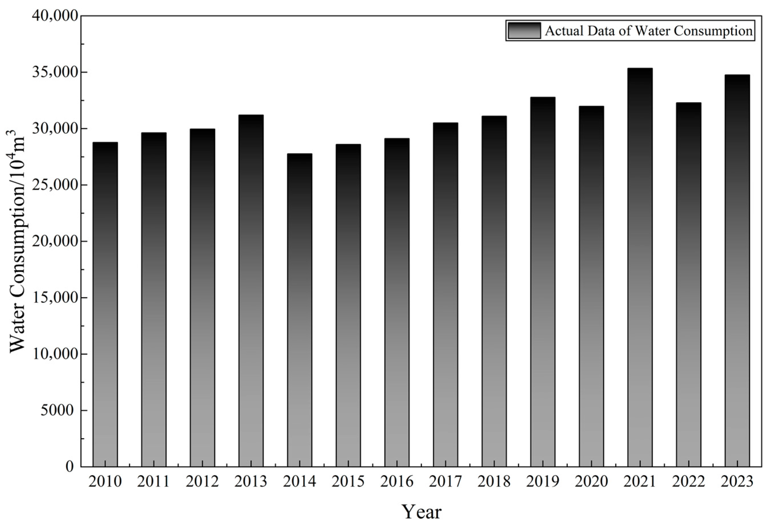
To validate the model, the total water consumption data of Sanya City from 2010 to 2023 were adopted as a case study. The measured data are illustrated in Figure 3. It is noteworthy that in time series modeling, missing data or temporal discontinuities can significantly compromise model stability and prediction accuracy. When such issues arise, it is essential to determine the missingness mechanism and apply appropriate imputation methods—such as interpolation, moving average, Kalman smoothing, or model-based approaches—to preserve temporal consistency and statistical characteristics []. The dataset used in this study is complete and temporally continuous, with no missing or inconsistent records, thereby ensuring the reliability of subsequent modeling analyses.
Figure 3.
Annual total water consumption in Sanya City (2010–2023). Unit: 104 m3.
This study adopts the rolling-origin-recalibration scheme to evaluate forecasting performance. Under this scheme, the forecast origin is shifted forward step by step; at each new origin, the model parameters are re-estimated on all available observations up to that point, after which a one-step-ahead forecast is produced and the prediction error recorded. Specifically, the model is first fitted on the initial training block (2010–2020) to forecast 2021; the training set is then extended to 2010–2021, the parameters are re-estimated on this expanded dataset, and the forecast for 2022 is generated; the procedure continues in the same manner. All comparison methods follow the same recalibration process, with model parameters re-estimated at each iteration. This design ensures comparability across models and simulates an operational workflow, in which retraining occurs as new observations become available. Rolling-origin-recalibration not only compensates for the shortcomings of insufficient data but also enables models to adapt to potential dynamic changes in the data.
5.2. Algorithm Performance Evaluation
Evaluating and contrasting the performance of intelligent algorithms is central to algorithm optimization research and informs the choice of tools for complex computational challenges. This study compares GCRA with PSO.
The parameters were set as follows: population size N = 100, dimension dim = 50. Four standard test functions are used to test the above-mentioned algorithms, and detailed information of the test functions is shown in Table 2 [,].
Table 2.
Test functions.
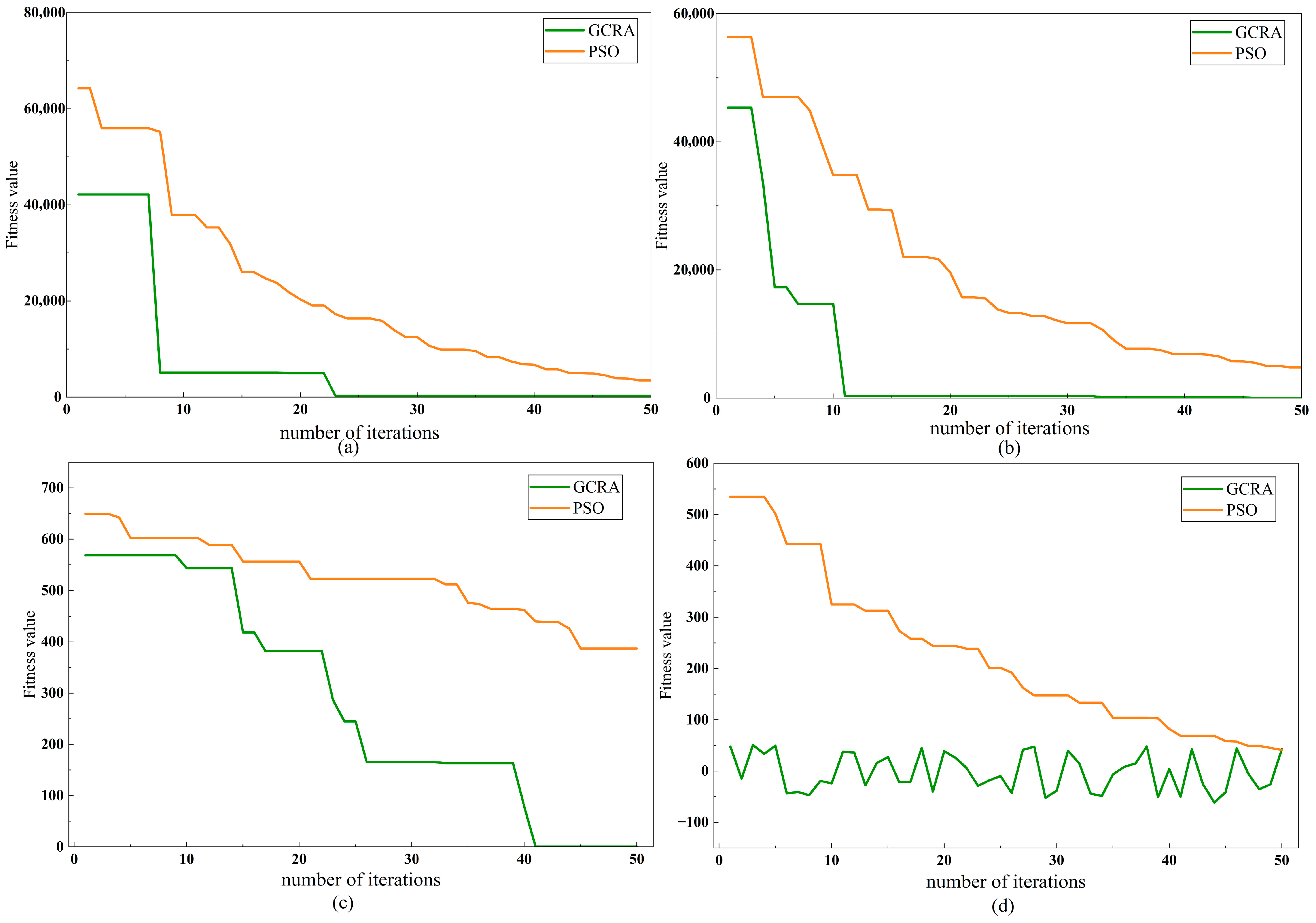
Performance tests were conducted for each algorithm based on the above parameter settings. To reduce the impact of randomness on the experiment, each algorithm was iterated 50 times. In-depth investigations were performed on their convergence characteristics and variations in fitness values to identify performance distinctions between the algorithms and to inform their selection for FRAGM applications. Figure 4 illustrates the convergence paths of different algorithms when applied to the test functions.
Figure 4.
Convergence curves of GCRA and PSO on each test function: (a) F1; (b) F2; (c) F3; (d) F4.
The experimental evaluation, summarized in Table 2 and Figure 3, involved tests on unimodal functions F1 and F2 as well as multimodal functions F3 and F4.
In the unimodal function tests, GCRA exhibits a significantly faster convergence rate. In the F1 test, GCRA demonstrates remarkably efficient convergence: its fitness value experiences a sharp decline at iteration t = 7 and stabilizes at the global best value by t = 22. In contrast, although the convergence process of the PSO algorithm shows an obvious inflection point, its fitness curve decreases gently and fails to reach a stable state within the maximum number of iterations. Similarly, in the F2 test, GCRA once again demonstrates the advantage of rapid convergence, with its convergence curve showing a consistent pattern to that in F1. The fitness value quickly approaches the theoretical optimal solution in the early stages of iteration, while the convergence speed of PSO lags significantly. This can be attributed to the fact that GCRA directly guides the population through the global best and efficiently exploits the unique optimal region of unimodal functions by combining multi-strategy position update mechanisms, whereas PSO exhibits obvious convergence delay due to its reliance on gradual information transmission between particles.
In multimodal function tests, GCRA demonstrates even more prominent advantages. For the F3 function, which exhibits dense local optima due to oscillations of the cosine term, GCRA achieves stable convergence by avoiding entrapment in local optima through continuous exploration via probabilistic strategy switching and multi-dimensional perturbations. In contrast, the PSO algorithm, influenced by particle movements dominated by the global best, reinforces local solutions, resulting in convergence to suboptimal values ultimately. In the F4 test, where the product term leads to minimal differences in fitness between local optima and the global optimum, GCRA continuously approaches the global optimum through its iterative position correction mechanism. PSO, however, lacks proactive exploration capability; although its curve remains stable, it fails to distinguish between the global best and local best, leading to insufficient convergence accuracy.
The experimental findings indicate that GCRA outperforms PSO in terms of both optimization ability and convergence behavior. This conclusion provides a theoretical basis for the selection of the fractional-order optimization algorithm in this study.
5.3. Parameter Sensitivity Analysis
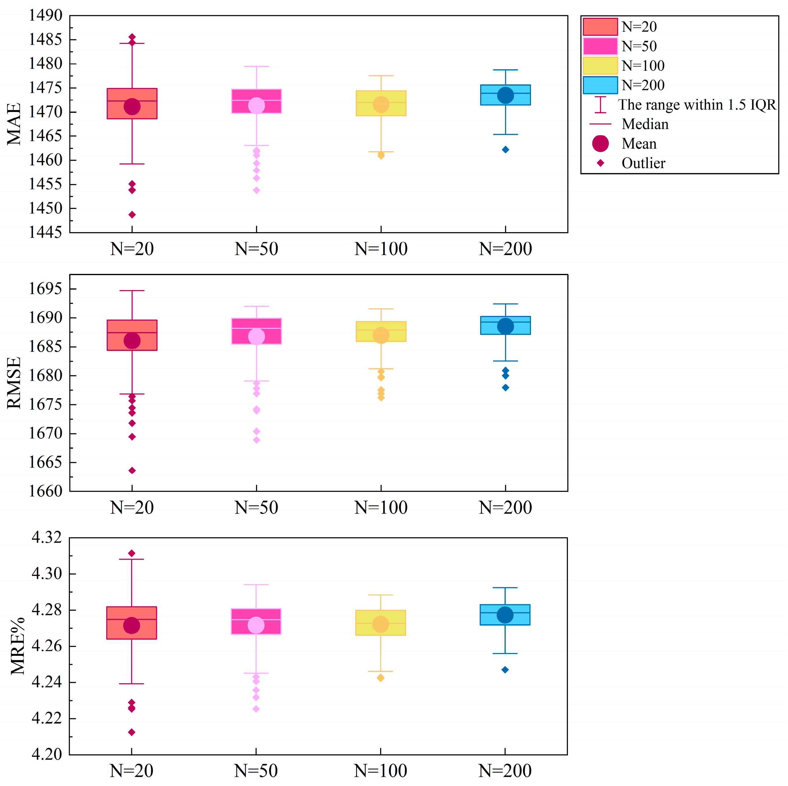
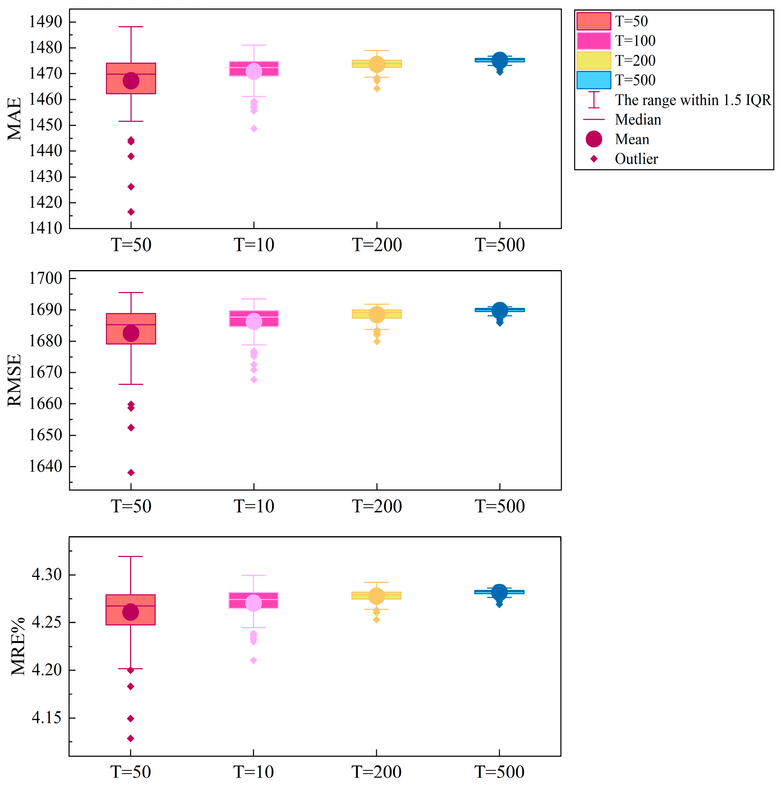
To further investigate the robustness of the proposed FRAGM with GCRA optimization, a parameter sensitivity analysis was conducted. Three key parameters of the GCRA were selected for evaluation: the population size , the maximum number of iterations , and the fractional order . Following the principle of one-factor-at-a-time design, each parameter was varied across predefined ranges, while the other two were fixed at their default values (N = 50, T = 100, r = 1.0). Specifically, the tested values were N = [20, 50, 100, 200], T = [50, 100, 200, 500] and r = [0.5, 1.0, 1.5, 2.0].
For each parameter configuration, a rolling-origin-recalibration forecasting procedure (2010–2020 as training, 2021–2023 as testing, stepwise expansion) was performed 100 times to account for the stochasticity of the GCRA. Performance was assessed using three error metrics: MAE, MRE, and root mean square error (RMSE). The resulting error distributions were visualized by boxplots, allowing for a direct comparison of parameter impacts. The results are shown in Figure 5, Figure 6 and Figure 7.
Figure 5.
Sensitivity analysis of parameter N.
Figure 6.
Sensitivity analysis of parameter T.
Figure 7.
Sensitivity analysis of parameter r.
The results indicate that the model is relatively insensitive to N; when N > 50, the MRE stabilizes at approximately 4.26–4.29, with little benefit from further enlarging the population size. Increasing T yields moderate improvements: with fewer than 100 iterations, the error remains slightly higher, whereas performance converges when T = 200, and further increases bring only marginal gains. In accordance with subsequent experiments, this paper sets N = 50 and T = 200 to strike a balance between computational efficiency and predictive accuracy. By contrast, the fractional order is highly sensitive, with MRE ranging dramatically from about 5.24 to over 90 depending on its value. Large values of substantially deteriorate accuracy, underscoring the necessity of employing GCRA’s optimization mechanism to adjust this parameter. Overall, the sensitivity analysis confirms that the FRAGM–GCRA framework achieves a robust balance between accuracy and efficiency under appropriate parameter configurations, highlighting its reliability and practical applicability.
5.4. Optimal Order Determination via GCRA
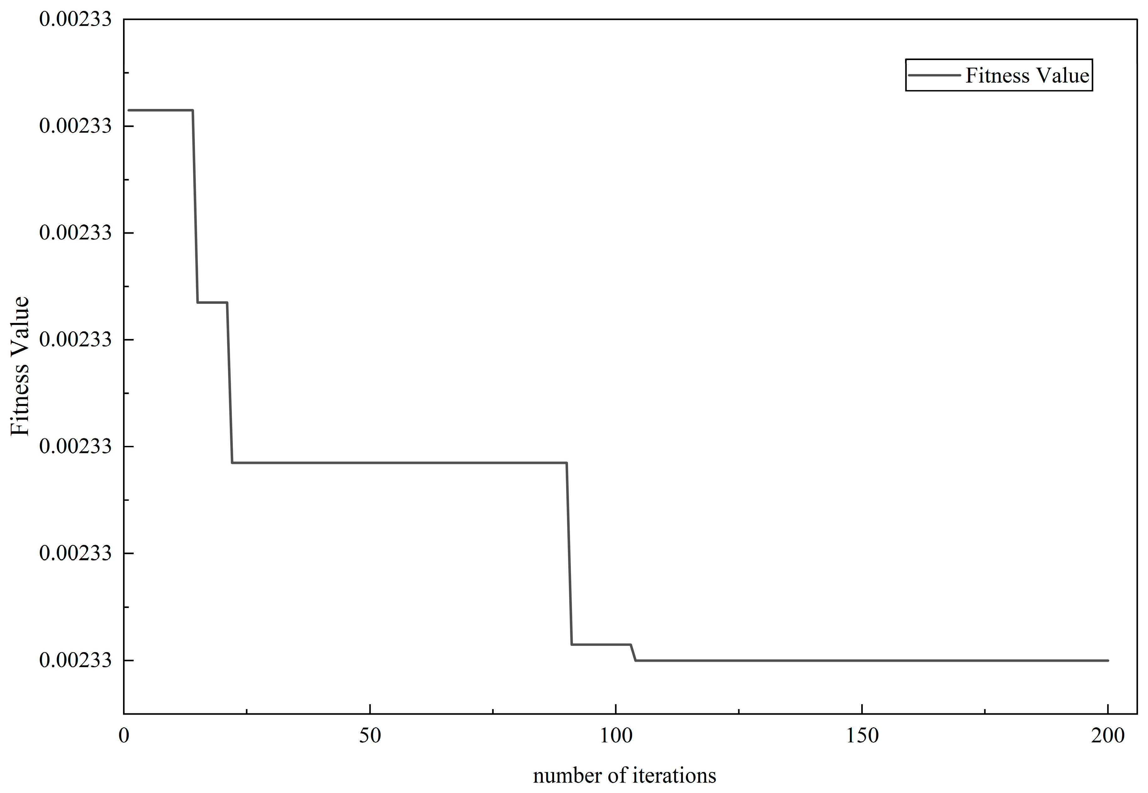
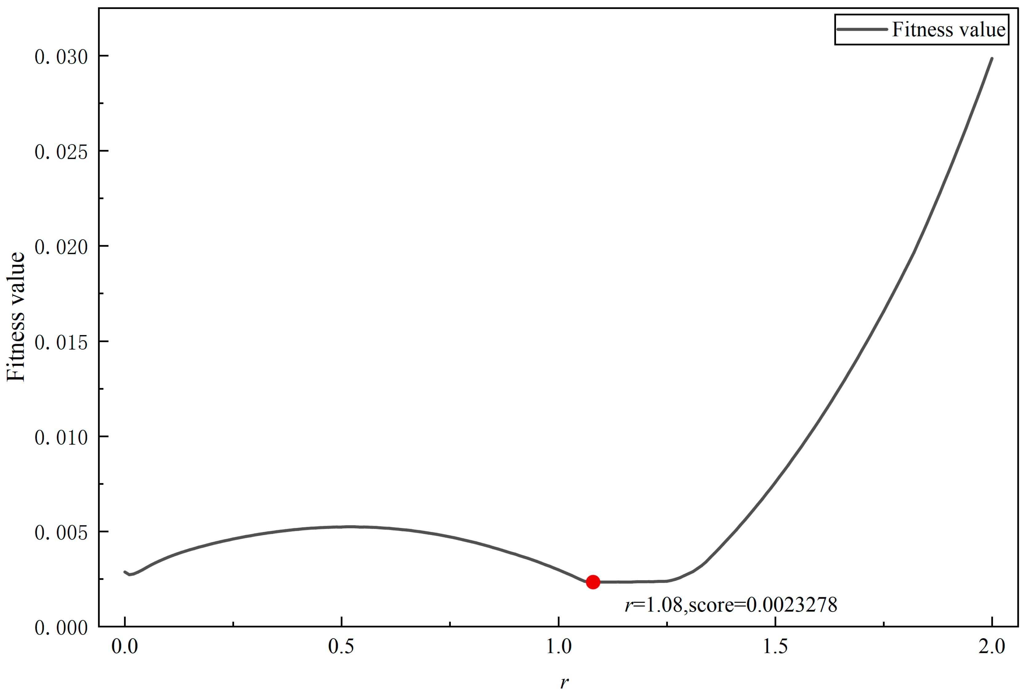
By optimizing the weighted average error of the FRAGM using the GCRA, the optimal fractional-order r of the model was determined. Both the optimization process and the numerical solution of the model were implemented programmatically in MATLAB R2018b to ensure computational reproducibility and accuracy. The iteration process of the objective function, illustrating the variation in fitness values, is shown in Figure 8. When GCRA meets the termination criterion, the corresponding fractional order r is taken as the optimal parameter for FRAGM. The reported r in Figure 9 is the best value obtained.
Figure 8.
Evolution of the fitness function value with iteration count.
Figure 9.
Variation in the fitness function value with r.
In the initial iteration stage, the fitness function did not fluctuate. As iterations proceeded, when the number of iterations reached t = 14, the fitness values converged rapidly, and finally completed convergence at t = 104, indicating that the optimal solution had been successfully identified. At this stage, the output gbest corresponds to the optimal order.
5.5. Analysis of Training and Testing Set Prediction Results
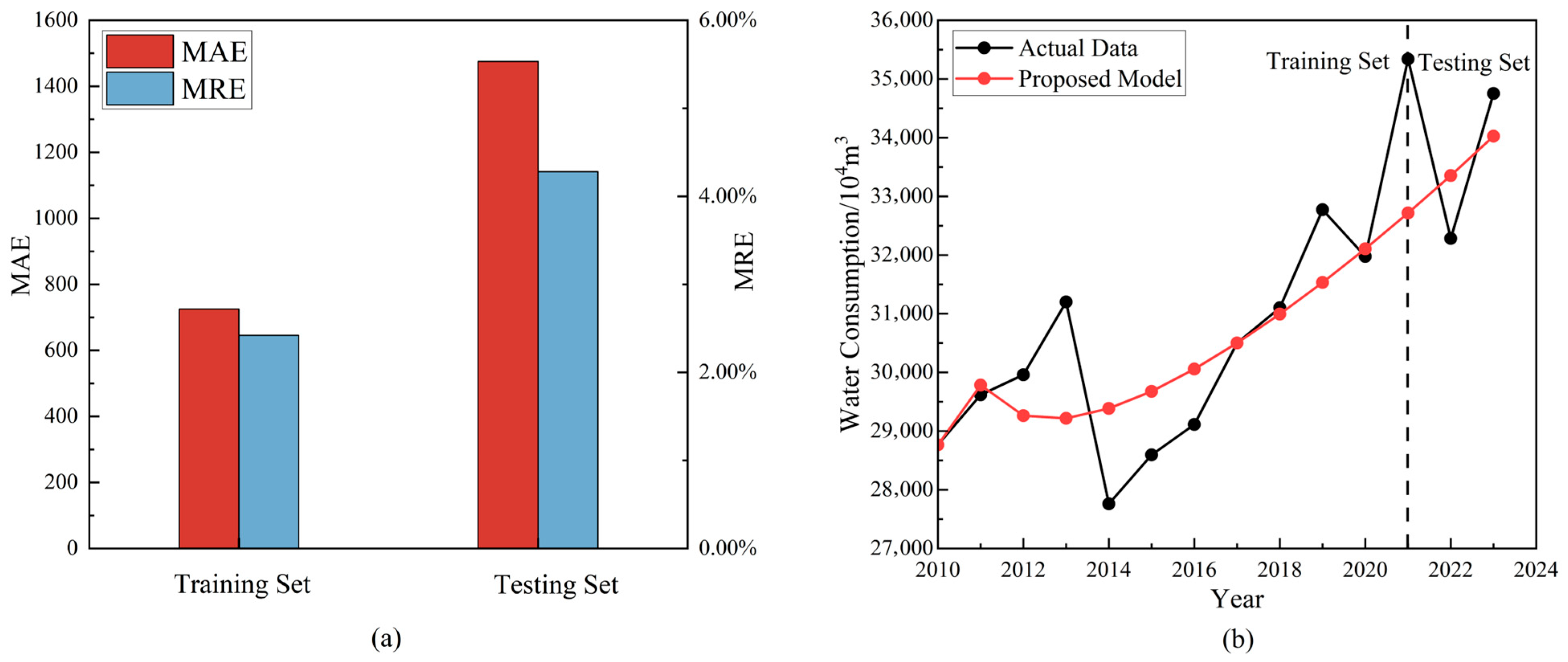
The proposed model uses the rolling-origin-recalibration scheme, taking data from 2010 to 2020 as the initial training set, and the forecast origin is shifted stepwise for forecasting. Prediction performance is evaluated by calculating MAE and MRE. Detailed results are presented in Figure 10.
Figure 10.
Prediction performance of the proposed model: (a) error metrics comparison between training and testing sets; (b) comparison of simulated results with actual water consumption.
Findings show that, on the training set, the proposed model yields an MAE of 724.89 and an MRE of 2.42%. For the testing set, the MAE is 1475.33 with the MRE of 4.28%. Both training and testing MRE values fall below the 5% excellence threshold specified in Table 1, indicating exceptional predictive performance. This confirms the model’s applicability for water consumption forecasting in tropical island tourist cities.
5.6. Model Comparison and Validation
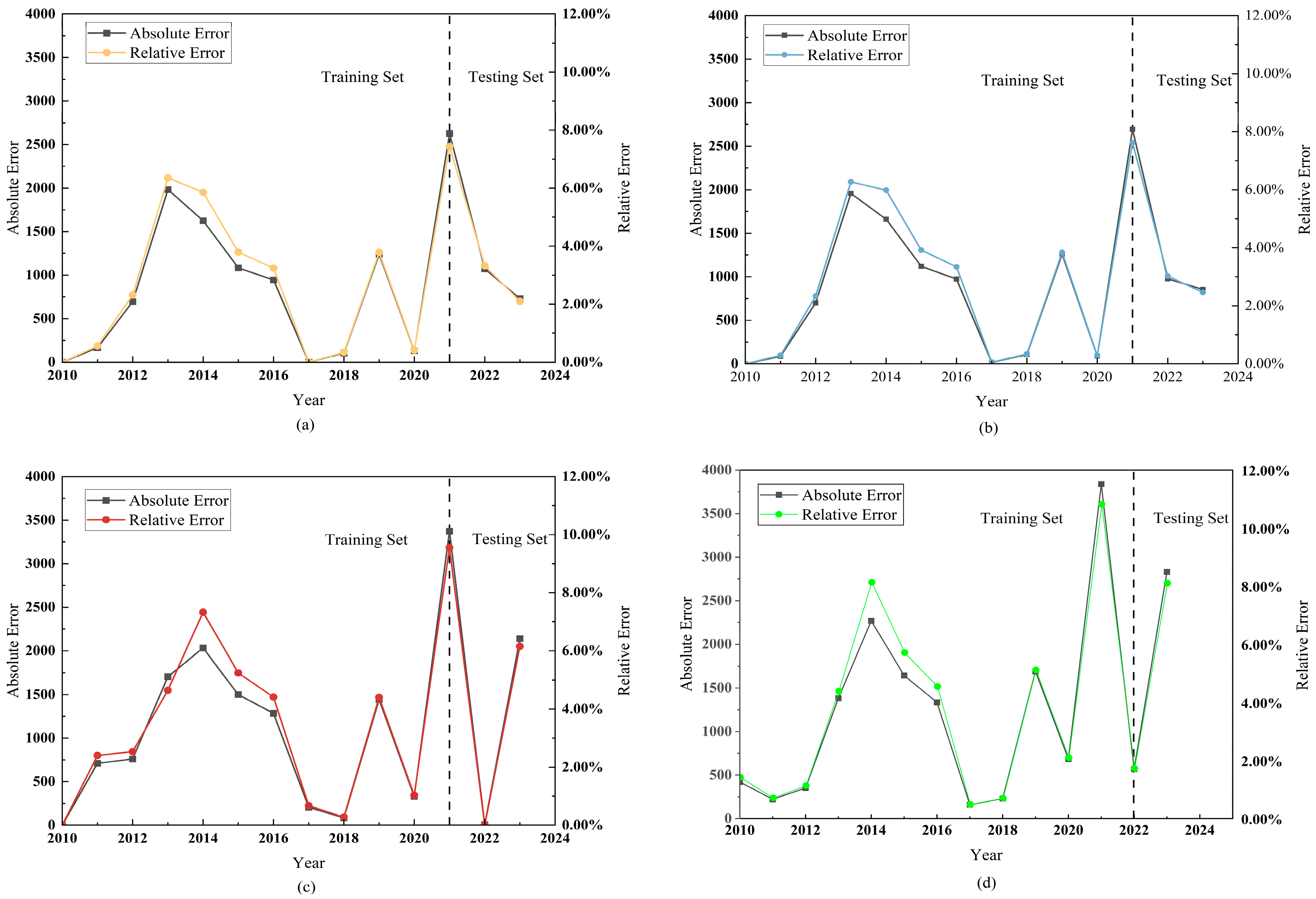
To further validate the performance of the proposed model, compared its error metrics against those of the ARIMA model, GM (1,1), and the equally weighted FRAGM. Results are presented in Figure 11.
Figure 11.
Error comparison of simulation and prediction among different models. (a) Proposed model; (b) equally weighted FRAGM; (c) GM (1,1); (d) ARIMA model.
For the 2010–2015 simulation period, the equally weighted model achieved an MRE of 3.13%, while the proposed model yielded 3.15%. The equally weighted model thus demonstrated slightly better fitting for historical data. During 2016–2020, the equally weighted model’s MRE was 1.57%, whereas the proposed model’s MRE reduced to 1.55%. This reversal occurs because, starting in 2016, the weights assigned by the proposed model exceeded the fixed weights of the equally weighted model for the first time. This indicates greater emphasis on 2016–2020 data by the proposed model, contrasting with its lower weighting of 2010–2015 data. For recent data with higher weights, the proposed model fully assimilates information, resulting in smaller errors than the equally weighted model. Conversely, for older data with reduced weights, it deliberately minimizes learning to prevent overfitting to noise from inconsistent data, leading to slightly larger simulation errors for such data. On the testing set (2021–2023), the proposed model achieved an MAE of 1475.33 and an MRE of 4.28%—both lower than the equally weighted model. This testing-set-prediction superiority arises because the model not only deliberately limits learning from older periods by reducing the weighting of historical data—thereby avoiding the assimilation of noise caused by inconsistencies—but also places greater emphasis on recent observations by increasing the weight of newer data. This dual focus, which mitigates overreliance on outdated information while prioritizing learning from the latest patterns, is key to enhancing prediction accuracy.
The ARIMA model demonstrates significantly larger prediction errors on both the training and testing sets compared to the proposed model. Specifically, it yields an MAE of 944.6662 and an MRE of 3.17% on the training set, while on the testing set, these values rise to 2412.9319 and 6.92%, respectively. This pronounced performance gap can be attributed to the model’s limited adaptability to the specific data characteristics. ARIMA models generally perform best with relatively stable and linear time series. However, the water consumption data in Sanya City, influenced by its tourism-driven economy, exhibits substantial fluctuations and nonlinear trends. As a result, the ARIMA framework shows poor adaptability to such dynamic, small-sample conditions, leading to a noticeable decline in predictive accuracy on the testing set.
The GM (1,1) achieved an MAE of 914.2 and an MRE of 3.07% on the training set and an MAE of 1839.43 with MRE of 5.24% on the testing set. Although the GM (1,1) avoids overlearning of older training data (its MRE for 2010–2015 simulation was 3.83%, larger than the proposed model’s), it also fails to sufficiently learn recent training data (its MRE for 2016–2020 simulation was 2.16%, larger than the proposed model’s). This indicates the traditional model’s inability to fully assimilate new information, constituting one primary reason for its poor prediction performance. Additionally, the integer-order limitation and absence of reverse accumulation mechanics further degrade its forecasting efficacy. To provide a statistical assessment of predictive superiority, the DM test was applied using the MRE as the loss function. The comparison uses 13 comparable forecast error observations for each model pair. The DM statistic for the proposed model versus the traditional GM (1,1) is −2.20, with a two-tailed p-value of 0.0277, indicating that the proposed model’s forecasts are significantly more accurate than those of GM (1,1) at the 5% significance level, which is consistent with the above discussion.
5.7. External Validity Verification
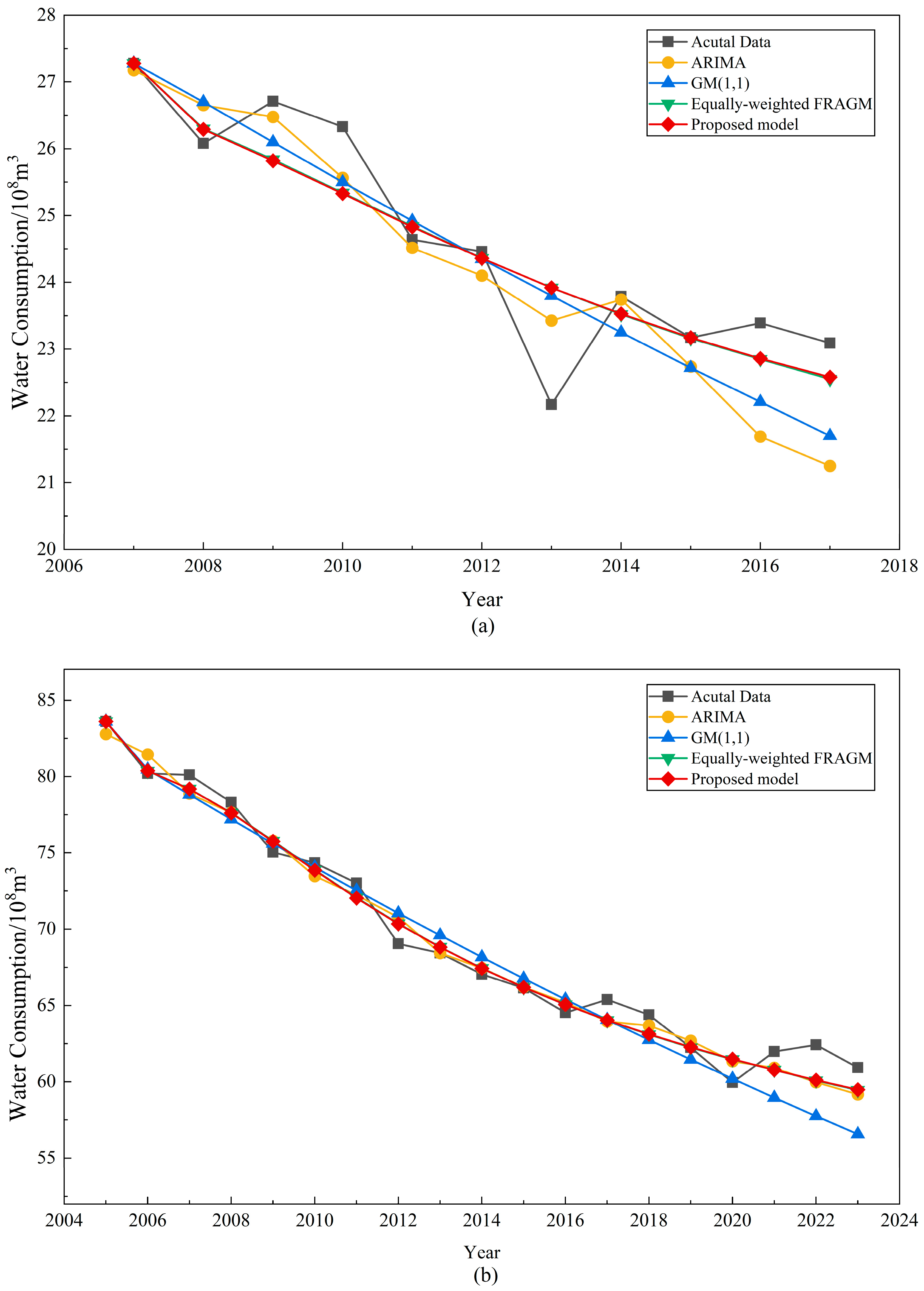
To further examine the external applicability of the model, the modeling and evaluation procedures were extended to two cities with distinct characteristics: Guangzhou and Tongliao. The water consumption data of Guangzhou and Tongliao were obtained from the local water resources bulletins. Guangzhou represents a large southern metropolis with a longer sample period, greater economic scale, and more complex influencing factors; Tongliao, by contrast, represents a smaller city with a shorter sample period and markedly different climatic and socio-economic conditions. By validating model performance across such heterogeneous series, this study aims to assess the robustness of the proposed method under varying sample lengths and urban contexts, thereby enhancing the generalizability and practical relevance of the conclusions. The specific implementation details are consistent with other parts of this study, and the forecasting results of the models are shown in Figure 12.
Figure 12.
Comparison of prediction effect of each model: (a) Tongliao; (b) Guangzhou.
In the validation representing northern medium–small cities, the improved FRAGM demonstrated excellent adaptability in Tongliao City. The MRE on the testing set was 2.24%, showing significantly superior accuracy compared to the benchmark models. Specifically, the improved FRAGM reduced the error by 0.08 percentage points compared to the equally weighted version (2.32%), reflecting the effectiveness of the new information priority mechanism in predicting water consumption in small- and medium-sized cities. The traditional models performed poorly in this case: the GM (1,1) model had an error of 5.53%, indicating its limited ability to capture the data characteristics of such cities; the ARIMA model recorded a high error of 7.62%, revealing the significant limitations of linear methods in handling the seasonal water usage patterns of northern cities.
Validation in the southern megacity of Guangzhou further confirmed the applicability of the improved FRAGM. The model achieved an MRE of 2.67% on the testing set, maintaining the best performance. Although the accuracy improvement over the equally weighted model (2.71%) was only 0.04 percentage points, given Guangzhou’s annual water consumption scale of billions of tons, this improvement corresponds to an optimization potential of millions of tons of actual water volume. Notably, the traditional GM (1,1) model had an error of 6.51% in this case, reflecting its inadequacy in the complex water usage systems of megacities; although the ARIMA model achieved a relatively better result of 2.84%, it still could not match the comprehensive performance of the improved FRAGM.
Through systematic validation in three distinct Chinese cities—the tropical tourist city of Sanya, the southern megacity of Guangzhou, and the northern medium–small city of Tongliao—the improved FRAGM has demonstrated superior and stable prediction performance. This cross-regional, multi-type empirical testing provides strong evidence that the model maintains excellent adaptability when confronted with diverse urban characteristics and hydrological conditions. Although the numerical improvement compared to the equally weighted fractional-order reverse accumulation model is modest, the proposed model performs significantly better in terms of prediction volatility and output stability. The reduced prediction variance resulting from this stability makes the forecasts more trustworthy for water supply management authorities; furthermore, it is crucial to emphasize that a 0.1% error may correspond to a difference of millions of tons of water at the scale of a city’s total water consumption; this minor yet consistent error improvement translates directly into lower dispatch costs and higher operational efficiency. The multi-case validation strategy effectively enhances the external validity of this research.
6. Discussion
The key contribution of this study lies in the enhanced forecasting accuracy of the proposed model compared to benchmark models. The precise predictions enable water utilities to optimize urban water allocation schemes, facilitating highly efficient utilization of water resources and effectively reducing water waste from over-supply. This improvement not only conserves valuable water resources but also provides crucial support for sustainable urban water management.
The primary practical value of our model lies in its superior prediction accuracy over existing alternatives. For water managers, this enhanced precision directly translates to more reliable estimates for water demand. Consequently, they can plan daily allocation and reservoir storage with greater confidence, effectively mitigating the risks of both water wastage and supply shortages. This reliability is fundamental to optimizing the utilization of existing water infrastructure and forms a critical data foundation for any subsequent sustainable management strategy.
While affirming the value of the model, it is also necessary to carefully evaluate its potential validity threats. In terms of external validity, the representativeness of the case cities may affect the generalizability of the conclusions. To address this, this study selected three cities—Sanya, Guangzhou, and Tongliao—with significant differences in geographical and developmental characteristics. This multi-case design effectively enhances the generalizability of the research findings. Regarding internal validity, this study adopted a rolling-origin-recalibration scheme to ensure all models were compared under equivalent conditions, while parameters were optimized using the GCRA to minimize human-induced bias. For construct validity, multiple metrics, including MRE and MAE, were employed to ensure the comprehensiveness of model evaluation.
While multifactor time series models can effectively identify relationships between dependent and independent variables, this approach significantly increases data requirements. Moreover, numerous factors drive water consumption, and not all relevant factors have been fully identified or quantified. Additionally, there is currently no standardized method for selecting which variables should be used as predictors. For these reasons, this study employs the improved FRAGM within a univariate forecasting framework, extracting patterns solely from the water consumption sequence itself. This approach not only demonstrates the model’s capability in handling small-sample data but also aligns with the reality of often incomplete information in water management practice []. Future research will explore the incorporation of key exogenous factors through multivariate grey models or hybrid modeling approaches, aiming to enhance predictive performance while maintaining the model’s applicability across diverse urban contexts.
Ultimately, the model provides more than just a technical forecasting tool; more importantly, it supports the transition toward sustainable resource governance by integrating predictive analytics with ecological protection, equitable water access, and urban system resilience amid uncertainty. By systematically identifying and mitigating various validity threats, this study ensures the scientific rigor and reliability of its conclusions, thereby providing robust support for sustainable water resource management in cities with diverse characteristics.
7. Conclusions
(1) This study proposes an improved FRAGM that quantitatively integrates the new information priority principle during model construction. Through the matrix comparison method, higher weights are assigned to recent data, resolving the grey model limitations in learning historical data. This mechanism enables the model to more effectively capture emerging trends in the data evolution. Furthermore, extending the conventional first-order accumulation to fractional-order reverse accumulation significantly enhances predictive capability. The optimized model was applied to forecast water consumption in Sanya City, with experimental results demonstrating substantial improvements in prediction accuracy and adaptability.
(2) To evaluate the model performance, the proposed model was compared against the GM (1,1), the equally weighted FRAGM, and the ARIMA model. Results demonstrate that both the GM (1,1) and ARIMA exhibit poorer performance in testing-set prediction. The deficiency of GM (1,1) stems from its integer-order formulation, forward accumulation mechanism, and undifferentiated learning approach. The ARIMA model, while achieving a lower training error, shows a significantly higher testing error, indicating its poor adaptability to small-sample water consumption data in tropical island cities due to its linearity and stationarity assumptions. Relative to the proposed model, the equally weighted model assigns higher weights to the 2010–2015 data, yielding superior 2010–2015 data simulation accuracy. However, due to its failure to implement differentiated learning for recent versus older data, the equally weighted model underperforms the proposed model in testing-set prediction. This study employs the GCRA to optimize the fractional order, with experimental results demonstrating its superiority over PSO in both convergence speed and precision. Furthermore, the DM test confirms that the proposed model significantly outperforms the traditional GM (1,1) model. The enhanced forecasting accuracy achieved by our model directly contributes to sustainable water management. More precise predictions enable better planning of water allocation and reservoir operations, reducing resource waste and ecological stress. This supports the development of resilient water supply systems capable of coping with demand fluctuations in tourism cities. Ultimately, improved forecasting provides a scientific basis for sustainable resource governance that balances urban water needs with environmental protection.
(3) While this model demonstrates improved predictive accuracy and potential to advance sustainable water management, several limitations should be noted. The current validation has been confined to Sanya, Tongliao, and Guangzhou cities, and the model’s generalizability and robustness require further testing across a broader range of urban contexts. Moreover, the model does not fully account for the effects of multivariate factors; future research should incorporate additional influencing variables to enhance its predictive reliability.
(4) Urban water consumption comprises ecological, industrial, and domestic usage, each exhibiting unique demand patterns with dynamic inter-sectoral interactions. As a tourism-centric city, the rapid tourism development since the establishment of Hainan Free Trade Port has attracted a growing seasonal migrant population, significantly impacting local water resource demand. Future research will integrate population mobility data to develop dynamic weight allocation models for enhanced forecasting precision.
Author Contributions
Conceptualization, Y.Z.; methodology, Y.Z.; software, Y.Z.; formal analysis, Y.Z.; investigation, Y.Z.; data curation, Y.Z.; writing—original draft preparation, Y.Z.; writing—review and editing, B.Z. and J.L.; visualization, Y.Z. All authors have read and agreed to the published version of the manuscript.
Funding
Support for this research was provided by the National Natural Science Foundation of China, grant number 52369002, and the Hainan Provincial Natural Science Foundation of China, grant number 423QN211.
Institutional Review Board Statement
Not applicable.
Informed Consent Statement
Not applicable.
Data Availability Statement
The original contributions presented in this study are included in the article. Further inquiries can be directed to the corresponding author.
Conflicts of Interest
The funders did not participate in the study design, data acquisition, data interpretation, manuscript drafting, or publication decision. The authors declare no conflict of interest.
Abbreviations
The following abbreviations are used in this manuscript:
| FRAGM | Fractional-order Reverse Accumulation Grey Model |
| GCRA | Greater Cane Rat Algorithm |
| PSO | Particle Swarm Optimization |
| DM | Diebold and Mariano |
References
- Bunn, S.M.; Reynolds, L. The energy-efficiency benefits of pump-scheduling optimization for potable water supplies. IBM J. Res. Dev. 2009, 53, 1–13. [Google Scholar] [CrossRef]
- Bakker, K. Neoliberal versus postneoliberal water: Geographies of privatization and resistance. Ann. Assoc. Am. Geogr. 2013, 103, 253–260. [Google Scholar] [CrossRef]
- Giacomello, C.; Kapelan, Z.; Nicolini, M. Fast hybrid optimization method for effective pump scheduling. J. Water Resour. Plan. Manag. 2013, 139, 175–183. [Google Scholar] [CrossRef]
- Qi, C.; Chang, N. System dynamics modeling for municipal water demand estimation in an urban region under uncertain economic impacts. J. Environ. Manag. 2011, 92, 1628–1641. [Google Scholar] [CrossRef]
- Reschenhofer, E. Modification of autoregressive fractionally integrated moving average models for the estimation of persistence. J. Appl. Stat. 2000, 27, 113–118. [Google Scholar] [CrossRef]
- Yang, P.; Wu, C.; Guo, Y.; Liu, H.; Huang, H.; Wang, H.; Zhan, S.; Tao, B.; Mu, Q.; Wang, Q. Parameter estimation in exponential models by linear and nonlinear fitting methods. Front. Inf. Technol. Electron. Eng. 2017, 18, 434–444. [Google Scholar] [CrossRef]
- Wu, H.; Zeng, B.; Zhou, M. Forecasting the water demand in Chongqing, China using a grey prediction model and recommendations for the sustainable development of urban water consumption. Int. J. Environ. Res. Public Health 2017, 14, 1386. [Google Scholar] [CrossRef] [PubMed]
- Wei, S.; Lin, K.; Huang, L.; Yao, Z.; Bai, X.; Chen, Z. Assessing the vulnerability of water resources system using VSD-SD coupling model: A case of pearl river delta. Water 2022, 14, 1103. [Google Scholar] [CrossRef]
- Tetko, I.V.; Livingstone, D.J.; Luik, A.I. Neural network studies. 1. Comparison of overfitting and overtraining. J. Chem. Inf. Comput. Sci. 1995, 35, 826–833. [Google Scholar] [CrossRef]
- Spiridonakos, M.D.; Fassois, S.D. Non-stationary random vibration modelling and analysis via functional series time-dependent ARMA (FS-TARMA) models–A critical survey. Mech. Syst. Signal Process. 2014, 47, 175–224. [Google Scholar] [CrossRef]
- Huang, X.; Kang, S.; Wang, J. A preliminary study on predicting method for the demand of irrigation water resource. J. Irrig. Drain. 2004, 23, 13–15. [Google Scholar]
- Deng, J. Introduction to grey system theory. J. Grey Syst. 1989, 1, 1–24. [Google Scholar]
- Yanju, L.; Yu, H.; Hua, B.; Genzhong, X.; Minghu, Z. Analysis on the Impact of Tourism Water Use in Cities of Hainan Province. Trop. Geogr. 2010, 30, 200–204. [Google Scholar]
- Li, J.; Song, S.; Kang, Y.; Wang, H.; Wang, X. Prediction of urban domestic water consumption considering uncertainty. J. Water Resour. Plan. Manag. 2021, 147, 05020028. [Google Scholar] [CrossRef]
- Mao, S.; Gao, M.; Xiao, X.; Zhu, M. A novel fractional grey system model and its application. Appl. Math. Model. 2016, 40, 5063–5076. [Google Scholar] [CrossRef]
- Wu, L.; Liu, S.; Yao, L.; Yan, S.; Liu, D. Grey system model with the fractional order accumulation. Commun. Nonlinear Sci. Numer. Simul. 2013, 18, 1775–1785. [Google Scholar] [CrossRef]
- Xiao, X.; Guo, H.; Mao, S. The modeling mechanism, extension and optimization of grey GM (1, 1) model. Appl. Math. Model. 2014, 38, 1896–1910. [Google Scholar] [CrossRef]
- Che, X.; Luo, Y.; He, Z. Grey new information GOM (1,1) model based on opposite-direction accumulated generating and its application. Appl. Mech. Mater. 2013, 364, 207–210. [Google Scholar]
- Liao, D.; Luo, Y. Grey new information GOM (1,1) model and its application based on opposite-direction accumulated generating and background value optimization. Adv. Mater. Res. 2011, 321, 33–36. [Google Scholar]
- Xiong, P.; Shi, J.; Pei, L.; Ding, S. A novel linear time-varying GM (1,N) model for forecasting haze: A case study of Beijing, China. Sustainability 2019, 11, 3832. [Google Scholar] [CrossRef]
- Zeng, L. Non-Equidistant GM (1,1) models based on fractional-order reverse accumulation and the application. Appl. Math. Mech. 2018, 39, 841–854. [Google Scholar]
- Wang, H.; Li, Y. A novel seasonal grey prediction model with fractional order accumulation for energy forecasting. Heliyon 2024, 10, e29960. [Google Scholar] [CrossRef]
- Xu, J.; Wu, W.; Liu, C.; Xie, W.; Zhang, T. An extensive conformable fractional grey model and its application. Chaos Solitons Fractals 2024, 182, 114746. [Google Scholar] [CrossRef]
- Zheng, J.; Huang, M.; Zhang, J. An innovative nonlinear grey system model with generalized fractional operators and its application. Alex. Eng. J. 2025, 125, 463–479. [Google Scholar] [CrossRef]
- Wu, W.; Xu, J.; Xie, W.; Zhang, T. An innovative fractional grey system model and its application. Math. Comput. Simul. 2025, 230, 68–79. [Google Scholar] [CrossRef]
- Huang, R.; Fu, X.; Pu, Y. A novel fractional accumulative grey model with GA-PSO optimizer and its application. Sensors 2023, 23, 636. [Google Scholar] [CrossRef] [PubMed]
- Nadimi-Shahraki, M.H.; Fatahi, A.; Zamani, H.; Mirjalili, S.; Abualigah, L.; Abd Elaziz, M. Migration-based moth-flame optimization algorithm. Processes 2021, 9, 2276. [Google Scholar] [CrossRef]
- Salehizadeh, S.M.A.; Yadmellat, P.; Menhaj, M.B. Local optima avoidable particle swarm optimization. In Proceedings of the 2009 IEEE Swarm Intelligence Symposium, Nashville, TN, USA, 30 March–2 April 2009; pp. 16–21. [Google Scholar]
- Raß, A.; Schmitt, M.; Wanka, R. Explanation of stagnation at points that are not local optima in particle swarm optimization by potential analysis. In Proceedings of the Companion Publication of the 2015 Annual Conference on Genetic and Evolutionary Computation, New York, NY, USA, 11–15 July 2015; pp. 1463–1464. [Google Scholar]
- Zamani, H.; Nadimi-Shahraki, M.H.; Mirjalili, S.; Soleimanian Gharehchopogh, F.; Oliva, D. A critical review of moth-flame optimization algorithm and its variants: Structural reviewing, performance evaluation, and statistical analysis. Arch. Comput. Methods Eng. 2024, 31, 2177–2225. [Google Scholar] [CrossRef]
- Bala, I.; Karunarathne, W.; Mitchell, L. Optimizing Feature Selection by Enhancing Particle Swarm Optimization with Orthogonal Initialization and Crossover Operator. Comput. Mater. Contin. 2025, 84, 727–744. [Google Scholar] [CrossRef]
- Agushaka, J.O.; Ezugwu, A.E.; Saha, A.K.; Pal, J.; Abualigah, L.; Mirjalili, S. Greater cane rat algorithm (GCRA): A nature-inspired metaheuristic for optimization problems. Heliyon 2024, 10, e31629. [Google Scholar] [CrossRef]
- Li, J. A flood season division model considering uncertainty and new information priority. Water Resour. Manag. 2024, 38, 3755–3784. [Google Scholar] [CrossRef]
- Dhiman, G.; Garg, M.; Nagar, A.; Kumar, V.; Dehghani, M. A novel algorithm for global optimization: Rat Swarm Optimizer. J. Ambient Intell. Humaniz. Comput. 2021, 12, 8457–8482. [Google Scholar] [CrossRef]
- Donkor, E.A.; Mazzuchi, T.A.; Soyer, R.; Alan Roberson, J. Urban water demand forecasting: Review of methods and models. J. Water Resour. Plan. Manag. 2014, 140, 146–159. [Google Scholar] [CrossRef]
- Zhou, J.; Li, H.; Zhong, W. A modified Diebold–Mariano test for equal forecast accuracy with clustered dependence. Econ. Lett. 2021, 207, 110029. [Google Scholar] [CrossRef]
- Geng, R.; Li, M.; Sun, M.; Wang, Y. Comparing methods of imputation for time series missing values. In IoT and Big Data Technologies for Health Care; Springer: Berlin/Heidelberg, Germany, 2021; pp. 333–340. [Google Scholar]
- Dhawan, D.; Singh, R. Performance Evaluation of Nature Inspired Meta-Heuristic Algorithms using Rosenbrock, Rastrigin and Sphere Test Function for Optimization. Int. J. Recent Technol. Eng. 2019, 8, 1157–1163. [Google Scholar]
- Huang, Y.; Li, J.; Wang, P. Unusual phenomenon of optimizing the Griewank function with the increase of dimension. Front. Inf. Technol. Electron. Eng. 2019, 20, 1344–1360. [Google Scholar] [CrossRef]
- Li, J.; Song, S. Urban water consumption prediction based on CPMBNIP. Water Resour. Manag. 2023, 37, 5189–5213. [Google Scholar] [CrossRef]
Disclaimer/Publisher’s Note: The statements, opinions and data contained in all publications are solely those of the individual author(s) and contributor(s) and not of MDPI and/or the editor(s). MDPI and/or the editor(s) disclaim responsibility for any injury to people or property resulting from any ideas, methods, instructions or products referred to in the content. |
© 2025 by the authors. Licensee MDPI, Basel, Switzerland. This article is an open access article distributed under the terms and conditions of the Creative Commons Attribution (CC BY) license (https://creativecommons.org/licenses/by/4.0/).