Abstract
With the advent of the information age, the digital economy has become an important force in promoting economic and social development; however, its impact on urban–rural relations remains controversial. The primary objective of this paper is to conduct a comparative analysis of the spatiotemporal evolution trends of both the digital economy and urban–rural integration in China. It focuses on exploring the spatial spillover effects and dual effects of the digital economy on urban–rural integration. Utilizing comprehensive data from 31 provinces spanning from 2000 to 2021, this paper employs multiple econometric models to analyze the intricate relationship between these two phenomena. The key findings indicate that, in the short term, the digital economy has a dampening effect on urban–rural integration, with an estimated total short-term impact of −4.21. Conversely, in the long run, the digital economy significantly fosters urban–rural integration, exhibiting a long-term effect of 0.47. Moreover, the digital economy exhibits notable spatial spillover effects, influencing adjacent areas through mechanisms such as technology diffusion and knowledge dissemination. This spatial spillover effect is pronounced within a radius of one to two provinces or approximately 540 km and gradually diminishes as the distance increases. This paper provides a new perspective for understanding the complex relationship between the digital economy and urban–rural integration with an important reference value for promoting coordinated urban–rural development in China.
1. Introduction
Since China’s reform and opening up in 1978, the country has experienced rapid economic development and significant urbanization. However, this progress has also highlighted the issue of uneven urban–rural development, stemming from the dual structure of urban and rural areas. To address this challenge, the Chinese government has designated “integrated urban–rural development” as a core strategy []. This initiative seeks to redefine urban–rural relations, invigorate rural economic vitality, and advance rural revitalization in tandem with achieving comprehensive modernization. Simultaneously, the global digital economy (DE) has been rising rapidly, prompting China to elevate it to the level of national strategy. The first mention of “DE” in the 2017 government work report marked the beginning of this strategic focus. Subsequently, the 19th National Congress report [] emphasized “building a digital China,” and the 20th National Congress report [] outlined strategic plans to accelerate DE development. These policies underscore the government’s prioritization of the DE, providing robust support for its growth while fostering conditions for the deep integration of the DE with urban–rural integration (URI) development. While initial studies have examined the impact of the DE on the urban–rural income gap, its influence on the URI process and the intricate mechanisms involved remain underexplored. Addressing this gap is critical for understanding the broader social and economic effects of the DE and for advancing coordinated and sustainable development between urban and rural areas. This research holds significant potential to uncover valuable insights into these dynamics and contribute to the formulation of effective policies.
Currently, there is no unified standard for evaluating the DE, though the concept and methods of URI are gradually being improved. Despite the fact that some studies have attempted to explore the relationship between the DE and URI, most of these studies have focused on a single dimension of the urban–rural income gap, lacking a comprehensive analysis of how the DE affects the overall process of URI. Tobler’s first law [] emphasizes the core role of spatial correlation in geographic science research, and the mobility [] and sharing [] characteristics of the DE highlight its strong spatial correlation features. However, existing research has inadequately explored spatial dimensions and paid limited attention to the spatial spillover effects that the DE may generate. This gap restricts the depth and breadth of current research to some extent.
This article aims to fill the gap in the research on the relationship between DE and URI. By introducing the method of spatial econometrics, it comprehensively and deeply analyzes the impact of DE on URI and its spatial spillover effects. This study not only helps reveal the complex relationship between the DE and URI but also provides a scientific basis and reference for formulating and implementing relevant policies. Through this research, it provides useful insights and references for promoting coordinated and sustainable development between urban and rural areas, thereby achieving sustainable economic and social development.
To achieve the above research objectives, this study employs a range of advanced econometric models and methods, including spatial panel economic models and spatial quantile regression models. These approaches allow for the consideration of spatial correlation and heterogeneity, enabling a more precise estimation of the impact of the DE on URI and its spatial spillover effects. Additionally, a dynamic spatial panel model is incorporated to account for time-delay effects, ensuring the comprehensiveness and accuracy of the analysis.
This research aims to identify common trends in the spatiotemporal evolution of the DE and URI, investigate the dual impact of the DE on URI and its spatial spillover effects, and analyze the heterogeneity of these impacts across regions. The findings will not only deepen understanding of the relationship between the DE and URI but also provide a scientific basis for policy formulation and implementation, fostering coordinated and sustainable urban–rural development. Furthermore, the methodologies and models presented in this article may serve as valuable references and inspiration for future studies.
2. Literature Review and Mechanism Analysis
2.1. Literature Review
2.1.1. Digital Economy
The DE was first proposed by Tapscott [] in the 1990s, who believed that the DE is an activity based on the widespread use of information connectivity technology (ICT). Shapiro and Varian [] saw new types of communication technologies as the origin of the DE. Moulton [] argued that the DE should include information technology, which deals with information processing, related equipment, e-commerce, and software. Kling and Lamb [] argued that in addition to the ICT infrastructure and the IT industry itself, the DE should also include new industries formed under the auspices of the IT industry. According to Carlsson [], the core of the DE is the deep integration of communication technology. Academics have added additional technologies, such as mobile networks and sensor networks, to the definition of the DE as a result of the rapid growth of digital technologies. Until recent years, the DE was defined as a series of economic activities based on digital information that relies on information networks and utilizes information technology to improve efficiency [].
In terms of empirical research on the measurement and evaluation of DE, scholars have established a variety of evaluation models. Moreover, researchers not only primarily use traditional methods such as principal component analysis [], linear weighting [], and the TOPSIS entropy approach [] but also innovate and propose novel methodologies. Specifically, some scholars have creatively constructed a DE development index by introducing improved hierarchical data envelopment analysis techniques []. It is worth noting that there is currently no unified standard in the academic community for constructing a DE evaluation index system [,], and this field is still in the stage of active exploration and improvement. For example, the OECD considers infrastructure, social participation, economic growth and employment, and innovation capacity as its four primary indicators for setting up a DE measurement index system. At the same time, Ma, Tariq, Mahmood, and Khan [] used principal component analysis to elaborately create China’s DE index, which comprehensively covers multiple dimensions such as telecommunications services, Internet applications, computer services, and software industries. However, Duc et al. [] further emphasized that the DE measurement system should include the extensive impact of digital assets on overall economic activities, providing a new perspective for the improvement of the evaluation framework. In terms of assessing the possible influence of the DE on society and the economy, the present literature focuses mostly on economic growth [], industrial structure rationalization [], employment structure [], and the environment [].
2.1.2. Urban–Rural Integration
In 1776, Adam Smith explained the sequence and evolution of urban and rural development in his work “The Nature and Origin of National Wealth”. Utopian thinkers, such as Sir Thomas More, introduced the concept of URI in his work “Utopia”. According to Ranis and Fei [], URI is the process of changing the economic structure of a city and country from duality to monism so as to achieve a balanced development of agriculture and industry. According to Preston [], the interaction between a city and a countryside can be classified as commodity, capital, and service. Baker [] analyzed the income gap between urban and rural households and believed rural households could expand their income sources by relying on urban resources. Torreggiani et al. [] argued that urban and rural areas will eventually go hand in hand, forming URI. Nowadays, the definition of URI in the academic community is gradually becoming unified with the aim of building a unified system through interaction between urban and rural areas []. Its external features include a free flow of elements, complementary structure and function, and fair development rights []. The goal is to establish a new type of urban–rural relationship that combines the fair distribution of elements and functional coupling []. This concept is multidimensional and complex, manifested structurally as the integration and infiltration of urban and rural spaces and functionally as the close interweaving of urban and rural regions [].
In terms of empirical research on the evaluation of URI, many scholars have established different evaluation models for empirical research. In the selection of research methods, in addition to commonly used research methods such as the comprehensive index method [], analytic hierarchy process [], data envelopment analysis [], and entropy value method [], scholars have also used evolutionary game theory to conduct scenario analysis, numerical simulations to study the orderly and coordinated development of URI [], or used an unsupervised machine learning method to identify the types of URI based on multidimensional indicators of China’s economy, population, and social integration []. As for the choice of secondary indicators, some scholars have selected a single perspective to determine the URI by selecting secondary indicators, such as urban–rural governance networks [] and urban–rural public services []. The research covers various aspects of urban–rural development, including agricultural development [], welfare [], and urban–rural medical services []. Some scholars argue that URI involves multidimensional development [], encompassing economic, social, living, production, and ecological factors [,]. They have developed a multifaceted urban–rural indicator index evaluation system and assessed the indicators [] using objective and subjective evaluation methods. In addition to measuring and evaluating URI in different regions, the existing literature also empirically examines the factors [] influencing URI through models such as projection tracking model, simulated annealing algorithm, and SDM [] and studies the spatiotemporal evolution and driving mechanisms of URI [].
2.1.3. The Effects of the Digital Economy on the Urban–Rural Integration
The current research on the relationship between the DE and urban and rural areas primarily focuses on how the DE affects the urban–rural income gap. The research results in this area are relatively extensive. However, there are few studies revealing the effects of the DE on the overall URI and its underlying mechanisms, which require further investigation.
Furthermore, there is no consensus among academics about the impact of the DE on the URI relationship. It remains to be determined whether it has a facilitating or inhibitory effect and warrants further investigation and research. Some studies suggest that digital technology has narrowed the income gap between urban and rural areas. For example, Zhao et al. [] argue that the interactive sharing of digital technology has contributed to this narrowing. Liu and Han [] also believe that digital technology has a greater impact on agricultural income compared to non-farm income, which helps reduce the income disparity between urban and rural areas. The empirical research of Zhang and Wu [] and Xun et al. [] also supports this viewpoint. They found that the booming development of the DE has significantly increased the income level of rural residents. In particular, some families living on a relatively poor material basis or social capital have achieved significant income growth by participating in digital economic activities such as Internet transactions [] or agricultural e-commerce [], thus helping to narrow the urban–rural income gap.
However, other studies point out that the limited availability of digital technology in rural areas may hinder its impact on rural development []. Additionally, some researchers argue that the development of digital technology may worsen the income gap, leading to increased urban and rural income inequality due to the uneven growth of digital technology between these areas []. Meanwhile, He, Han, and Li [] highlighted that the increasing digital awareness and capabilities among urban residents have further widened the wealth and income gap between urban and rural areas. For example, Jun [] found that digitalization and the information revolution, in contrast to expectations, widened the urban–rural income gap through the Matthew effect. Similarly, the empirical analysis by Yaping and Canning [] revealed that although the Internet’s efficiency reduces the cost of searching and obtaining information, disparities in farmers’ Internet application levels result in minimal reductions in rural search costs. This exacerbates the income gap between urban and rural areas.
2.2. Summarization and Marginal Innovation
Through a review and analysis of the relevant literature, we find that there is an increasing abundance of academic research on DE and URI development, which has established a strong theoretical foundation for this paper. However, there are still some gaps in the existing research. Firstly, the concepts and measurement indicators of the DE and URI are not unified, which needs further exploration. Secondly, the existing research on the spatiotemporal evolution of the DE and URI remains simplistic, lacking a complete and in-depth explanation. Thirdly, there is no agreement about the positive, negative, or multi-effects between the DE and URI. Fourthly, most related research on the DE’s influence on URI uses traditional econometric models, while few studies consider the impact of spatial factors, resulting in incomplete research findings. Finally, most studies on the impact of the DE on urban–rural relations focus on the urban–rural income disparity, ignoring the multifaceted nature of URI and lacking a comprehensive and systematic research perspective.
Based on a review of the existing literature, this study has achieved innovation in multiple dimensions, mainly reflected in the following points:
Firstly, the construction of a multidimensional indicator system and multi-temporal and spatial analysis. This study is based on extensive data from 31 provinces in China from 2000 to 2021 and constructs a comprehensive multidimensional indicator system for evaluating the level of URI. By integrating multiple econometric models, this study not only analyzes the direct impact of the DE on URI but also explores its potential mechanisms from the perspective of spatiotemporal evolution. The adoption of this methodology provides a new perspective for understanding the complex relationship between the DE and URI.
Secondly, the expansion of theoretical frameworks and the deepening of empirical research. By introducing innovative empirical models and methods, this study expands the theoretical framework of research on the relationship between DE and URI. In terms of empirical research, this study not only verifies the dual impact of the DE on URI (i.e., short-term inhibitory effect and long-term promoting effect) but also reveals its significant spatial spillover effect and regional heterogeneity. These findings enrich the theoretical achievements in the field of DE and URI and provide important practical guidance for promoting coordinated development between urban and rural areas in China.
Thirdly, the introduction of spatial quantile regression models. In order to comprehensively analyze the spatial impact of the DE on URI, this study innovatively introduces a spatial quantile regression model. This model can capture the heterogeneity of the impact of the DE on URI at different quantiles, thereby revealing the different modes of action of the DE on URI at different levels of development. This innovation enriches the research methods of spatial economics and provides policymakers with a more refined policy adjustment basis.
Fourthly, the construction of a boundary attenuation model for spatial spillover effects. This study also constructed a boundary attenuation model for spatial spillover effects to quantify the spatial spillover effects of the DE on URI in neighboring areas and their attenuation patterns with distance. This model reveals the spatial transmission mechanism of the DE in promoting URI, providing theoretical support for understanding how the DE crosses geographical boundaries to promote regional coordinated development. This innovation not only deepens our understanding of the spatial impact of the DE but also provides a scientific basis for the formulation of regional economic development strategies.
In summary, this study has made significant progress in methodological innovation, theoretical framework expansion, and empirical research deepening, providing new perspectives and theoretical support for understanding the complex relationship between the DE and URI.
2.3. Research Hypothesis
Based on a comprehensive analysis of the current state, trends, and interactive mechanisms between the DE and URI, this study formulates four core hypotheses to explore their intricate relationship.
Firstly, it assumes that the spatiotemporal evolution of DE and URI is driven by shared external environments and internal mechanisms, exhibiting a progression from low to high levels, from localized to global scales, and from single-dimensional to diversified forms []. This assumption is grounded in the understanding that, as an emerging economic paradigm, DE development and the URI process are influenced by external factors such as macroeconomic policies, technological advancements, and resource allocation strategies. Concurrently, internal mechanisms, such as technological innovation and industrial structure optimization, play a critical role in sustaining their development. Therefore, this study posits that the spatiotemporal dynamics of DE and URI will align along a similar evolutionary trajectory.
Hypothesis 1:
The spatiotemporal changes in the DE and URI are driven by a common external environment and internal mechanisms, showing an evolutionary trend from low-level to high-level, local to global, and single to diversified development, with a regular spatial distribution.
Secondly, this study hypothesizes that, in the short term, uneven technological penetration and lagging infrastructure may cause the DE to widen the urban–rural divide, thereby restraining the integrated development of urban and rural areas []. However, in the long run, as technology becomes more widely adopted and resource allocation is optimized, the DE is expected to accelerate the process of URI and foster coordinated development between urban and rural regions []. This hypothesis is based on the observation that during the initial stages of DE development, the spread of technology and infrastructure is typically faster in urban areas, while rural regions lag due to technological and resource constraints. Over time, however, as technology becomes more accessible and resources are more equitably distributed, the technological gap between urban and rural areas is likely to diminish, paving the way for integrated and balanced urban–rural development.
Hypothesis 2:
The DE has a dual characteristic of short-term inhibition and long-term promotion on URI. In the short term, uneven technological popularization and lagging infrastructure may exacerbate the urban–rural gap. In the long run, technological penetration will promote resource optimization and drive URI processes.
Thirdly, this study presumes that the DE exerts significant spatial spillover effects on URI, meaning that the development of the DE in one region can stimulate technological advancements and resource optimization in neighboring areas. This, in turn, fosters interdependence and coordinated economic development. The rationale for this assumption lies in the strong spatial correlation inherent in the DE []. The growth of the DE in a particular region often accelerates technological progress and enhances resource allocation in adjacent areas. Such spatial spillover effects play a crucial role in bridging the technological divide between urban and rural areas, ultimately promoting regional synergy and coordinated development.
Hypothesis 3:
The DE has significant spatial spillover effects on URI, affecting surrounding areas through channels such as technology diffusion and knowledge dissemination, promoting interdependence and coordinated development of economic activities.
Fourthly, this study hypothesizes that regional heterogeneity significantly influences the relationship between DE and URI development. Variations in economic conditions, industrial structures, and resource endowments across regions are likely to impact the extent to which the DE promotes URI. Consequently, policy formulation must account for these regional disparities to ensure balanced and coordinated development []. This hypothesis is grounded in the substantial differences among China’s regions in terms of economic development, industrial composition, and resource availability. These disparities may result in diverse patterns and degrees of influence that the DE exerts on URI across different regions.
Hypothesis 4:
Regional heterogeneity plays an important role in the relationship between DE and URI. The economic, industrial, and resource differences between regions can affect the effectiveness of DE in promoting URI, so the impact of regional heterogeneity should be considered when formulating policies.
2.4. Theoretical Framework
This paper analyzes the spatial impact of the DE on URI using a framework based on Perez’s “technology economy” theory. It covers several aspects, as outlined below.
Firstly, the DE’s fundamental driving force, which includes optimizing resource allocation, accelerating agricultural modernization, and influencing various aspects of society; secondly, an evaluation framework for URI, using economic, social, quality of life, and ecological indicators; thirdly, the digital divide issue, where the DE may widen the gap between urban and rural areas, necessitating measures to bridge this gap; and fourthly, spatiotemporal evolution analysis, using multidimensional methods to study the dynamic relationships between the DE and URI.
The specific theoretical framework and technical roadmap of this article are presented in Figure 1.
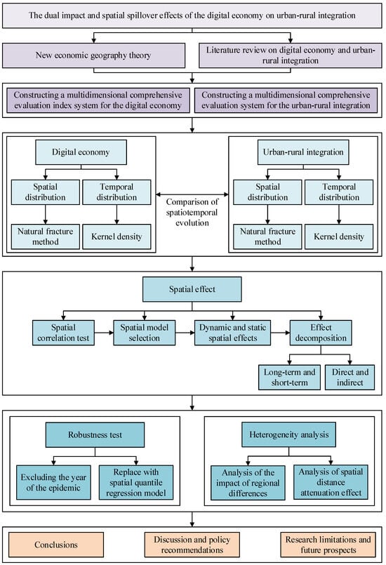
Figure 1.
Theoretical framework and technical roadmap.
3. Method, Model, and Data Source
3.1. Model Selection
3.1.1. Theoretical Basis and Logic
To explore the spatial impact and spillover effects of the DE on URI in various provinces of China, we adopted a spatial econometric model. The model selection is based on several considerations, as outlined below.
Firstly, the applicability of the spatial panel model: Select spatial panel Durbin model (SPDM), spatial panel lag model (SPLM), and spatial panel error model (SPEM) to capture spatial dependence and lag.
Secondly, the introduction of a dynamic model: Considering the time delay effect of URI, a dynamic spatial panel model is introduced to deeply analyze the long-term and short-term impacts of the DE on URI.
Thirdly, model selection process: The dynamic SPDM model is determined to be optimal through non-spatial panel model regression, the Hausman test, the F-test, the BP test, and the spatial correlation test.
3.1.2. Scientific Data Processing and Empirical Analysis
- (1)
- Data source and preprocessing
The data mainly come from the China Statistical Yearbook, China Rural Statistical Yearbook, China High tech Industry Statistical Yearbook, and provincial statistical yearbooks, covering the period from 2000 to 2021. We strictly follow the data cleaning and organization process, eliminate missing and outlier values, and use interpolation to reasonably supplement some missing data to ensure data quality.
The descriptive statistical results of the main variables involved in this article are shown in Table 1. After comparison, it can be seen that there is no significant difference in the mean and standard deviation of each variable, which is suitable for further analysis.

Table 1.
Descriptive statistical results of variables.
- (2)
- Quantitative evaluation and testing
Based on the constructed indicator system, we conducted a quantitative evaluation of the DE and URI and eliminated the issue of multicollinearity between indicators through variance inflation factor (VIF) testing, ensuring the rationality of the model set.
3.2. Classic Spatial Econometric Model
3.2.1. Spatial Autocorrelation
In existing studies, spatial effects are examined by looking at the relationship between neighboring regions. This paper aims to determine if DE and URI share similar spatial characteristics by using spatial autocorrelation indicators for verification. Commonly used indicators are the Moran index and Geary’s c ratio. However, Geary’s c ratio often produces unstable test results because it tends to deviate from the normal distribution. Therefore, the Moran index is the preferred choice in most literature. The Moran index can test whether all regions are related in terms of geographical location, and its formula is as follows:
Here, is the number of regions (31 in this paper); and are the values of the and region sum; ; , and it is the variance of ; is the 0–1 space weight matrix, when region and are near, , and when region and are not near, . At the same time, according to the Formula (1), the sum of each matrix row is set to 1 for normalization.
After standardization, the Moran index is calculated, and its value range is (−1,1).
In addition, the local Moran index can also be tested to verify the degree of correlation between the local region and its neighboring region, which is defined as:
3.2.2. Spatial Panel Econometric Model
The spatial panel econometric models consist of the SPDM, SPLM, and SPEM. A dynamic spatial panel model incorporates a time lag term for the dependent variable or a time and space lag term for the explained variable.
- (1)
- Expressions for three models
The expression of SPLM is as follows:
where is the dependent variable, is the dimensional exogenous independent variable matrix, is the spatial lag coefficient of the explained variable, reflecting the influence degree of the neighboring region’s on the URI of the region, is the spatial weight matrix, is the spatial lag explained variable, is used to explain the influence of the independent variable on the dependent variable , and is the random error term.
The expression of the SPEM is as follows:
The definitions of , , and are the same as the above model; is the spatial error correlation coefficient, reflecting the influence degree of the adjacent region’s on this region’s .
The SPDM is derived from the residual autocorrelation time series model, and its expression is as follows:
Here, is the spatial lag independent variable, and other variable definitions follow the SPLM.
The SPEM is no longer estimated using the OLS regression method because the obtained estimation results may be biased or invalid. The static spatial panel model is estimated using the maximum likelihood (ML), instrumental variable, or generalized least squares estimation. For the estimation of dynamic SPDM, there are three commonly used methods: first, the ML estimation method with bias correction or the quasi maximum likelihood (QML) estimation method; second, the instrumental variable estimation method or the generalized moment estimation method; and third, the Markov chain Monte Carlo (MCMC) method. In this paper, the static SPDM is estimated using the ML approach, and the dynamic SPDM is estimated using the QML technique.
- (2)
- Maximum likelihood estimation method
The logarithmic likelihood function of the spatial panel model is:
where is a constant, is the number of time cycles, , is the Kronecker product, and the second term in the formula represents the Jacobian term obtained from the transition of . By maximizing the likelihood function determinant, the corresponding parameters of the model can be found. If obeyed , then the likelihood function of the model is:
Finally, according to the correlation between variables, the ML function values of the corresponding model parameters can be obtained.
3.3. Spatial Quantile Regression Model
Koenker and Bassett Jr [] extended OLS and proposed a quantile regression method by fitting explanatory variables with explained variables at different loci, that is, quantile regression, and further combined quantile regression with panel data. Using the conditional quantiles of explained variables, a regression model can be obtained under different quantiles, less affected by extreme values than OLS regression. According to quantile regression, the unknown parameter can be estimated by minimizing the weighted average of the residual absolute value.
Taking the SPLM as an example, its general expression is:
where ; ; is the explanatory variable vector, is the spatial weight matrix, is the vector of the coefficient to be estimated, and is the random error term. If , then Equation (11) can be converted to:
Further, the quantile constraint is applied to Equation (11):
The spatial lag quantile regression model can be obtained:
The of Equation (12) can be regarded as an endogenous variable. Chernozhukov and Hansen [] proposed using instrumental variables to solve the endogenous problem, assuming that the instrumental variable is , then
Let , adopt and as the instrumental variable, where is the identity array and is the element in . To perform ordinary quantile regression of under the conditions of :
where , is the indicative function, is the function of , and we limit the function to satisfy . Then, the objective Equation (15) can be obtained by the following functions:
The process of parameter estimation is as follows: first, given parameter , ordinary quantile regression is carried out on Equation (16) to obtain
Secondly, minimize and obtain a consistent estimator of , where: is a positive definite matrix.
Finally, Equation (17) is a weighted quantile regression, which is obtained.
3.4. Spatial Attenuation Boundary Measure Model
According to the first law of geography, the spatial dependence between regions decreases with increasing distance. To determine the spatial attenuation boundary of the DE on URI, this paper assumes that the geographical distance interval between two provinces is [, ], denoted as as the progressive distance from to . On the basis of Equations (1) and (2), the following spatial weight matrix sequence with the function of distance progression is constructed:
where .
3.5. TOPSIS Entropy Weight Method
The entropy weighting method is an objective weighting method that uses the differences between information and weight indicators. This can better reflect the utility value of indicator information entropy. Therefore, the indicator weights obtained are more accurate and reliable than the subjective weighting method. TOPSIS is a method used for multi-objective decision-making. It can fully utilize the information of raw indicator data and rank the evaluation objects by calculating the distance between the evaluation object and the optimal and worst solutions. The results can accurately reflect the differences between various evaluation schemes. This article uses the entropy weight method to determine the weights of evaluation indicators for the quality of DE development in various regions, thereby reducing the impact of subjective weighting and improving the objectivity of evaluation. It then uses TOPSIS to evaluate the quality of DE development in various provinces of China. The basic steps of the TOPSIS entropy weight method are as follows:
- ➀
- Entropy weight method to calculate the weight of each indicator
The first step is to calculate the proportion of each indicator in each sample, :
Among them, represents the year, represents the -th province, represents the -th indicator, and represents the -th indicator of the -th province in the th year.
The second step is to calculate the information entropy of each indicator:
Among them, , .
The third step is to determine the weight of each indicator:
Among them, the smaller the entropy value of the indicator, the greater its weight , and the greater its impact on the level of DE in the evaluation results.
- ➁
- TOPSIS evaluation model
The first step is to construct a weighted decision matrix :
The standardized matrix , where represents the weight vector constructed by the entropy weight method and represents the standard value of the -th indicator weighted and normalized for the -th province in the -th year.
The second step is to use the TOPSIS method to determine the positive ideal solution and negative ideal solution :
The third step is to calculate the Euclidean distance, which is the distance between the evaluation index and the positive ideal solution, and the distance between the evaluation index and the negative ideal solution:
The fourth step is to calculate the relative proximity :
Among them, and the larger , the closer it is to the maximum value, indicating a higher level of DE.
3.6. Indicator Selection and Data Source
3.6.1. Digital Economy
To comprehensively assess the development level of the DE, this study draws on relevant domestic and international research, as well as DE indices published by global organizations, selecting evaluation indicators that align with the current state of China’s DE development. Based on prior literature [,,,], the study measures DE development using three primary indicators, validates the selection through a VIF test, and applies the TOPSIS entropy method for calculation (see Table 2).
Table 2.
Index construction of DE.
3.6.2. Urban–Rural Integration
To evaluate the level of URI development, this study references relevant research and policy documents from both domestic and international sources. Drawing on prior literature [,,], the study employs four primary indicators to assess URI, verifies the selection through a VIF test, and utilizes the mean square error method for calculation []. The details are provided in Table 3.
Table 3.
Index construction of URI.
3.6.3. Control Variables
In this paper, industry aggregation (IA) [], government intervention (GI) [], industrial structure (IS) [], technical market level (TML) [], and the extent of openness to the outside world (EO) [] are selected as the control variables (see Table 4).
Table 4.
Control variable definition table.
3.6.4. Difference from Existing Indices
The index systems for the DE and URI developed in this study represent significant advancements in both comprehensiveness and scientific rigor compared to existing indices. Existing indices often focus on a specific aspect of the DE or URI, such as digital infrastructure construction, the degree of economic integration, etc., and fail to fully reflect the complexity and diversity of these two fields. To overcome this limitation, this article extensively studied a large number of existing academic literature and gained a deep understanding of the latest concepts and definitions of the DE and URI in the academic community. On this basis, this article combines various existing indicators related to the DE and URI, and after careful screening and comprehensive consideration, finally summarizes the indicator system of this article.
This indicator system not only covers multiple aspects of the DE, including the construction of digital infrastructure, the deepening of digital industries, and the breadth of industrial digital transformation, but also comprehensively considers multiple dimensions such as the economy, society, space, and environment of URI, so as to more comprehensively reflect the actual situation of DE and URI. During the construction of this indicator system, this study placed a strong emphasis on enhancing scientific rigor by ensuring the rationality of indicator selection and data quality through rigorous data preprocessing and VIF testing.
3.6.5. The Significance of Reassessment
Reevaluating the development level of DE and URI not only helps to better understand the relationship between the two but also provides a scientific basis for policy making. Through the indicator system constructed in this study, it can be clearly seen that the DE has different impacts on URI in different regions, providing targeted policy recommendations for achieving more balanced urban–rural development.
4. Results
4.1. Analysis of Distribution Characteristics
4.1.1. Digital Economy
- (1)
- Spatial distribution angle
This paper plots the changes in the DE of various provinces in 2000, 2007, 2014, and 2021 by Arcgis10.8 and divides the DE of China into four levels using the natural break classification method, as shown in Figure 2.
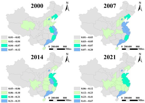
Figure 2.
Comparison of the spatial distribution of DE in different years in China.
From Figure 2, the following three analysis results are obtained.
Firstly, the spatiotemporal changes are obvious at the overall level. China’s DE has been developing steadily, and both the lower and upper limits are gradually increasing over time.
Secondly, the disparity among higher-level regions is gradually widening. Throughout each period, Guangdong and Beijing consistently ranked as the leading regions in DE development, while Shanghai, Jiangsu, Zhejiang, and other provinces have progressively formed a second tier. This trend may be attributed to the recent relocation of DE-related manufacturing industries from these provinces to other regions.
Lastly, a strong trend of agglomeration is evident. The number of provinces in the top tier of DE development is gradually declining, while those in the second and third tiers exhibit a noticeable clustering pattern. This phenomenon may result from the significant spillover effects of regions with an advanced DE, which radiate influence and drive development in surrounding areas with less-developed DEs.
- (2)
- Temporal distribution angle
The distribution, polarization phenomena, and dynamic development trends of China’s DE are analyzed in this research using the kernel density estimation method, as shown in Figure 3. In the figure, the vertical coordinate is the kernel density value measured by the Gaussian kernel function method. The horizontal coordinate represents the DE and the side axis is the time axis.
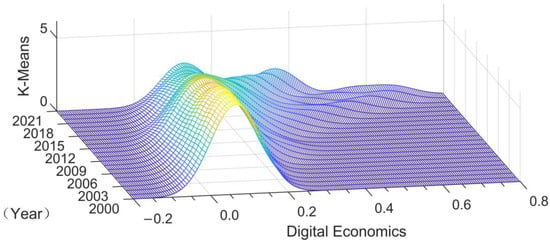
Figure 3.
3D kernel density estimation chart of China’s DE development level.
The following four analysis results are obtained from Figure 3.
Firstly, the central position of the kernel density function shifted to the right over the sample period, reflecting the overall improvement in China’s DE. Secondly, the height of the main peak of the kernel density function significantly decreased after 2015, reaching its lowest point in 2018. This indicates a reduction in disparities within China’s DE. Additionally, the fluctuations in the peak’s amplitude and direction during the study years suggest that China’s DE has been progressing in a non-linear, zigzag pattern rather than following a steady upward trend. Thirdly, in terms of distribution, the kernel density curve for DE from 2000 to 2021 exhibits a right-skewed pattern. Lastly, the presence of multiple peaks in the kernel density function during the sample period highlights a multi-polar differentiation in China’s DE development.
4.1.2. Urban–Rural Integration
- (1)
- Spatial distribution angle
This paper uses Arcgis10.8 to plot the changes in URI in each province in 2000, 2007, 2014, and 2021 and divides the URI into four levels using the natural break classification method, as shown in Figure 4.
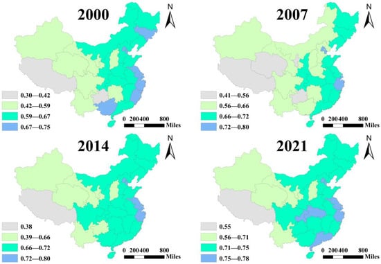
Figure 4.
Comparison of the spatial distribution of URI in different years in China.
Based on Figure 4, the spatiotemporal changes are obvious at the overall level. With the passage of time, the URI in China has significantly improved, and the number of provinces with a higher level has increased significantly.
Additionally, the agglomeration characteristics of URI are prominent, displaying a notable degree of spatial correlation marked by diversity. In the eastern regions, URI demonstrates a strong clustering trend, with these areas typically ranking in the third to fourth quartile. Conversely, in the western regions, particularly Qinghai, Tibet, and their neighboring provinces, URI exhibits weaker clustering characteristics.
Lastly, the spatial distribution of URI varies significantly across regions, with central cities serving as strong drivers of radiative influence. Specifically, Beijing and Zhejiang emerge as focal centers, with URI levels gradually declining outward from these hubs. This paper attributes this spatial pattern to a combination of geographical location and economic and social factors.
- (2)
- Temporal distribution angle
The distribution, polarization phenomena, and dynamic development trends of China’s URI are analyzed using the kernel density estimation method, as shown in Figure 5. In the figure, the vertical coordinate is the kernel density value measured by the Gaussian kernel function method, the horizontal coordinate represents the URI, and the side axis is the time axis.
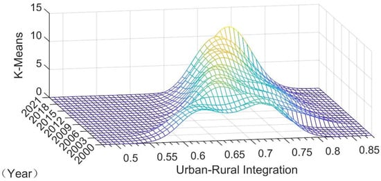
Figure 5.
3D kernel density estimation map of China’s URI.
From Figure 5, the following analysis results can be obtained.
Firstly, the center of fluctuation in the kernel density function shifts to the right, indicating a general upward trend in URI over time. Secondly, the morphology of the distribution shows that the main peak becomes higher and narrower, reflecting an increasing concentration of URI levels across regions and a decreasing degree of dispersion. Thirdly, the leftward tail of the kernel density curve is prominent, signifying that provinces with low URI levels are more scattered, highlighting significant disparities in URI among China’s 31 provinces. Finally, the kernel density distribution curve consistently exhibits a single-peak form from 2003 to 2021, indicating the persistent challenge of achieving multiple equilibria in the long-term development of China’s URI.
4.2. Spatial Effect
4.2.1. The Spatial Durbin Model
- (1)
- Variable description statistics
The descriptive statistical results of the main variables are shown in Table 5.
Table 5.
Descriptive statistical results of each variable.
As presented in Table 5, the mean value of the URI variable is 0.665, indicating that the 31 provinces in China generally demonstrate relatively strong levels of URI. The range of the URI variable is 0.502, with a standard deviation of 0.077, reflecting overall stability across the country, with only a few years or regions displaying notable variations. In contrast, the mean value of the DE variable is 0.084, suggesting that the DE in most provinces remains at a relatively low level. With a range of 0.658 and a standard deviation of 0.09, the data show that, while the national average for the DE is low, a few provinces have achieved significantly higher levels of development.
- (2)
- Spatial correlation test
A spatial weight matrix is created using geographical distance to determine if the spatial econometrics model can be used to analyze the DE and URI. The global Moran index is also calculated by converting the sectional spatial weight matrix into the spatial panel weight matrix, as shown in Table 6.
Table 6.
Global Moran index of each variable.
Table 6 reveals that the Moran index of the variable URI is 0.252 and the p-value is 0.000. This shows that the URI of 31 provinces is positively correlated with each other. The Moran index of DE is 0.305 with a p-value of 0.000, indicating that the DE of 31 provinces is positively correlated. The Moran index of each control variable is significant.
- (3)
- Choice of spatial model
The Moran Index reveals that China’s URI and DE display significant positive spatial effects, underscoring the necessity of constructing a spatial panel model. To begin, a regression analysis is performed using a non-spatial panel model. Next, the Hausman test, F-test, and BP test are applied to identify the most appropriate model—whether the mixed regression model, fixed-effects model, or random-effects model. Detailed results are presented in Table 7.
Table 7.
Results of non-spatial panel model.
The F-tests reject the null hypothesis, leading to the selection of a fixed-effects model. Similarly, the BP test also rejects the null hypothesis in favor of a fixed-effects model over mixed regression. The Hausman test further rejects the null hypothesis, confirming the appropriateness of a fixed-effects model over a random-effects model. Together, these tests validate the selection of a fixed-effects model.
Within the fixed-effects framework, the maximum likelihood function (Lagl) value for the time fixed-effects model is notably small, and the R2 value for the double fixed-effects model is also relatively low. Following the principle that higher R2 and Lagl values indicate a better fit, the spatial fixed effects model is deemed more suitable. Additionally, the LM and RLM tests confirm the validity of both the SPLM and the SPEM. Therefore, further consideration is given to the feasibility of the SPDM under spatial fixed effects.
As can be seen from Table 8, both the LR test and the Wald test reject the null hypothesis of and , so it is better to choose the SPDM.
Table 8.
The LR test and Wald test results of the model.
To sum up, the SPDM under the spatial fixed effect is selected in this paper.
- (4)
- Model estimation
Based on the above series of tests, the explained variable is also affected by the time factor; therefore, the time lag term is considered to establish the dynamic SPDM:
where is the regression coefficient of the time lag term and is the correlation coefficient of the spatial lag term. Details are presented in Table 9.
Table 9.
Regression results of static and dynamic SPDM.
From Table 9, in the static spatial fixed-effects model, the spatial lag term of the DE is significantly positively correlated with the URI of the explained variable. In the dynamic spatial fixed-effects model, the time lag term of URI exhibits a significant positive correlation, while the spatial lag term also demonstrates a significant positive relationship. The coefficient of 0.6539 indicates a strong model fit. However, in the dynamic spatial fixed-effects model, the spatial lag term of the DE shows a significant negative correlation with the URI of the explained variable, which deviates from expected norms and warrants further investigation. Table 10 shows the results of the DE’s direct, indirect, and total effects on URI from the perspectives of static and dynamic spatial fixed-effects models.
Table 10.
Effect decomposition of static and dynamic spatial fixed-effect models.
From Table 10, the static model only reports long-term effects.
The spillover effect of the DE on URI is positive, with the total effect also being positive, while the direct effect of DE on URI is negative. This indicates that, in the static spatial fixed-effects model, the impact of DE on URI is predominantly driven by indirect effects. Additionally, the total effects of the control variables on URI are significant and are largely determined by their spillover effects.
The dynamic model reports both short-term and long-term effects. The total short-term effect of the DE is estimated at −4.20, while the long-term effect is 0.47, both of which are statistically significant. According to the results in Table 10, the dynamic impact of DE on URI remains negative in the short term, primarily driven by immediate effects. However, the long-term impact is positive, aligning with observed trends over time. Furthermore, the signs of the coefficients in the dynamic model are largely consistent with those in the static model, indicating minimal deviation in the direction of impact and the spillover effects of each explanatory variable on URI.
4.2.2. Robustness Test
- (1)
- Replace the spatial model
This paper selects the spatial lag term of tax burden level [] as the instrumental variable for spatial quantile regression.
Table 11 shows that the DE has a significant evolutionary effect on the level of URI. Firstly, the spatial quantile regression model shows that the DE has a significant negative impact at different quantile points, consistent with the results of the spatial Durbin model. This reaffirms the earlier conclusion that while the long-term impact of China’s DE on URI is positive, its current short-term effects remain predominantly negative. Additionally, at the five quantiles of 0.1, 0.3, 0.5, 0.7, and 0.9, the DE coefficients are −0.217, −0.259, −0.225, −0.175, and −0.133, respectively. The absolute values of these coefficients initially increase and then decrease, suggesting that the spatial impact of the DE on URI is influenced by the regional tax burden. In regions with either high or low tax burden levels, the DE’s promotion effect on URI is relatively limited.
Table 11.
Results of spatial quantile regression.
- (2)
- The data of the pandemic year were excluded
Considering the possible uncertain impact of the epidemic on regional development after 2020, this paper excludes the data of the abnormal years after the pandemic, namely 2020 and 2021.
By comparing the results of Table 9 and Table 12, it can be found that the regression results of the SPDM before and after excluding the data of the pandemic year are identical. It shows that although the pandemic greatly impacted China’s economy, the trend of the DE’s impact on URI has not changed fundamentally. Similarly, it also indicates the robustness of this research’s conclusions, which are not affected by specific time periods.
Table 12.
Results of the SPDM after the elimination of the pandemic year.
4.2.3. Heterogeneity Analysis
- (1)
- Regional heterogeneity analysis
There are obvious differences in the geographical environment, resource endowment, talent introduction policies, and other aspects in different regions. This could lead to different impacts on the development of URI due to the six major factors: the development levels of the DE, IA, GI, IS, TML, and EO. As a result, this study divides China into three regions (excluding the Taiwan region), as seen in Figure 6.
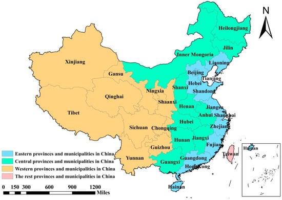
Figure 6.
Map of regions in China.
The heterogeneity of influencing factors in different regions on URI is further explored; for details, see Table 13.
Table 13.
Results of the SPDM by region.
From Table 13, the static fixed-effects model indicates that while the DE in the eastern region has a significant positive impact on URI, its regression coefficient is much smaller in absolute value compared to that of the DE in the western region. This discrepancy results in an overall negative impact of the DE on URI. Additionally, the spatial lag term of the DE in the central and western regions shows a significant positive correlation with the dependent variable at the 1% level, suggesting a notable spatial spillover effect. In these regions, the development of the DE in one area can drive URI processes in neighboring areas.
In the dynamic fixed-effects model, the regression coefficients for the eastern, central, and western regions are all significant, with R-squared values of 0.85, 0.87, and 0.82, respectively, indicating strong model fit. The DE in the eastern region exhibits a significant positive impact on URI, consistent with observed trends. In contrast, the DE in the central region has a significant negative impact on URI, potentially due to uneven regional economic development, disparities in urban–rural economic foundations, and the relatively lagging overall economic progress in the central region. As a result, the DE in the central region has constrained the development of URI.
- (2)
- Measurement of spatial spillover boundary
According to New Economic Geography, the economic influence of various economic activities or regions tends to decrease with the increase in spatial distance; thus, there is distance attenuation. To investigate the attenuation possibility boundary of the DE’s spatial effects on the URI, the spatial weight matrix of the possible attenuation boundary is constructed, and the SPDM regression analysis is conducted.
Since the shortest geographical distance between the two provinces is 96.073 km, this paper starts from 90 km and takes every 50 km as the progressive distance for continuous regression (i.e., every 50 km for regression); for details, see Table 14.
Table 14.
Spatial decay process of DE affecting the URI.
From Table 14 and Figure 7, it can be seen that under both static and dynamic spatial fixed-effects models, the impact of the DE on the URI of surrounding areas shows a decreasing trend, accompanied by fluctuations. The increase in distance causes the spatial overflow coefficient to fluctuate and increase due to the influence of outliers. When the distance exceeds 540 km, the spatial spillover effect decreases sharply. Therefore, the spatial spillover effect of the DE on adjacent-region URI is significant within one to two provinces or 540 km, and then weakens with increasing distance.
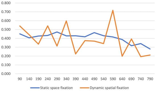
Figure 7.
Attenuation boundary of spatial spillover effect.
5. Conclusions
This study employs advanced econometric methods, such as SPDM, to deeply analyze the complex relationship and spatial spillover effects between China’s DE and URI. Based on extensive empirical data and theoretical frameworks, the following core conclusions are drawn:
Firstly, regarding the spatiotemporal evolution characteristics of the DE and URI, the research reveals distinct regional differences. The eastern region leads in DE and URI development due to its advanced economic foundation, robust policy support, and abundant talent and technological resources. However, in recent years, this region has experienced a downward trend, likely driven by resource and environmental constraints and efforts to optimize industrial structures. In contrast, the western region faces challenges from a weaker economic foundation and lower levels of DE and URI, resulting in insufficient growth momentum. These findings reflect the uneven development of China’s regional economy and underscore both the potential and challenges of advancing the DE across different regions.
Secondly, with respect to the dual impact of the DE, the research findings indicate that the DE’s influence on URI exhibits significant dual characteristics. In the short term, uneven technological diffusion and lagging infrastructure development may exacerbate the urban–rural divide, resulting in suppressive effects on URI. However, over the long term, increased technological penetration and optimized resource allocation drive URI, fostering coordinated development between urban and rural areas. This finding not only confirms the hypothesis of short-term suppression and long-term promotion but also provides theoretical insights into the complex mechanisms underlying the DE’s impact.
Thirdly, acknowledging the importance of spatial spillover effects, the use of spatial panel econometric models and spatial attenuation boundary measurement models confirms that the DE exerts significant spillover effects on URI. These effects are evident not only in the direct influence on local URI but also in the indirect impact on surrounding areas through spatial transmission mechanisms. In the short term, these spatial spillover effects may be negative, reflecting transitional challenges; however, they gradually evolve into positive impacts over time. This finding underscores the diffusion and spillover characteristics of the DE across spatial dimensions, offering a critical foundation for designing policies that foster regional coordinated development.
Fourthly, the research highlights significant regional differences in the DE’s promotion effect on URI. In the eastern region, the DE has consistently and significantly promoted URI due to its strong economic foundation, optimized industrial structure, and robust technological innovation capabilities. In the central region, despite certain economic and industrial advantages, the promotion effect of the DE remains constrained by resource and environmental limitations, as well as challenges related to industrial transformation and upgrading. Conversely, the western region exhibits a relatively weak promotion effect from the DE, primarily due to its underdeveloped economic foundation, insufficient talent resources, and limited technological innovation capacity. These findings highlight the disparities in regional economic development across China and offer empirical support for designing differentiated and region-specific development policies.
6. Discussion and Policy Recommendations
6.1. Comparative Analysis with Existing Research in the Academic Community
This section aims to systematically compare and evaluate the findings of this study within the broad context of the existing academic literature.
6.1.1. Spatiotemporal Evolution of Digital Economy
Firstly, the DE across China’s regions exhibits a distinct pattern of “Eastern High, Western Low, with Declines in Both the East and West”. This disparity can be attributed to the relatively weaker factor endowment and resource allocation in the central and western regions, resulting in lower DE levels, consistent with previous studies []. Additionally, the spatial distribution of the DE closely resembles that of digital inclusive finance []. This article posits that this pattern is shaped not only by the level of regional economic development but also by factors such as policy orientation, talent mobility, and technological innovation. These elements collectively influence the spatiotemporal evolution of the DE, leading to the observed imbalance
Secondly, the spatiotemporal distribution of the high-level DE and digital finance is slightly different. In the digital financial inclusion index [], Shanghai has consistently held the top ranking. However, in the same period, since 2014, Shanghai’s DE level has fallen behind that of Beijing and Guangdong. This may be due to the recent transfer of most manufacturing industries from Shanghai to Jiangsu, Zhejiang, and Anhui, leading to a contraction of DE-related physical manufacturing industries and ultimately causing a relative decline in Shanghai’s DE level. In addition, as an international financial center, Shanghai’s DE development relies more on the service and financial industries rather than the manufacturing industry, which also explains the relationship between its DE level and the transfer of the manufacturing industry.
6.1.2. Spatiotemporal Evolution of the Urban–Rural Integration
URI across China’s regions exhibits a distinct pattern of “Eastern High, Western Low, with Declines in Both the East and West”. Existing research highlights long-standing regional inequalities in China [], particularly between the developed eastern regions and the underdeveloped central and western areas []. This disparity is clearly reflected in URI levels []. Contributing factors in the western region include a fragile ecological environment, outdated transportation infrastructure, unfavorable geographical conditions, talent outflows, financial deficits, and a lack of technological advancement. These challenges collectively undermine sustainable development and hinder URI growth. The interplay of these factors significantly influences the spatiotemporal evolution of URI, resulting in the current imbalanced state.
Moreover, changes in URI in different parts of China are mostly influenced by the local urban–rural wealth division. According to the existing literature, the overall inequality in China is mainly affected by the disparity between urban and rural income []. Meanwhile, China’s income gap has long been dominated by urban–rural disparities []. In addition, China’s urbanization level [] and financial level [] have had a positive effect on the urban–rural income gap, leading to further widening of the gap. However, it is worth noting that with the government’s implementation of poverty alleviation policies and rural revitalization strategies in rural areas, the pace of URI has accelerated in recent years but regional differences are still significant.
6.1.3. The Impact of Digital Economy on Urban–Rural Integration
Firstly, the DE has a dual impact on URI. Man et al. [] considered the digital industry to be the main driver in enhancing the coupling and coordination of the Chinese DE and URI. Meng [] noted that the widespread adoption of DE infrastructure has increased agricultural production efficiency. However, due to the existence of the digital division [], urban and rural households continue to differ in the acquisition, processing, and creation of digital resources, resulting in new inequality caused by a widening income gap. This dual impact is not only related to the penetration rate of digital technology but also to various factors such as the level of regional economic development, talent reserves, and policy environment. When digital technology penetration is poor, urban and rural disparities will grow, and as the penetration of digital technology increases, the use of digital technology in rural and urban areas will gradually converge, which will benefit the poor and reduce the income gap between urban and rural []. This article argues that this convergence process is not smooth sailing and requires joint efforts from the government, enterprises, and various sectors of society to promote the popularization and application of digital technology.
Additionally, the dual impact of the DE on URI has a spatial spillover effect. The empirical results indicate that the DE has a significant regional spillover effect on URI, which is also supported by the related literature. For example, Cheng and Zheng [] found that the positive influence of the DE on the coordination of city and countryside has significant positive spatial spillover. Hao and Ji [] argue that platform economies based on emerging technologies have spatial spillover effects. The expansion effect of the DE on the income disparity between urban and rural areas has significant spatial spillover []. The existence of such spatial spillover effects means that the development of the DE in a region will not only affect the URI process in the local area but also have significant impacts on surrounding areas. Therefore, when formulating relevant policies, it is necessary to fully consider this spatial spillover effect in order to achieve coordinated development between regions.
6.2. Multidimensional Interpretation of Results
This study depicts, in detail, the uneven distribution pattern of the DE among provinces in China from the perspective of spatiotemporal evolution. The eastern provinces have shown a clear first-mover advantage, while the western region is in a rapid catching-up stage. This distribution feature is highly consistent with the evolution path of URI, further verifying the role of the DE as the core driving force of URI. It is worth noting that the differences between static and dynamic models reveal the complexity and dynamic characteristics of the impact of the DE. In the short term, the DE may have a certain constraining effect on URI due to resource competition. However, the significant positive effect of its spatial lag term indicates that the DE has a strong spatial spillover effect, which effectively promotes coordinated development between regions. In the long run, the positive impact of the DE on URI is more prominent, highlighting its potential as a long-term economic growth engine.
6.3. Critical Reflection on Current Policies
Although the current policy framework has made some progress in promoting the integration of the DE and URI, it still faces challenges such as insufficient regional adaptability and a lack of deep integration mechanisms. Specifically, the policy formulation process did not fully consider regional differences, resulting in an uneven implementation of policies. Similarly, the policy focus is mostly on infrastructure construction and technological innovation, neglecting the key link of effective transformation and application of DE achievements in urban and rural areas. To address these challenges, this study recommends adopting differentiated policy strategies tailored to regional characteristics. Efforts should focus on enhancing the integration mechanisms between the DE and URI. This includes accelerating the translation of DE advancements into practical URI outcomes through policy incentives, fostering collaboration among industry, academia, and research institutions, and promoting the application of digital technologies. Such measures aim to achieve balanced and sustainable urban–rural development.
6.4. Response and Discussion of Research Hypotheses
Based on the literature review and preliminary research results, this study proposed four core hypotheses regarding the relationship between the DE and URI in Section 2.3. The following subsections present a detailed discussion and verification of these hypotheses.
6.4.1. Spatiotemporal Changes and Co-Evolution Trends
Hypothesis 1 proposes that the spatiotemporal changes in the DE and URI follow a similar evolutionary trajectory, driven by a common external environment and internal mechanisms, exhibiting an evolutionary trend from low to high, from local to global, and from single to multiple, with a regular spatial distribution. Through data analysis and model validation, this study reveals a positive correlation between the development of the DE and URI, with both exhibiting similar spatial trends. Over the long term, both demonstrate gradual improvement and diffusion, supporting Hypothesis 1 regarding their co-evolutionary trajectory. However, this co-evolution is not entirely synchronous, as it involves time lags and spatial disparities. These findings provide a foundation for further exploration of the complex relationship between the DE and URI.
6.4.2. Dual Characteristics of Short-Term Inhibition and Long-Term Promotion
Hypothesis 2 states that the DE has a dual characteristic of short-term suppression and long-term promotion on URI. In the short term, the uneven popularization of technology and lagging infrastructure may exacerbate the urban–rural gap. In the long run, technological penetration will promote resource optimization and advance the process of URI. Through empirical analysis, we found that the DE has indeed had a certain inhibitory effect on URI in the short term, mainly attributed to the initial stage of technology application, where there are significant differences in technology acquisition capabilities and infrastructure construction between urban and rural areas. However, in our long-term observations, with the deepening penetration of technology and the optimization of resource allocation, the promotional effect of DE on URI gradually emerges, verifying the dual characteristics of hypothesis 2.
6.4.3. Spatial Spillover Effect
Hypothesis 3 suggests that the DE has significant spatial spillover effects on URI, influencing surrounding areas through channels such as technology diffusion and knowledge dissemination, promoting interdependence and coordinated development of economic activities. In this study, we conducted an in-depth analysis of the spatial spillover effects of the DE using spatial panel econometric models and spatial attenuation boundary measurement models. The results indicate that the DE does have significant spatial spillover effects, and the development of the DE in a region can not only promote URI in the local area but also have a positive impact on URI in surrounding areas. The existence of such spatial spillover effects further confirms the correctness of hypothesis 3 and provides an important basis for us to formulate regional coordinated development strategies.
6.4.4. Regional Heterogeneity
Hypothesis 4 emphasizes that regional heterogeneity plays an important role in the relationship between the DE and URI. Due to differences in economy, industry, and resources in different regions, the promotion effect of the DE on URI varies significantly. In this study, we found significant regional differences in the impact of the DE on URI through a heterogeneity analysis of the eastern, central, and western regions of China. Especially in the western region, due to the relatively weak economic foundation, the promotional effect of the DE on URI is relatively limited. This discovery validates hypothesis 4 regarding regional heterogeneity and suggests that when formulating relevant policies, we should fully consider regional differences and implement differentiated regional development strategies.
In summary, this study has verified the rationality and effectiveness of the proposed hypothesis through an in-depth analysis of the relationship between the DE and URI. These findings not only enrich the theoretical research in the field of DE and URI but also provide a scientific basis and useful references for formulating relevant policies and practices. Future research can further explore the dynamic relationship and impact mechanism between the DE and URI, providing more theoretical support and practical guidance for promoting the development of URI.
6.5. Policy Recommendations
To promote the potential of the DE and accelerate the URI process, this article recommends the following policies:
Firstly, the government and policymakers should strengthen the construction of digital economic infrastructure to support URI. During the URI process, special emphasis should be placed on the balanced distribution and sustainable development of digital economic infrastructure. For central and western regions, as well as rural areas, it is essential to increase investment, enhance the accessibility and application of digital technologies, and ensure equitable access to digital resources between urban and rural areas. Simultaneously, priority should be given to the environmentally sustainable construction and maintenance of infrastructure to promote the development of a green DE, thereby providing long-term support for URI.
Secondly, policymakers should establish a sustainable urban–rural-integrated DE policy environment. They should develop and refine a policy and regulatory framework that supports the integrated development of urban and rural areas, ensuring long-term stability and effectiveness. The deep integration of the DE with URI should be facilitated through targeted policy guidance and support to drive coordinated economic, social, and cultural development across urban and rural areas. Furthermore, policy oversight and evaluation mechanisms should be enhanced to ensure the effectiveness and sustainability of these initiatives, providing robust institutional support for URI.
Thirdly, when formulating DE-related policies, it is essential to consider spatial spillover effects and regional heterogeneity to foster balanced development between urban and rural areas. Establishing a regional DE cooperation mechanism that integrates urban and rural areas can facilitate information sharing, technology exchange, and talent mobility, driving coordinated regional development. Additionally, optimizing resource allocation and protecting the ecological environment across urban and rural areas will further support sustainable economic, social, and environmental development.
Fourthly, the cultivation and recruitment of DE talent for URI should be strengthened. Thus, the talent development system in the DE sector should be deepened, with a particular focus on nurturing individuals with innovative capabilities and practical experience. This can be achieved when talent cultivation and recruitment in rural and peri-urban areas to bridge gaps in expertise are prioritized. Also, special funds and training bases to enhance the skills and qualifications of DE professionals should be established, ensuring sustained talent support for URI.
Fifthly, differentiated policies for an urban–rural-integrated DE should be implemented. DE policies to address the specific needs of different regions and urban–rural contexts should be tailored. For the eastern region and urban centers, policymakers should encourage the exploration of new models and formats for integrating the DE with the real economy. This will enhance quality and efficiency. For the central and western regions, as well as rural areas, policy support to accelerate the growth of DE industries should be increased. Moreover, resource conservation and environmental protection should be emphasized, promoting balanced development between urban and rural areas.
7. Research Limitations and Future Prospects
7.1. Research Limitations
Although this study uses cutting-edge econometric methods such as dynamic spatial panel models to deeply analyze the complex relationship and spatial spillover effects between China’s DE and URI, there are still some limitations, mainly reflected in the following aspects:
Firstly, data availability and timeliness: The data used in this study primarily originate from publicly accessible statistical sources and the literature. However, due to limitations in data availability and timeliness, they may not fully capture the most recent developments in the DE and URI. Future research should aim to explore and incorporate more comprehensive and up-to-date data sources to enhance the accuracy and relevance of the analysis.
Secondly, regional division and heterogeneity analysis: This study adopted a broad classification of regions into eastern, central, and western zones but did not delve deeply into the heterogeneity characteristics of more granular regional divisions. Future research could employ finer regional classification methods to better uncover the development disparities and impact mechanisms of the DE across different areas.
Thirdly, model setting and variable selection: Although this study endeavored to maintain scientific rigor in model design and variable selection, certain subjective choices and limitations may remain. Future research could consider introducing additional relevant variables and refining model frameworks to provide a more comprehensive understanding of the relationship between the DE and URI.
Fourthly, evaluation of policy implementation effectiveness: This study primarily focuses on the impact mechanisms and spatial spillover effects of the DE on URI, with limited emphasis on assessing the effectiveness of policy implementation. Future research could integrate case studies of specific policies to analyze their impacts on the DE and URI in greater depth, offering targeted recommendations for policy-making.
7.2. Future Prospects
Based on the limitations of the above research, this study proposes the following future prospects:
Firstly, enhance data mining and utilization: Future research should explore and integrate richer data sources, such as social media data, enterprise survey data, and other emerging datasets, to improve the accuracy and timeliness of analyses. This approach will better capture the latest trends in the DE and URI, providing a more comprehensive perspective.
Secondly, refine regional division and heterogeneity analysis: Future studies can adopt more nuanced regional division methods, incorporating factors such as city size, economic development levels, or industrial characteristics. This refinement would allow for a more precise understanding of the developmental disparities and impact mechanisms of the DE across different regions.
Thirdly, optimize model settings and variable selection: Future research can introduce additional relevant variables, such as technological advancement, industrial structure transformation, and resource allocation, to enhance model robustness. By doing so, researchers can gain a more comprehensive understanding of the relationship between the DE and URI and delve deeper into the underlying factors influencing this relationship.
Fourthly, strengthen the evaluation of policy implementation effectiveness: Future studies can incorporate specific policy case analyses to evaluate the impacts of policies on the DE and URI. This would include assessing the effectiveness of policy implementation and providing targeted recommendations for future policy design. Additionally, establishing a systematic policy effectiveness evaluation framework could offer a scientific basis for optimizing and adjusting policies to better support DE and URI development.
Author Contributions
Conceptualization, J.B. and D.T.; methodology, J.B.; software, J.B.; validation, J.B., D.T. and Y.F.; formal analysis, J.B.; investigation, J.B.; resources, J.B.; data curation, J.B.; writing—original draft preparation, J.B.; writing—review and editing, D.T. and Y.F.; visualization, D.T. and Y.F.; supervision, D.T.; project administration, D.T. All authors have read and agreed to the published version of the manuscript.
Funding
This research received no external funding.
Institutional Review Board Statement
Not applicable.
Informed Consent Statement
Not applicable.
Data Availability Statement
The raw data supporting the conclusions of this article will be made available by the authors upon request.
Conflicts of Interest
The authors declare no conflicts of interest.
References
- Ye, X.; Christiansen, F. China’s urban-rural integration policies. J. Curr. Chin. Aff. 2009, 38, 117–143. [Google Scholar] [CrossRef]
- Xi, J. Report at the 19th National Congress of the Communist Party of China. In Proceedings of the 19th National Congress of the Communist Party of China, Beijing, China, 18–24 October 2017. (In Chinese). [Google Scholar]
- Meng-Xu, M.-X. A Comparative Study of the English Translation of the Reports to the 19th and the 20th National Congress of the Communist Party of China from the Perspective of Corpus-based Critical Translation Studies, SHS Web of Conferences. EDP Sci. 2023, 168, 02013. [Google Scholar] [CrossRef]
- Miller, H.J. Tobler’s first law and spatial analysis. Ann. Assoc. Am. Geogr. 2004, 94, 284–289. [Google Scholar] [CrossRef]
- Liu, G.; Liu, B. How digital technology improves the high-quality development of enterprises and capital markets: A liquidity perspective. Financ. Res. Lett. 2023, 53, 103683. [Google Scholar] [CrossRef]
- Pouri, M.J.; Hilty, L.M. The digital sharing economy: A confluence of technical and social sharing. Environ. Innov. Soc. Transit. 2021, 38, 127–139. [Google Scholar] [CrossRef]
- Tapscott, D. The Digital Economy: Promise and Peril in the Age of Networked Intelligence; McGraw-Hill: New York, NY, USA, 1996. [Google Scholar]
- Shapiro, C.; Varian, H.R. Information Rules: A Strategic Guide to the Network Economy; Harvard Business Press: Boston, MA, USA, 1999. [Google Scholar]
- Moulton, B.R. GDP and the Digital Economy: Keeping Up with the Changes; Bureau of Economic Analysis, US Department of Commerce: Suitland, MD, USA, 1999; pp. 34–48. [Google Scholar] [CrossRef]
- Kling, R.; Lamb, R. IT and organizational change in digital economies: A socio-technical approach. ACM SIGCAS Comput. Soc. 1999, 29, 17–25. [Google Scholar] [CrossRef]
- Carlsson, B. The Digital Economy: What is new and what is not? Struct. Change Econ. Dyn. 2004, 15, 245–264. [Google Scholar] [CrossRef]
- Purnomo, A.; Susanti, T.; Rosyidah, E.; Firdausi, N.; Idhom, M. Digital economy research: Thirty-five years insights of retrospective review. Procedia Comput. Sci. 2022, 197, 68–75. [Google Scholar] [CrossRef]
- Ma, Q.; Tariq, M.; Mahmood, H.; Khan, Z. The nexus between digital economy and carbon dioxide emissions in China: The moderating role of investments in research and development. Technol. Soc. 2022, 68, 101910. [Google Scholar] [CrossRef]
- Liu, J.; Yang, Y.; Zhang, S. Research on the measurement and driving factors of China’s digital economy. Shanghai J. Econ. 2020, 6, 81–96. [Google Scholar] [CrossRef]
- Heping, G.; Fuxiang, W. Digital Economy Enables High-Quality Economic Development: Theoretical Mechanisms and Empirical Evidence. Front. Econ. China 2022, 17, 643. [Google Scholar] [CrossRef]
- Guo, C.; Song, Q.; Yu, M.-M.; Zhang, J. A digital economy development index based on an improved hierarchical data envelopment analysis approach. Eur. J. Oper. Res. 2024, 316, 1146–1157. [Google Scholar] [CrossRef]
- Li, Z.; Liu, Y. Research on the spatial distribution pattern and influencing factors of digital economy development in China. IEEE Access 2021, 9, 63094–63106. [Google Scholar] [CrossRef]
- Tranos, E.; Reggiani, A.; Nijkamp, P. Accessibility of cities in the digital economy. Cities 2013, 30, 59–67. [Google Scholar] [CrossRef]
- Duc, D.T.V.; Dat, T.T.; Linh, D.H.; Phong, B.X. Measuring the digital economy in Vietnam. Telecommun. Policy 2024, 48, 102683. [Google Scholar] [CrossRef]
- Hosan, S.; Karmaker, S.C.; Rahman, M.M.; Chapman, A.J.; Saha, B.B. Dynamic links among the demographic dividend, digitalization, energy intensity and sustainable economic growth: Empirical evidence from emerging economies. J. Clean. Prod. 2022, 330, 129858. [Google Scholar] [CrossRef]
- Tao, C.; Peng, Y. Spatial effects of technological innovation intensity on the upgrading of industrial structure under economic agglomeration. Ind. Econ. Res. 2017, 3, 91–103. [Google Scholar] [CrossRef]
- Lordan, G.; Neumark, D. People versus machines: The impact of minimum wages on automatable jobs. Labour Econ. 2018, 52, 40–53. [Google Scholar] [CrossRef]
- Yang, Q.; Ma, H.; Wang, Y.; Lin, L. Research on the influence mechanism of the digital economy on regional sustainable development. Procedia Comput. Sci. 2022, 202, 178–183. [Google Scholar] [CrossRef]
- Ranis, G.; Fei, J.C. A theory of economic development. Am. Econ. Rev. 1961, 51, 533–565. Available online: https://www.jstor.org/stable/1812785 (accessed on 1 November 2023).
- Preston, D.A. Rural-urban and inter-settlement interaction: Theory and analytical structure. Area 1975, 7, 171–174. [Google Scholar]
- Baker, J. Survival and accumulation strategies at the rural-urban interface in north-west Tanzania. Environ. Urban. 1995, 7, 117–132. [Google Scholar] [CrossRef] [PubMed]
- Torreggiani, D.; Dall’Ara, E.; Tassinari, P. The urban nature of agriculture: Bidirectional trends between city and countryside. Cities 2012, 29, 412–416. [Google Scholar] [CrossRef]
- Liu, Y.; Li, Y. Revitalize the world’s countryside. Nature 2017, 548, 275–277. [Google Scholar] [CrossRef]
- Long, H.; Tu, S.; Ge, D.; Li, T.; Liu, Y. The allocation and management of critical resources in rural China under restructuring: Problems and prospects. J. Rural Stud. 2016, 47, 392–412. [Google Scholar] [CrossRef]
- He, J.; Jin, X.B.; Liang, X.Y.; Zhao, Q.L.; Han, B.; Xiao, Y.; Wu, X.H.; Hu, J.; Zhou, Y.K. Research of rural system development potential in Huaihai Economic Zone: A case study of Northern Jiangsu province under the background of urban-rural integration. J. Nat. Resour. 2020, 35, 1940–1957. [Google Scholar] [CrossRef]
- Liu, Y.; Long, H.; Li, Y. Human geography research based on the new thinking of global rural-urban relationship. Acta Geogr. Sin. 2021, 76, 2869–2884. [Google Scholar] [CrossRef]
- Xiu, C.-L.; Xu, D.-M.; Zhu, X.-L. Evaluation of urban-rural integration course in northeast China. Sci. Geogr. Sin. 2004, 24, 325–331. (In Chinese) [Google Scholar]
- Shi, J.; Duan, K.F.; Wu, G.; Li, J.; Xu, K. Efficiency of urban-rural integration development in the Yangtze River Delta under the background of carbon emission constraint. Econ. Geogr. 2021, 41, 57–67. [Google Scholar] [CrossRef]
- Xuemei, L.; Yamin, L.; Lingxiang, H. The Spatio-Temporal Evolution and Influencing Factors Underlying the Development of Urban-Rural Integration in the Counties of Hebei Province, China. J. Resour. Ecol. 2024, 15, 317–328. [Google Scholar] [CrossRef]
- Zhang, C.; Fan, Y.; Fang, C. Orderly and synergistic development of urban-rural integration based on evolutionary game model: A case study in the Jiangxi Province, China. Land Use Policy 2024, 146, 107331. [Google Scholar] [CrossRef]
- Zeng, Q.; Chen, X. Identification of urban-rural integration types in China–an unsupervised machine learning approach. China Agric. Econ. Rev. 2023, 15, 400–415. [Google Scholar] [CrossRef]
- Ovaska, U.; Vihinen, H.; Oostindie, H.; Farinós, J.; Hrabar, M.; Kilis, E.; Kobal, J.; Tisenkopfs, T.; Vulto, H. Network governance arrangements and rural-urban synergy. Sustainability 2021, 13, 2952. [Google Scholar] [CrossRef]
- Rickardsson, J. The urban–rural divide in radical right populist support: The role of resident’s characteristics, urbanization trends and public service supply. Ann. Reg. Sci. 2021, 67, 211–242. [Google Scholar] [CrossRef]
- Boudet, F.; MacDonald, G.K.; Robinson, B.E.; Samberg, L.H. Rural-urban connectivity and agricultural land management across the Global South. Glob. Environ. Chang. 2020, 60, 101982. [Google Scholar] [CrossRef]
- Seale, E. Coping strategies of urban and rural welfare organisations and the regulation of the poor. New Political Econ. 2013, 18, 141–170. [Google Scholar] [CrossRef]
- Baier, N.; Pieper, J.; Schweikart, J.; Busse, R.; Vogt, V. Capturing modelled and perceived spatial access to ambulatory health care services in rural and urban areas in Germany. Soc. Sci. Med. 2020, 265, 113328. [Google Scholar] [CrossRef]
- Yang, Y.; Bao, W.; Wang, Y.; Liu, Y. Measurement of urban-rural integration level and its spatial differentiation in China in the new century. Habitat Int. 2021, 117, 102420. [Google Scholar] [CrossRef]
- Yang, Y.; Liu, Y.; Li, Y.; Li, J. Measure of urban-rural transformation in Beijing-Tianjin-Hebei region in the new millennium: Population-land-industry perspective. Land Use Policy 2018, 79, 595–608. [Google Scholar] [CrossRef]
- Ma, L.; Liu, S.; Fang, F.; Che, X.; Chen, M. Evaluation of urban-rural difference and integration based on quality of life. Sustain. Cities Soc. 2020, 54, 101877. [Google Scholar] [CrossRef]
- Zhang, H.; He, R.; Li, G.; Wang, J. Spatiotemporal evolution of coupling coordination degree of urban-rural integration system in metropolitan area and its influencing factors: Taking the capital region as an example. Econ. Geogr. 2020, 40, 56–67. [Google Scholar] [CrossRef]
- Chen, Z.; Lu, M. From segmentation to integration: The political economy of urban–rural economic growth and social harmony. Econ. Res. J. 2008, 1, 21–32. (In Chinese) [Google Scholar]
- Zhou, M.; Guo, F.; Sun, Y.; Ren, J.; Zhang, X. Promotion or inhibition? Exploring the influence of the digital economy on urban-rural integration: A case study of yellow River basin. Sustain. Futures 2024, 8, 100293. [Google Scholar] [CrossRef]
- Du, B.; Wang, Y.; He, J.; Li, W.; Chen, X. Spatio-temporal characteristics and obstacle factors of the urban-rural integration of China’s shrinking cities in the context of sustainable development. Sustainability 2021, 13, 4203. [Google Scholar] [CrossRef]
- Zhao, H.; Zheng, X.; Yang, L. Does digital inclusive finance narrow the urban-rural income gap through primary distribution and redistribution? Sustainability 2022, 14, 2120. [Google Scholar] [CrossRef]
- Liu, X.; Han, Q. The influence of internet usage of rural residents on income and its mechanism—Based on China family panel studies (CFPS) data. J. Agrotech. Econ. 2018, 9, 123–134. [Google Scholar] [CrossRef]
- Zhang, B.; Wu, W. Digital Inclusive Finance, Entrepreneurship and Income Distribution: An Empirical Research from the Perspective of Urban-rural Differences in China. Chin. Rev. Financ. Stud. 2021, 13, 31–44. (In Chinese) [Google Scholar]
- Xun, Z.; Guanghua, W.; Jiajia, Z.; Zongyue, H. Digital economy, financial inclusion and inclusive growth. China Econ. 2020, 15, 92–105. [Google Scholar] [CrossRef]
- Xiufeng, B.T.; Yating, W.; Xianming, K. Internet trade development and income distribution gap. Ind. Technol. Econ. 2020, 39, 107–115. (In Chinese) [Google Scholar]
- He, D.; Han, X.; Li, Y. Factors affecting consumers’ purchase intention in electronic commerce of fresh agro-products. J. Northwest AF Univ. 2014, 14, 85–91. [Google Scholar] [CrossRef]
- Salemink, K.; Strijker, D.; Bosworth, G. Rural development in the digital age: A systematic literature review on unequal ICT availability, adoption, and use in rural areas. J. Rural Stud. 2017, 54, 360–371. [Google Scholar] [CrossRef]
- Philip, L.J.; Townsend, L.; Roberts, E.; Beel, D. The rural digital economy. Taylor Fr. 2015, 131, 143–147. [Google Scholar] [CrossRef]
- Jun, L. An empirical study on the urban-rural digital divide that continues to widen the urban-rural income gap. Stat. Decis 2017, 33, 119–121. [Google Scholar] [CrossRef]
- Yaping, H.; Canning, X. The impact of the Internet on the urban-rural income gap: A test based on Chinese facts. Econ. Econ. 2019, 36, 25–32. [Google Scholar]
- Hou, X.; Zhang, D.; Fu, L.; Zeng, F.; Wang, Q. Spatio-temporal evolution and influencing factors of coupling coordination degree between urban–rural integration and digital economy. Sustainability 2023, 15, 9718. [Google Scholar] [CrossRef]
- Fong, M.W. Digital divide between urban and rural regions in China. Electron. J. Inf. Syst. Dev. Ctries. 2009, 36, 1–12. [Google Scholar] [CrossRef]
- Wang, Y.; Peng, Q.; Jin, C.; Ren, J.; Fu, Y.; Yue, X. Whether the digital economy will successfully encourage the integration of urban and rural development: A case study in China. Chin. J. Popul. Resour. Environ. 2023, 21, 13–25. [Google Scholar] [CrossRef]
- Huang, J.; Jin, H.; Ding, X.; Zhang, A. A study on the spatial correlation effects of digital economy development in China from a non-linear perspective. Systems 2023, 11, 63. [Google Scholar] [CrossRef]
- Ye, Q.; Cao, X. Research on the Heterogeneity of Digital Economy Driving Regional Integration Development: Comparative Analysis Based on Three Major Urban Agglomerations. Int. J. Educ. Humanit. 2022, 4, 187–191. [Google Scholar] [CrossRef]
- Koenker, R.; Bassett, G., Jr. Regression quantiles. Econom. J. Econom. Soc. 1978, 46, 33–50. [Google Scholar] [CrossRef]
- Chernozhukov, V.; Hansen, C. Instrumental quantile regression inference for structural and treatment effect models. J. Econom. 2006, 132, 491–525. [Google Scholar] [CrossRef]
- Chinoracky, R.; Corejova, T. How to evaluate the digital economy scale and potential? Entrep. Sustain. Issues 2021, 8, 536. [Google Scholar] [CrossRef] [PubMed]
- Brynjolfsson, E.; Collis, A. How should we measure the digital economy. Harv. Bus. Rev. 2019, 97, 140–148. [Google Scholar]
- Strassner, E.H.; Nicholson, J.R. Measuring the digital economy in the United States. Stat. J. IAOS 2020, 36, 647–655. [Google Scholar] [CrossRef]
- Xu, Y.; Li, T. Measuring digital economy in China. Natl. Account. Rev. 2022, 4, 251–272. [Google Scholar] [CrossRef]
- De, Z.; Jia, Q.; Wen, Z. Review of urban-rural integration evaluation: Connotation identification, theoretical analysis, and system reconstruction. J. Nat. Resour. 2021, 36, 2634–2651. [Google Scholar] [CrossRef]
- Shan, B.; Zhang, Q.; Ren, Q.; Yu, X.; Chen, Y. Spatial heterogeneity of urban–rural integration and its influencing factors in Shandong province of China. Sci. Rep. 2022, 12, 14317. [Google Scholar] [CrossRef]
- He, Y.; Zhou, G.; Tang, C.; Fan, S.; Guo, X. The spatial organization pattern of urban-rural integration in urban agglomerations in China: An agglomeration-diffusion analysis of the population and firms. Habitat Int. 2019, 87, 54–65. [Google Scholar] [CrossRef]
- Zhao, W.; Jiang, C. Analysis of the Spatial and Temporal Characteristics and Dynamic Effects of Urban-Rural Integration Development in the Yangtze River Delta Region. Land 2022, 11, 1054. [Google Scholar] [CrossRef]
- Li, H.; Tian, H.; Rabbi, M.A. The impact of informatization on the urban-rural income gap: An empirical investigation of China. Inf. Dev. 2023, 39, 02666669231210839. [Google Scholar] [CrossRef]
- Shi, X.; Jiang, Z. Opening to the Outside World and Income Gap between Urban and Rural Areas Based on Panel Data of 30 Provinces and Cities. Front. Bus. Econ. Manag. 2022, 5, 161–166. [Google Scholar] [CrossRef]
- Wang, X.; Piesse, J. Inequality and the urban–rural divide in China: Effects of regressive taxation. China World Econ. 2010, 18, 36–55. [Google Scholar] [CrossRef]
- Wang, W.; Yang, X.; Cao, J.; Bu, W.; Adebayo, T.S.; Dilanchiev, A.; Ren, S. Energy internet, digital economy, and green economic growth: Evidence from China. Innov. Green Dev. 2022, 1, 100011. [Google Scholar] [CrossRef]
- Zhang, G.; Chen, Y.; Wang, G.; Zhou, C. Spatial-temporal evolution and influencing factors of digital financial inclusion: County-level evidence from China. Chin. Geogr. Sci. 2023, 33, 221–232. [Google Scholar] [CrossRef]
- Yu, C.; Jia, N.; Li, W.; Wu, R. Digital inclusive finance and rural consumption structure–evidence from Peking University digital inclusive financial index and China household finance survey. China Agric. Econ. Rev. 2022, 14, 165–183. [Google Scholar] [CrossRef]
- Fujita, M.; Hu, D. Regional disparity in China 1985–1994: The effects of globalization and economic liberalization. Ann. Reg. Sci. 2001, 35, 3–37. [Google Scholar] [CrossRef]
- Li, Y.; Wei, Y.D. The spatial-temporal hierarchy of regional inequality of China. Appl. Geogr. 2010, 30, 303–316. [Google Scholar] [CrossRef]
- Wang, Y.; Liu, Y.; Li, Y.; Li, T. The spatio-temporal patterns of urban–rural development transformation in China since 1990. Habitat Int. 2016, 53, 178–187. [Google Scholar] [CrossRef]
- Sicular, T.; Ximing, Y.; Gustafsson, B.; Shi, L. The urban–rural income gap and inequality in China. Rev. Income Wealth 2007, 53, 93–126. [Google Scholar] [CrossRef]
- Zhao, X.; Hao, G.; Wang, Y.; Xie, X.; Wen, X.; Cao, L.; Ye, S.; Lin, M. Analysis of the Urban-Rural Income Gap in China. J. Sociol. Ethnol. 2022, 4, 46–56. [Google Scholar]
- Ye, Z.; Qian, L.; Na, Z. Financial development, urbanization, and urban-rural income disparity: Evidence based on Chinese provincial data. Mod. Econ. 2018, 9, 31–60. [Google Scholar] [CrossRef]
- Tao, J. Empirical Study on the Relationship between Financial Development and Urban and Rural Residents’ Income Gap in Guangdong Province. Am. J. Ind. Bus. Manag. 2020, 10, 219–231. [Google Scholar] [CrossRef][Green Version]
- Man, J.; Liu, J.; Cui, B.; Sun, Y.; Sriboonchitta, S. Coupling and coordination between digital economy and Urban–Rural Integration in China. Sustainability 2023, 15, 7299. [Google Scholar] [CrossRef]
- Meng, X. Analysis of the dual impact of digital economy on urban-rural income gap. Front. Bus. Econ. Manag. 2023, 7, 34–36. [Google Scholar] [CrossRef]
- Furuholt, B.; Kristiansen, S. A rural-urban digital divide? Regional aspects of Internet use in Tanzania. Electron. J. Inf. Syst. Dev. Ctries. 2007, 31, 1–15. [Google Scholar] [CrossRef]
- Sun, X.; Kuang, X. Will advances in digital technology reduce the rural-urban income gap? Econ. Res. -Ekon. Istraživanja 2023, 36, 2194954. [Google Scholar] [CrossRef]
- Cheng, Y.; Zheng, D. Does the Digital Economy Promote Coordinated Urban–Rural Development? Evidence from China. Sustainability 2023, 15, 5460. [Google Scholar] [CrossRef]
- Hao, N.; Ji, M. Development of platform economy and urban–rural income gap: Theoretical deductions and empirical analyses. Sustainability 2023, 15, 7684. [Google Scholar] [CrossRef]
- Deng, X.; Guo, M.; Liu, Y. Digital economy development and the urban-rural income gap: Evidence from Chinese cities. PLoS ONE 2023, 18, e0280225. [Google Scholar] [CrossRef]
Disclaimer/Publisher’s Note: The statements, opinions and data contained in all publications are solely those of the individual author(s) and contributor(s) and not of MDPI and/or the editor(s). MDPI and/or the editor(s) disclaim responsibility for any injury to people or property resulting from any ideas, methods, instructions or products referred to in the content. |
© 2025 by the authors. Licensee MDPI, Basel, Switzerland. This article is an open access article distributed under the terms and conditions of the Creative Commons Attribution (CC BY) license (https://creativecommons.org/licenses/by/4.0/).