Article

Decoding China’s Transport Decarbonization Pathways: An Interpretable Spatio-Temporal Neural Network Approach with Scenario-Driven Policy Implications

1
College of Transportation, Shandong University of Science and Technology, Qingdao 266590, China
2
International Cooperation Center of National Development and Reform Commission, Beijing 100038, China
*
Author to whom correspondence should be addressed.
Sustainability 2025, 17(15), 7102; https://doi.org/10.3390/su17157102
Submission received: 27 June 2025 / Revised: 23 July 2025 / Accepted: 4 August 2025 / Published: 5 August 2025

Abstract

The transportation sector, as a major source of carbon emissions, plays a crucial role in the realization of dual carbon goals worldwide. In this study, an improved least absolute shrinkage and selection operator (LASSO) is used to identify six key factors affecting transportation carbon emissions (TCEs) in China. Aiming at the spatio-temporal characteristics of transportation carbon emissions, a CNN-BiLSTM neural network model is constructed for the first time for prediction, and an improved whale optimization algorithm (EWOA) is introduced for hyperparameter optimization, finding that the prediction model combining spatio-temporal characteristics has a more significant prediction accuracy, and scenario forecasting was carried out using the prediction model. Research indicates that over the past three decades, TCEs have demonstrated a rapid growth trend. Under the baseline, green, low-carbon, and high-carbon scenarios, peak carbon emissions are expected in 2035, 2031, 2030, and 2040. The adoption of a low-carbon scenario represents the most advantageous pathway for the sustainable progression of China’s transportation sector. Consequently, it is imperative for China to accelerate the formulation and implementation of low-carbon policies, promote the application of clean energy and facilitate the green transformation of the transportation sector. These efforts will contribute to the early realization of dual-carbon goals with a positive impact on global sustainable development.

1. Introduction

In 2020, China set dual-carbon targe [1]. Confronted with this ambition, carbon emissions have emerged as a central concern, requiring rigorous attention to diverse segments of Chinese society. The Chinese government has positioned the “energy conservation and emissions reduction” strategy as a fundamental pillar of sustainable long-term development. As a vital component supporting socioeconomic development [2], the proliferation of the national economy and urbanization has rendered the transport sector a major source of global carbon emissions [3]. According to calculations presented in this study, between 1990 and 2019, TCEs surged from 104 to 916 million tons, demonstrating a rapid growth trajectory. By 2019, TCEs had exceeded one-tenth of the total carbon emissions in China [4]; decarbonization of transportation is imperative. Transport decarbonization refers to reducing carbon emissions in the transportation sector through technological innovation, energy transition, policy guidance, and model optimization, with the ultimate goal of achieving carbon neutrality, given the important role of the transportation sector in achieving our overall carbon peaking goals [5]. Accurate prediction of TCEs is the basis for formulating scientific emission reduction policies. This study constructs a precise prediction model to provide quantitative evidence and decision support for low-carbon transportation development.
Currently, scholarly inquiry into carbon emissions primarily focuses on two pivotal dimensions: initially, the elucidation of the principal determinants that shape transportation-related carbon emissions, and, subsequently, the advancement of more precise predictive frameworks for estimating TCEs. Identifying the principal determinants can assist policymakers not only in formulating targeted policies and measures to reduce emissions but also in enhancing the precision of emission prediction models by using these factors as input feature variables. Developing a more precise model for predicting TCEs can help policymakers in forecasting future emissions trends, serving as a pivotal foundation for the development and refinement of policies, as well as for enhancing policy effectiveness. Consequently, undertaking in-depth research into the principal determinants, along with the development of highly accurate predictive models, holds substantial strategic significance for fostering green transportation growth and realizing the objectives of low-carbon urban environments.
Within the sphere of determining the principal determinants, prominent research methodologies include the stochastic impacts by regression on population, affluence and technology model (STIRPAT), logarithmic mean Divisia index method (LMDI), generalized Divisia index model (GDIM), and grey relational analysis method, among others. For instance, Zhao et al. [6] employed the STIRPAT model to project the anticipated peak in TCE infrastructure-building activities in Liaoning Province. Sun et al. [7] conducted an in depth investigation into the impact of seven factors on TCE efficiency within the Yangtze River Economic Belt by constructing a STIRPAT model. Zhang et al. [8] used LMDI to study carbon emission drivers and put forward suggestions for TCE reduction. Luo et al. [9] employed the LMDI model to meticulously analyze the temporal evolution of TCEs in the Guangdong–Hong Kong–Macao Greater Bay Area, as well as the driving factors. Zhang et al. [10] employed the Grey Relational Analysis technique to examine the determinants of carbon emissions in Shandong Province, finding that passenger turnover and freight volume were the most significant indicators. Nevertheless, these models presuppose linear correlations among variables and therefore may encounter difficulties in accounting for multifaceted factors that influence TCEs. The LASSO regression model is very effective in managing high-dimensional data, selecting important influencing factors, and reducing problems related to multicollinearity and overfitting. However, considering the heterogeneity and complexity that may exist in actual data, and to further improve the overall performance of the model, the present study further adopts the improved LASSO model to conduct a more in-depth analysis of the factors affecting TCEs and to model TCEs more accurately.
In the construction of algorithms for TCE prediction models, traditional models often employ methods such as establishing Kaya identity and STIRPAT model to intuitively predict TCEs. For instance, Lin et al. [11] addressed the persistently high levels of TCEs by employing the Kaya model to explore the core factors influencing carbon emissions. They also conducted a quantitative assessment of the carbon emissions and mitigation potential under various predefined scenarios. Guo et al. [12] utilized a combined approach of the STIRPAT model to predict the trajectory of TCEs in Henan Province from 2020 to 2060, resulting in a timetable for TCE predictions. Li et al. [13] employed GM(1,1) and BP models to forecast TCEs in Beijing before 2030, which serves as a crucial basis for designing and implementing Beijing’s carbon reduction strategy and determining its future trajectory. Janhuaton et al. [14] used an ANN model to project TCEs in Thailand under different scenarios, emphasizing the effectiveness of policy scenarios in reducing carbon emissions. Liu et al. [15] trained seven machine learning algorithms, including random forests and XGBoost, and concluded that interprovincial differences were the most influential factor, with the XGBoost algorithm showing the most significant predictive effect. Liu et al. [16] used Grey Relational Analysis (GRA) to filter influencing factors, and then utilized the BiLSTM model to learn the temporal sequence characteristics of these factors, so as to predict the incidence of new energy vehicles in China’s automotive fleet, and to calculate the carbon reduction amount. Huang et al. [17] used a model combining LSTM and SVR to predict TCEs, and, based on China’s actual situation, they put forward such suggestions as strengthening the management of carbon assets of enterprises and deploying carbon emission reduction techniques. Ekaterina et al. [18], targeting New York City’s carbon neutrality goals, analyzed and predicted carbon emissions by employing four distinct machine learning algorithms, and selected the most effective algorithm to predict New York City’s carbon emissions from 2021 to 2050. Iftikhar et al. [19] have introduced a method that combines regression and time series analysis to forecast an upward trend in carbon emissions in Pakistan. In light of these findings, it is imperative for the government to enact measures to mitigate carbon emissions. Compared with traditional methods, neural network models have stronger data fitting capabilities and the ability to handle nonlinear relationships, effectively capturing the complex characteristics and dynamic changes of TCEs, thus providing more precise and flexible prediction results.
Research on TCE prediction models has mostly constructed single neural network prediction models [20], either time series or spatial feature prediction models, with fewer studies combining time series prediction with spatial feature prediction models. However, TCEs not only exhibit obvious temporal characteristics but also has significant spatial correlation characteristics across different regions [21,22,23]. The monolithic predictive models for forecasting TCEs suffer from the limitations of neglecting spatio-temporal interactions and inadequate generalization capabilities, thus struggling to comprehensively integrate multifaceted influences. In contrast, the spatio-temporal integrated model is more capable of accurately capturing the spatio-temporal features of TCE data, thereby enhancing predictive accuracy and adaptability. Therefore, this paper proposes a spatio-temporal coupled prediction framework based on CNN-BiLSTM for resolving the spatio-temporal evolution law of TCEs. Convolution and pooling operations, unique to convolutional neural networks, are introduced to construct feature extractors with local connectivity characteristics, thereby effectively capturing geospatial information in the data. Building on this, we combine the bidirectional time propagation mechanism of BiLSTM to establish a dynamic recurrent unit with time-dependent resolution capabilities. Its unique memory gating system not only alleviates the gradient dispersion problem in deep network training but also achieves multi-scale temporal feature decoupling of carbon emission migration processes through joint modeling of forward and backward time series. Predicting transportation carbon emissions from a spatio-temporal perspective effectively extracts the spatio-temporal features of data, and at the same time introduces the EWOA optimization algorithm for hyper-parameter optimization of the model, aiming to achieve the best prediction effect. The model provides an interpretable prediction tool for regional carbon peak path simulation, which provides strong support for carbon emission management and policy formulation.

2. Methods

2.1. Carbon Emission Accounting Methods

In 2006, IPCC proposed two methods for accounting for carbon emissions from energy consumption: the “top-down” approach and the “bottom-up” approach. The “bottom-up” approach requires statistics on stock, transport mileage, and energy consumption per unit of distance for various modes of transportation. However, China’s existing data do not cover such information; therefore, this study adopts the “top-down” macro measurement method to calculate TCEs [24]. TCEs of each type of energy were calculated using the following equation:
C = i C i = i E i × A L H i × 10 9 × A H C i × R i × 10 3 × 44 / 12
In Equation (1), C is TCEs, i means the various types of energy necessary, including raw coal, gasoline, and kerosene, etc., E i is the physical consumption of the energy of the category i, A L H i is the average low-level heat of the energy of category i, A H C i is the carbon content per unit of calorific value of the energy of category i, and R i is the carbon emission factor of energy of category i.

2.2. LASSO Model

The LASSO model, as a refined linear regression technique, constitutes an iterative improvement in statistical regression analysis. It introduces a penalty function to compress the coefficients of variables with minor influence to zero, with these variables considered nonsignificant. This process facilitates the selection of characteristics. When dealing with high-dimensional data, the LASSO algorithm effectively reduces the risk of overfitting [25], increases the prognostic efficacy of the model, and shows good robustness and interpretability.
β ^ = arg min β k t = 1 n y t β 0 k = 1 p y t k β k 2 + λ 1 k = 1 p | β k |
In order to reduce the bias of nonzero parameter estimation, different penalty weights are assigned to different parameters in this study; smaller weight coefficients are used to penalize variables with larger initial parameter estimates and larger weight coefficients are used to penalize variables with smaller initial values, which can effectively correct the estimation bias of the model parameters. The specific expressions are as follows:
β ^ = arg min β k t = 1 n y t β 0 k = 1 p y t k β k 2 + λ 2 k = 1 p ω k | β k |
ω k = 1 | β ^ k | γ 1
where β ^ is the estimate of the regression coefficient, β ^ is the regression coefficient, λ is the non-negative regularization parameter, n denotes the total number of observations within the dataset, | β k | is the penalty term for model parameter b that shrinks the model regression coefficients toward zero, λ 1 and λ 2 are Lasso penalty weights, γ 1 is the Lasso penalty parameter, and k denotes the initial estimate of the kth model parameter [26,27].

2.3. EWOA-CNN-BiLSTM Model

2.3.1. EWOA

Whale Optimization Algorithm (WOA), as a meta-heuristic optimization algorithm inspired by nature, simulates the behavioral pattern of humpback whales’ group preying on fish by collaborating to form a bubble net, and transforms the whale’s predation strategy into a mathematical optimization process. It constructs a mathematical model by encircling the prey, bubble net attacking, and random searching the three core behaviors. The specific expressions are as follows.
(1)
Surrounding prey behavior
The whale group gradually narrows the encirclement circle by sensing the position of the current optimal individual. Each whale adjusts its position according to the direction of the optimal individual, and its moving distance is controlled by the dynamic coefficients (A and C). The mathematical model of the encirclement stage is as follows.
D = C X best X t
X ( t + 1 ) = X best A D
where t denotes the current number of iterations, X t and X t + 1 are the positions of the whales in generation t and t + 1 , and X best is the position of the optimal current solution. A is the convergence factor and C is the swing factor, denoted as follows.
A = 2 a r a
C = 2 r
where a gradually decreases from 2 to 0 as the number of iterations increases, and r is a random vector between [0, 1].
(2)
Bubble net attack
The whale rises toward the position of the optimal individual in a spiral path, while simulating the behavior of spitting out the bubble net. This process is realized through the spiral equation, which simulates the mathematical model of the spiral spitting bubble predation method.
D = X best X t
X ( t + 1 ) = D e b l cos ( 2 π l ) + X best
where D denotes the distance between the current whale and the optimal whale, b is a constant for the logarithmic spiral, and l is a random number uniformly distributed on [−1, 1].
(3)
Stochastic Search
When the population does not detect an optimal solution, some whales break away from the current enclosure and randomly select other individuals as reference targets swim away. By introducing random perturbation, the algorithm jumps out of the local extreme value region, expands the global exploration range, and enhances the search ability for the unknown solution space. The model is represented as follows.
D = C X rand X t
X t + 1 = X rand A D
where X rand denotes the position vector of a randomly selected whale in the current whale population.
Although WOA shows potential in many fields, it still faces the dual challenges of insufficient population diversity and poor convergence robustness in complex optimization tasks. To address the fluctuation of search efficiency caused by initial population randomness, this study adopts Tent chaotic mapping to reconstruct the initialization process, and ensures the uniformity of the solution space coverage through a deterministic traversal strategy, thus weakening the algorithm’s sensitivity to the initial conditions. Meanwhile, in order to overcome the premature convergence defect of the standard WOA due to linear parameter settings, a nonlinear time-varying adaptive weighting mechanism is innovatively introduced, which realizes an autonomous balance between global exploration and local exploitation capabilities by dynamically adjusting the individual search step size and information interaction strength. This has significantly enhanced the algorithm’s convergence stability and optimization accuracy.
(1)
Population initialization
The initialization process is reconstructed using Tent chaotic mapping to improve the search speed of the algorithm. The initialized population can be expressed as:
X i + 1 = X i / 0.6 0 < X i 0.6 ( 1 X i ) / ( 1 0.6 ) 0.6 < X i 1
(2)
Nonlinear time-varying inertia weights
The model control parameters are adjusted by introducing nonlinear adaptive weighting factors, which change slowly at the initial stage to maintain the global search, and drop rapidly at the later stage to improve the local development accuracy. The nonlinear time-varying inertia weights are defined as follows.
ω = 0.1 × ( 1 + cos ( ( t / M ax iter ) π ) ) 1 k t M ax iter / 2 0.1 × ( 1 cos ( ( π + ( t / M ax iter ) π ) ) ) 1 k t > M ax iter / 2
Therefore Equations (10) and (12), after introducing the new nonlinear time-varying adaptive weighting factor ω , are updated as
X ( t + 1 ) = ω D e b l cos ( 2 π l ) + X best
X ( t + 1 ) = X rand ω A D
where t is the current number of iterations, M ax iter is the maximum number of iterations, ω denotes the inertia weight, and X best is the current best whale position.

2.3.2. CNN Model

CNN exploits the properties of local connectivity and parameter sharing through convolutional and pooling layers used to extract salient features from the input data and transforms the output complex features using fully connected layers [28]. The convolution kernel is an important element in CNN, which is used to slide the input data and perform convolution operations to extract local features and resultant feature maps [29], as in Equation (5).
C j = f ( w i A i + b i )
where f is the activation function, w i is the weight, ⊙ is the convolution operation, A i is the input vector, and b i is the bias matrix.

2.3.3. BiLSTM Model

When addressing datasets with extended sequence lengths, the traditional LSTM is prone to information loss in the forward flow of the sequence. BiLSTM addresses this issue by incorporating a pair of distinct LSTM layers oriented in opposite directions. Its intrinsic architecture consists of a tandem of LSTM models arranged in a bidirectional stack, enabling the capture of contextual information from both forward and backward perspectives, which can simultaneously capture the forward and reverse long-term dependencies in the input sequence, and improve the model prediction precision and the efficacy of feature data exploitation [30].
LSTM can maintain and convey important information in long sequences by introducing gating mechanisms to control the inflow and outflow of information [31]. It is computed as follows:
f t = σ w f × [ h t 1 , x t ] + b f
i t = σ ( w i × [ h t 1 , x t ] + b i )
C ˜ t = t a n h ( w c × [ h t 1 , x t ] + b c )
O t = σ ( w o × [ h t 1 , x t ] + b o )
C t = f t C t 1 + i t C ˜ t
h t = O t tanh ( C t )
where f t , i t , and O t represent the forgetting gate, input gate, and output gate at time t, respectively. x t , h t , C ˜ t , and C t represent the input value, output value, update gate, and final cell state, respectively. σ and tanh represent the activation functions. w and b represent the weight and bias matrices, respectively [32].
The final output y t of BiLSTM is computed by calculating the forward hidden layer state h t 1 with the backward hidden layer state h t 2 , and then connecting the two hidden layer states by the corresponding weight coefficients. The specific computation process is as follows:
h t 1 = L S T M ( X t , h t 1 )
h t 2 = L S T M ( X t , h t + 1 )
y t = w h 1 × h t 1 + w h 2 × h t 2 + b y
where w h 1 is the weight matrix associated with the forward recurrent layer, w h 2 is the weight matrix pertinent to the backward recurrent layer, and b y is the bias matrix.

2.3.4. EWOA-CNN-BiLSTM Model Construction

In this study, we propose a hybrid spatio-temporal deep learning architecture for TCE data prediction, aiming to solve the modeling challenges of high-dimensional spatio-temporal sequence data. As is shown in Figure 1, the framework realizes the intelligent configuration of model parameters and joint mining of spatio-temporal features through a multi-stage collaborative optimization mechanism: firstly, the global optimization of hyper-parameters is completed based on the EWOA optimization algorithm, and the key parameters such as the number of nodes in the hidden layer, L2 regularization coefficients, and the learning rate are dynamically determined; secondly, the unique convolution and pooling operations of convolutional neural networks are introduced to construct the feature extractor with local connectivity characteristics, to effectively capture the geospatial data in the data. On this basis, we couple the bidirectional time propagation mechanism of BiLSTM to establish a dynamic recursive unit with time-dependent resolution capability, and its unique memory gating system not only alleviates the gradient dispersion problem in the training of deep networks, but also realizes the multi-scale temporal feature decoupling of the carbon emissions migration process through the joint modeling of the forward and backward time sequences. It also realizes the decoupling of multi-scale temporal features of the pollutant migration process through the joint modeling of forward and backward time series [33]. Experiments show that the architecture can significantly improve the prediction accuracy compared with the traditional methods through the synergistic optimization of the parameter space and the feature space, while guaranteeing the generalization ability of the model.

2.3.5. Evaluation Criteria

To gauge the forecasting accuracy of the model, the present research utilizes RMSE, MAE, and MAPE to analyze the prediction model, calculated as follows.
RMSE = 1 n i = 1 n ( Y i Y ^ i ) 2
MAE = 1 n i = 1 n | Y i Y ^ i |
R 2 = 1 i = 1 n Y i Y ^ ι 2 i = 1 n ( Y i Y ¯ ι ) 2
MAPE = 1 n i = 1 n Y i Y ^ i Y i
where Y i is the actual dependent variable values, Y ^ i is the predicted dependent variable value, Y ¯ is the mean value of the dependent variable, and n is the sample size.

2.4. Research Flow

To facilitate the precise assessment and future projection of TCEs, this study employs a macro-level top-down approach to meticulously calculate TCEs from 1990 to 2019. Six key influencing factors are identified for the improved LASSO regression model: GDP of the tertiary sector, population size, passenger turnover, freight, freight turnover, and transportation gasoline consumption. Subsequently, a TCE prediction model is constructed, with the aforementioned key factors as input feature parameters and the amount of TCEs as the output feature parameter, and the model is trained. To validate the prediction accuracy, the WOA-CNN-BiLSTM, Transformer, and CNN models are established for comparison. Based on the trained TCE prediction model, this study sets up four prediction scenarios to provide insights into the impact of various scenarios and policy measures on TCEs between 2020 and 2050. Drawing on the findings, this study delineates a set of strategic recommendations aimed at facilitating the green transformation of the transportation, and promoting its sustainable and high-quality development (Figure 2).

3. Results

3.1. Carbon Emissions Accounting Results

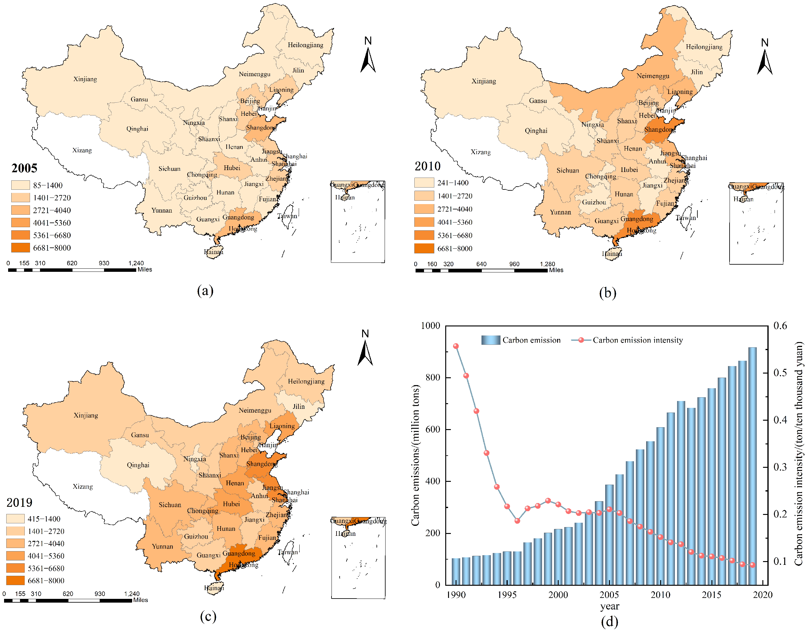
TCE is calculated (Figure 3) with Equation (1). In the time dimension, TCE shows a fluctuating upward trend, reflecting that with the economic growth and population increase, the transportation demand continues to rise, leading to an increase in carbon emissions. In terms of spatial distribution, TCE shows a pattern of high in the east and low in the west, and high in the south and low in the north, with the gap widening year by year, which indicates that there are significant differences in transportation infrastructure, types of transportation means, and energy consumption in different regions.

3.2. LASSO Regression Characterization Variable Screening Results

In the variable selection process of this study, we fully considered the multidimensional driving mechanisms of carbon emissions from transportation systems and their policy implementation requirements. Based on authoritative research frameworks and policy documents from both domestic and international sources [23,25,34,35], we systematically constructed an initial set of variables from five key dimensions: economic indicators, demographic scale, transport capacity, societal factors, and energy composition (Table 1). This selection is grounded in the theoretical foundations of the driving factors behind transportation carbon emissions while closely aligning with the actual development characteristics and policy orientations of China’s transportation sector. This ensures that the selected variables can comprehensively characterize the carbon emission features of transportation systems, laying the foundation for constructing a scientifically sound and comprehensive research framework for transportation decarbonization. Taking into account the timeliness and accessibility of data samples, the current research gathers panel data from 30 Chinese provinces from 1990 to 2019 (excluding Tibet and the Hong Kong and Macau Special Administrative Regions, as well as Taiwan). The data are sourced from “China Statistical Yearbook”. For missing data, interpolation methods are used to fill the gaps.
If these 18 key factors are input into the prediction model as parameters, it could lead to an overly complex algorithmic structure and result in overfitting. In light of this, this study utilizes the LASSO regression algorithm for feature selection, with the objective of pinpointing the critical factors that are most strongly linked to carbon emissions (Figure 4).
Using the improved LASSO regression model for feature variable selection, six variables are ultimately identified as significant: GDP of the tertiary sector (X3), population (X6), passenger turnover (X8), freight (X9), freight turnover (X11), and transportation gasoline consumption (X17). Pearson analysis is performed on the screened key factors, and the specific values and correlation results are shown in Figure 5. The correlations between TCEs and key factors are all greater than 0.95, all of which are strongly correlated, indicating that the selected variables are reasonable.

3.3. EWOA-CNN-BiLSTM Neural Network Prediction Models

3.3.1. Data Preprocessing

Before constructing EWOA-CNN-BiLSTM, the main feature variables obtained from the improved LASSO regression and carbon emissions are normalized to eliminate the influence of features with different scales. This guarantees that the model can derive proficient feature representations from the dataset, which in turn boosts the training efficacy of the model and refines its predictive performance. The formula for normalization is as follows.
X i t = X i t min ( X i ) max ( X i ) min ( X i )
where X i denotes the value of the ith influencing factor and X i t denotes the value of the ith influencing factor at the tth moment.

3.3.2. Projected Results

Before the construction of the carbon emission model, this study adopts a systematic intelligent algorithm comparative analysis framework, and selects the Sparrow Search Algorithm (SSA), Whale Optimization Algorithm (WOA), Gray Wolf Optimization Algorithm (GWO), and Marine Predator Algorithm (MPA) as the baseline references (Figure 6a). The results of the simulation experiments show that the EWOA developed in this study exhibits significant advantages in both convergence speed and global search capability, and its iterative curves show faster convergence rates and are less likely to get trapped in local optimal solutions.
The results of LASSO regression feature selection is taken as the input variable of the prediction model, and TCE is taken as the output variable of the model. The EWOA algorithm is used for global optimization to find the optimal parameters of the prediction model, and the optimal hyperparameter combinations of the prediction model are determined as follows: the number of nodes in the hidden layer of the bidirectional LSTM is 29, the initial learning rate is 0.0012, and the L2 regularization coefficient is 0.000116.
On this basis, a hybrid EWOA-CNN-BiLSTM prediction architecture integrating time-series feature extraction and dynamic parameter optimization is constructed: the input layer receives a multi-source time-series data stream with dimensions of [6 × 1 × 1], and a two-stage one-dimensional convolutional kernel (3 × 1) is used to perform local feature capture; the number of filters follows the principle of the feature pyramid to increase from 16 to 32, which is nonlinearly activated by ReLU and then activated through the sequence folding–expanding mechanism coupled with a bidirectional LSTM layer (the number of bidirectional gating units is dynamically optimized by EWOA), and its end time-step output pattern can synchronously model the long- and short-term carbon emission driving mechanisms. The architecture balances the model complexity through the adaptive regularization constraint (L2 = 0.000116), and combines with the dynamic learning rate scheduling of the Adam optimizer, which effectively improves the generalized prediction accuracy of the carbon emission time-series trajectories. The input data is shuffled, and the prediction performance of the EWOA model on the training and test sets is shown in Figure 6.
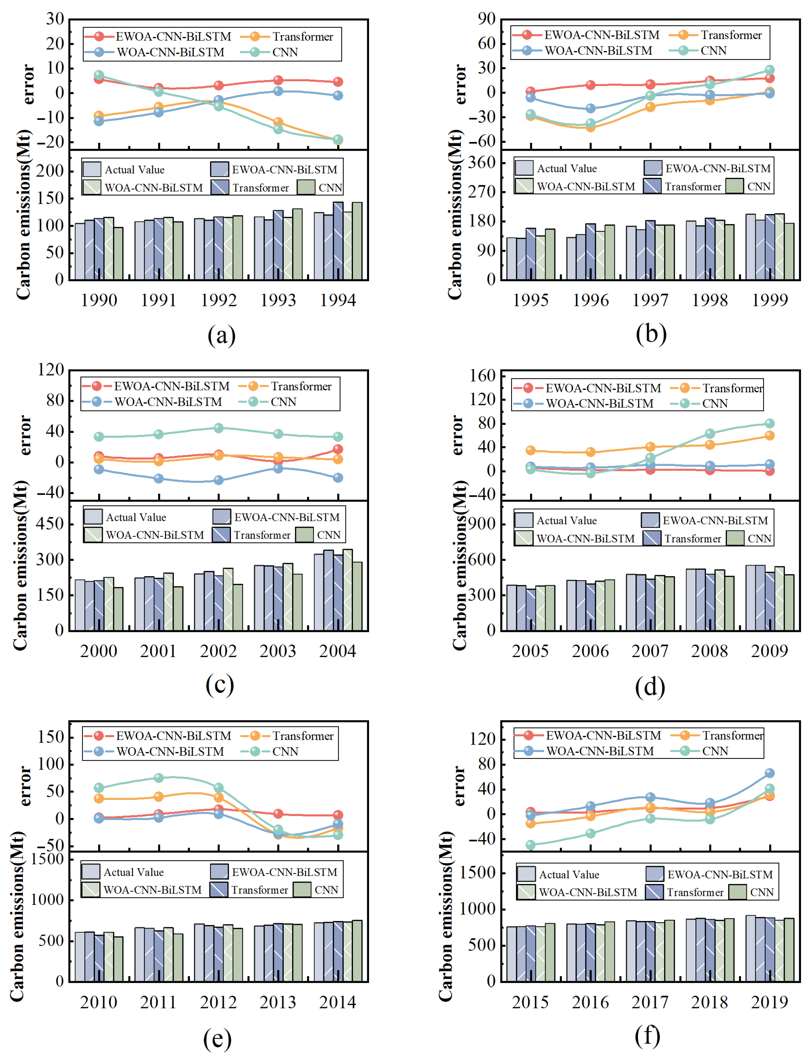
In order to systematically evaluate the adaptability of different machine learning architectures for regional carbon emission prediction, WOA-CNN-BiLSTM, CNN, and Transformer models are constructed in this study for comparison, and r, RMSE, MAE, and MAPE are selected as quantitative metrics, and to avoid the randomness of the experiments, five independent repetitions of experiments are performed and averaged for each model (Table 2 and Figure 7).
EWOA-CNN-BiLSTM maintains optimal performance on both training and test sets, with its test set R 2 (0.9989) close to the theoretical upper limit, and RMSE (8.4962) and MAPE (0.0216) significantly lower than those of the other models, which verifies the synergistic advantage of the hybrid architecture of EWOA and CNN-BiLSTM; the WOA-CNN-BiLSTM training set performs moderately well ( R 2 = 0.9974), but the test set error rises significantly (RMSE = 19.9267, MAPE = 0.1104), revealing local convergence defects in the WOA algorithm. The CNN model lacks the ability of temporal modeling, and the test set has the highest values of both RMSE (32.0286) and MAPE (0.1449), which highlights the limitation of a single convolutional structure in capturing the time-series dynamics of carbon emissions. The MAPE (0.0286) of the Transformer model is significantly lower than that of the CNN (0.1449) on the test set, which indicates that its self-attention mechanism is capable of capturing the global temporal dependence of carbon emission data; however, its RMSE (25.1076) and MAE (21.1504) are significantly worse than that of the EWOA-CNN-BiLSTM (RMSE = 8.4962, MAE = 6.594). In conclusion, EWOA-CNN-BiLSTM is the optimal solution, and the rest of the models need algorithmic improvement for structural defects.

3.4. Scenario Forecasting

3.4.1. Scenario Setting

A scenario is a description of a future situation, or a series of implementation options that may lead the situation from an initial state to a future state. It is not only a theoretical conception, but also a forward-looking insight into the development trend of reality, which can provide a valuable reference direction for decision-making. In this study, four different development scenarios are established by combining the actual situation with relevant policy initiatives and drawing on the research results of related scholars: the baseline scenario (TBS), the green scenario (TGS), the low-carbon scenario (LCS) and the high-carbon scenario (HCS). The four scenarios represent different development paths and possibilities, ranging from the more conservative and traditional to the innovative and transformative, and are useful for comprehensively assessing the future direction and potential impacts of carbon emissions from transportation.
(1)
TBS: The baseline scenario establishes a reference framework based on the current development trajectory and existing policies. In this scenario, the transportation sector will continue its existing growth trend and be strictly implemented in accordance with the existing planning and policies. Driven by the stable growth of the domestic economy and the steady progress of urbanization, the data of various indicators will develop steadily under normal circumstances.
(2)
TGS: Based on the baseline scenario, the implementation of existing development policies is accompanied by increased efforts to implement energy efficiency policies, including the optimization of the transportation environment, the advancement of alternative-energy-powered automobiles and the enhancement of traffic control systems. The green scenario, which emphasizes the qualitative aspects of economic progression and the sustenance of economic expansion, will be slower than in the baseline scenario; however, the energy structure is significantly improved.
(3)
LCS: Under the existing plan, carry out low carbonization construction, adjust the structure of the transport industry, vigorously develop new energy vehicles, build highways and public transport systems, and implement transport-demand management policies to significantly reduce carbon emissions. Compared with the green scenario, the low-carbon scenario places greater emphasis on the qualitative dimensions of economic growth while safeguarding economic growth. By optimizing freight transport modes and improving transport efficiency, as well as transforming the energy structure, key indicators such as freight transport volume, freight transport turnover, and gasoline consumption of the transport industry are expected to show a more positive trend of carbon emission reductions, reflecting a more aggressive attitude of the scenario in advancing sustainable development and environmental improvement.
(4)
HCS: In light of the severe impact of the COVID-19 pandemic on economic development, the prevailing scenario prioritizes economic growth as its main objective, with a concomitant lack of emphasis on low-carbon environmental protection issues. This scenario is characterized by minimal consideration of the structure and modalities of the transportation sector. Furthermore, growth-oriented approaches are prone to increase the demand for transportation, which in turn will significantly increase carbon emissions, posing a considerable challenge to the pursuit of sustainable development.
Informed by the historical datasets of various indicators coupled with an analysis of the present context, and referring to the 14th Five-Year Plan and the long-term goal for 2035, the National Population Development Plan (2016–2030), the 14th Five-Year Comprehensive Energy Conservation and Emission Reduction Plan, and the 14th Five-Year Development Plan for Comprehensive Transportation Services, the growth rates of various indicators are reasonably adjusted (Table 3). The changes in the rate of each variable in the different scenarios are analyzed in detail as follows.
(1)
GDP of the tertiary sector: Currently, the economic trajectory of China has shifted from a phase of rapid economic growth to a stage characterized by high quality advancement, with the rate of economic growth gradually slowing. The outline highlights that China’s economy has entered a new era of development of the 14th Five-Year Plan, defined by a persistent shift and enhancement in the industrial framework, and a steady increase in the share of the tertiary industry within the economic landscape. According to the State Information Center’s forecast of China’s industrial structure, the proportion of tertiary industry is experiencing a steady ascension, with projections indicating that it will reach approximately 58% by the year 2025, 65% by 2030, and 72% by 2035.
(2)
Population: With the aging of the population and changes in fertility concepts, the growth rate of the population in China is expected to maintain a downward trend. The National Population Development Plan (2016–2030) forecasts waning momentum in China’s population growth, with the total population reaching its peak around 2030 and then persistently decreasing.
(3)
Passenger turnover: According to the “14th Five-Year Development Plan for Comprehensive Transportation Services”, passenger travel demand is expected to grow steadily. It is projected that from 2021 to 2025, the average annual growth rate of passenger travel will be approximately 4.3%, with increasing shares of high-speed rail, civil aviation, and private car travel. Therefore, it can be inferred that with the continuous economic growth and the rising popularity of private cars, passenger turnover is expected to continue to rise.
(4)
Freight: Freight transportations is the foundation that supports social and economic development. The “14th Five-Year Development Plan for Comprehensive Transportation Services” indicates that freight demand is stable with a slight increase. It is projected that from 2021 to 2025, the mean annual growth rate for the total freight volume in society will reach 2.3%, indicating a steady but moderate increase in the transportation of goods during that time frame.
(5)
Freight turnover: The outline suggests expediting the evolution of a contemporary, unified transportation network, along with the implementation of supportive policies aimed at enhancing transport efficiency and optimizing the overall transportation infrastructure.
Table 3. Changes in the rate of each variable in different scenarios (%).
YearScenarioX3X6X8X9X11X17
2020–2025TBS60.22342
TGS50.151.52.53.51
LCS40.1123−1
HCS7.50.33453
2026–2030TBS40.12.54.53.5−1
TGS30.05243−1.2
LCS20.11.532.5−1.5
HCS5.50.23.5541
2031–2035TBS2−0.1353−3
TGS1.8−0.152.54.52.5−3.2
LCS1.5−0.2242.2−3.5
HCS3.50.1463.5−1
2036–2040TBS1.8−0.23.55.52.5−3.5
TGS1.5−0.22352.2−3.8
LCS1.2−0.242.54.52−4
HCS2.5−0.14.56.53−2
2041–2045TBS1.5−0.2245.82.2−4
TGS1.2−0.243.55.51.8−4.5
LCS1−0.26351.6−4.8
HCS2−0.2572.5−3
2046–2050TBS1.2−0.244.561.8−5
TGS1−0.2645.81.6−5.5
LCS0.8−0.283.55.51.4−5.8
HCS1.5−0.225.57.52−4
Note: The values represent changes in rates (%). Negative values are indicated with a minus sign.

3.4.2. Situational Analysis

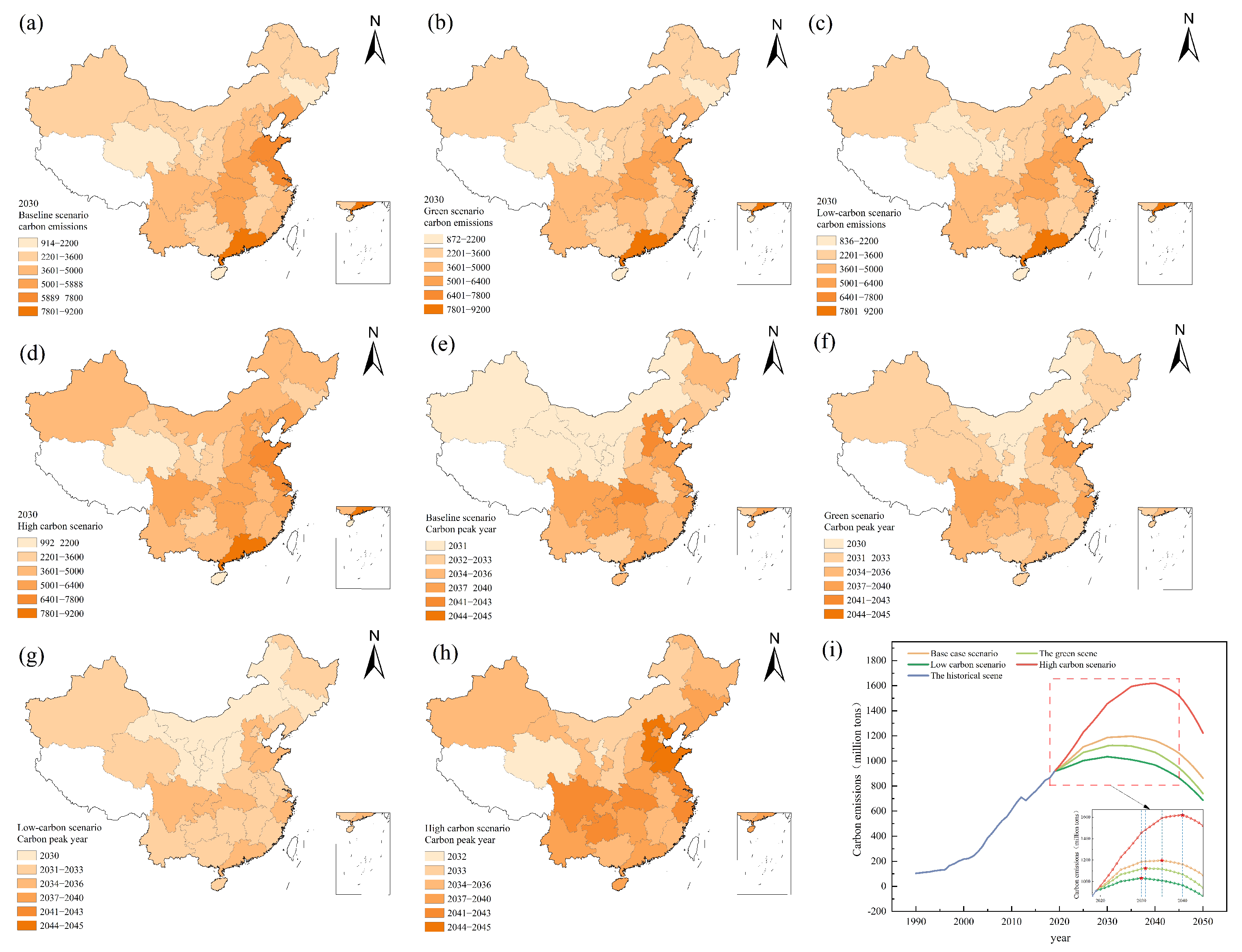
Based on the four scenarios and the different settings of the influencing factor indicators in this study, the TCE forecasting model is used to predict the projected carbon emissions from 2020 to 2050. These four scenarios cover different development paths and policy directions, and can comprehensively and meticulously reflect the various possible situations of carbon emissions in the future transportation sector. By analyzing these projections, we can gain a clear insight into the dynamic changes of carbon emissions over time under different scenarios, thus providing strong data support for the formulation of scientific and reasonable emission reduction policies and sustainable development strategies. (Figure 8).
Under TBS, several western provinces will peak in 2031, and total TCE will peak in 2035, totaling about 1197 million tons, 1.31 times higher than in 2019, which will prevent China from achieving its dual-carbon goals if it develops according to the baseline scenario. Under TGS, provinces such as Neimenggu and Shanxi will take the lead in achieving the carbon peaking target, with overall peaking expected in 2031. Under LCS, most provinces will reach their peak targets by 2030, with an overall peak in 2031 and a peak volume of 1045 million tons. Under HCS, no province will achieve the peak target on time, and the overall peak time is projected to be 2040, with a peak amount of 1619 million tons, which is 422 million tons higher than under TBS. Therefore, pursuing economic growth and neglecting carbon emission reduction will hinder the realization of the dual-carbon target. In conclusion, the peak time is between 2030 and 2040, and all scenarios except the low-carbon scenario are later than the target time. The peak level is between 1100 million tons and 1700 million tons, which is the main source of carbon emissions, so the TCE to achieve the dual-carbon target is of great significance to China’s dual-carbon target.

4. Discussion

This study endeavors to conduct an exhaustive exploration of the determinants affecting TCE and to establish a precise predictive model for carbon emissions. Utilizing the improved LASSO regression model for feature selection, we have determined that the GDP of the tertiary industry, population, passenger turnover, freight, freight turnover, and transportation gasoline consumption are pivotal influencers of TCE in China. Achieving decarbonization in the transportation sector requires an integrated, multidimensional perspective on technology, institutions, and governance. As population size and economic level are less amenable to adjustment, the study suggests focusing on transportation structure optimization, transport efficiency enhancement, clean energy promotion, and policy reinforcement to counteract the impact of these key factors on TCE.
Regarding the construction of a deep learning model, this study has developed an EWOA-CNN-BiLSTM neural network tailored to the spatio-temporal attributes of carbon emissions for accurate prediction. The EWOA-CNN-BiLSTM model has demonstrated marked effectiveness, achieving an R 2 value of 0.9993 on the training dataset, significantly surpassing other models. On the testing dataset, the R 2 value stands at 0.9989, slightly reduced yet maintaining substantial accuracy and reliability. This suggests the model’s ability to effectively capture the spatio-temporal characteristics of carbon emission data, thereby enhancing prediction significance.
According to the research conducted by Chen et al. [36], under a scenario of technological breakthroughs, TCE is projected to peak by 2030, highlighting the significance of technological innovation. In the study by Li et al. [35], it is suggested that the Chinese government should formulate additional supportive policies to drive energy transition, optimize the structure of transportation, and enable TCE to achieve its peak by 2030. In scenario forecasting, China’s TCE will only achieve a peak within the anticipated timeframe under a low-carbon scenario, while all other scenarios will delay peaking until after 2030. Notably, the high-carbon scenario, which accounts for post-pandemic economic recovery, will reach its peak in 2040, far beyond the 2030 target. The study highlights the importance of placing a high priority on carbon emission reduction while pursuing economic growth.

5. Conclusions and Policy Implications

5.1. Conclusions

This study initially uses the improved LASSO regression model to meticulously filter and discern the primary drivers that contribute to TCE, and then constructs an EWOA-CNN-BiLSTM model to predict the peak TCE under four set scenarios, yielding the following key conclusions:
(1)
TCE grows rapidly between 1990–2019. In the time dimension, TCE is fluctuating and rising, with emissions surging from 104 million tons to 916 million tons. In terms of spatial distribution, China’s carbon emissions show a pattern of high in the east and low in the west, high in the south and low in the north, and the gap is widening year by year.
(2)
This study utilizes the improved LASSO regression technique to screen and analyze the critical factors influencing TCE. The findings indicate that the six most significant factors, in descending order, are GDP of the tertiary sector, population, passenger turnover, freight, freight turnover, and transportation gasoline consumption.
(3)
Across diverse scenarios, under different circumstances, the time and magnitude of the peak TCE vary. Under TBS and TGS, the peak is expected in 2030–2040, posterior to the national target for the carbon peak. Under HCS, the peak is projected to occur in 2040, with emissions in this scenario substantially exceeding those in other scenarios, posing significant challenges to China’s “dual-carbon” objectives.
(4)
Compared with other scenarios, the TCE in the low-carbon emission scenario is significantly lower. TCE is expected to peak in 2030 at 1045 million tons, and by 2050, there will be a negative growth rate relative to 2021, and hopefully carbon neutrality will be achieved by 2060. This scenario is most conducive to the sustainable development of China’s transportation sector. China should formulate low-carbon policies, strengthen the promotion of clean energy, and optimize its transportation structure to facilitate the early realization of dual-carbon goals in the transport sector.
However, there are still some limitations in this study, as different scholars choose different variables to characterize TCE and determine different prediction models, which leads to different conclusions on the timing and peak value of the carbon peak. Such differences not only increase the uncertainty of carbon emission research results, but also bring challenges to policymakers in formulating scientific and effective emission reduction policies based on the research results. In view of this, subsequent studies should focus on further exploring the selection of key TCE variables and exploring more accurate TCE prediction methods.

5.2. Policy Implications

Based on the research findings of TCE prediction in this paper, the following policy recommendations are put forward to promote the low-carbon development of the transportation industry.
(1)
Widespread implementation of clean energy and low-carbon technologies. Support the research and development of new energy vehicles (NEVs) and their promotion [37], enhance subsidies and incentives for the purchase of NEVs, and encourage enterprises and consumers to buy and use low-carbon transportation options [38]. Improve the infrastructure for charging stations and battery swapping stations to facilitate the popularization of NEVs. Optimize the public transportation system to enhance its convenience and attractiveness, guiding the public to choose public transportation for commuting.
(2)
Strengthening the green construction and intelligent upgrading of transportation infrastructure. In the construction or renovation of transportation infrastructure, adopt green, low-carbon, and environmentally friendly design concepts, and use sustainable building materials such as green concrete to reduce carbon emissions during the construction and operation phases [39]. Promote the use of renewable energy technologies in transportation infrastructure to provide green energy for road lighting and traffic signal systems. Spread the use of intelligent transportation facilities, such as smart traffic signals and intelligent parking lots, to increase the performance of the transportation system while decreasing energy expenditure.
(3)
Enhancing carbon emission regulation and incentive measures. Develop targeted carbon emission control policies and establish a comprehensive system for carbon emission monitoring, reporting, and verification to ensure the authenticity and transparency of corporate carbon emission data. Provide tax incentives and financial subsidies for the research, development, and application of low-carbon technologies [40], encouraging enterprises to reduce carbon emissions and achieve sustainable development in the transportation industry.

Author Contributions

Conceptualization, Y.S., K.L. and Q.L.; methodology, Y.S.; software, K.L.; validation, Y.S., K.L. and Q.L.; formal analysis, Y.S.; investigation, Y.S.; resources, Y.S., K.L. and Q.L.; data curation, K.L.; writing—original draft preparation, Y.S.; writing—review and editing, Y.S. and Q.L.; visualization, Y.S. and K.L.; supervision, Y.S.; project administration, Y.S. and Q.L.; funding acquisition, Y.S. and Q.L. All authors have read and agreed to the published version of the manuscript.

Funding

This study was funded by the Natural Science Foundation of Shandong Province (Grant No. ZR2021MG021) and the Youth Innovation Technology Project of Higher School in Shandong Province (Grant No. 2021RW030).

Institutional Review Board Statement

Not applicable.

Informed Consent Statement

Not applicable.

Data Availability Statement

Restrictions apply to the availability of these data. Data was obtained from China Statistics Bureau and are available China Statistics Bureau with the permission of China Statistics Bureau.

Conflicts of Interest

The authors declare no conflicts of interest.

References

  1. Qin, X.; Xu, X.; Yang, Q. Carbon peak prediction and emission reduction pathways of China’s low-carbon pilot cities: A case study of Wuxi city in Jiangsu province. J. Clean. Prod. 2024, 447, 141385. [Google Scholar] [CrossRef]
  2. Li, F.; Cai, B.; Ye, Z.; Wang, Z.; Zhang, W.; Zhou, P.; Chen, J. Changing patterns and determinants of transportation carbon emissions in Chinese cities. Energy 2019, 174, 562–575. [Google Scholar] [CrossRef]
  3. Sun, Y.; Yang, Y.; Liu, S.; Li, Q. Research on transportation carbon emission peak prediction and judgment system in China. Sustainability 2023, 15, 14880. [Google Scholar] [CrossRef]
  4. Wang, X.; Zhou, Y.; Bi, Q.; Cao, Z.; Wang, B. Research on the low-carbon development path and policy options of China’s transportation under the background of dual carbon goals. Front. Environ. Sci. 2022, 10, 905037. [Google Scholar] [CrossRef]
  5. Bai, C.; Chen, Z.; Wang, D. Transportation carbon emission reduction potential and mitigation strategy in China. Sci. Total Environ. 2023, 873, 162074. [Google Scholar] [CrossRef]
  6. Zhao, Y.; Duan, X.; Yu, M. Calculating carbon emissions and selecting carbon peak scheme for infrastructure construction in Liaoning Province, China. J. Clean. Prod. 2023, 420, 138396. [Google Scholar] [CrossRef]
  7. Sun, Y.; Zhang, G. Analysis of the measurement of transportation carbon emissions and the emission reduction path in the Yangtze River economic belt under the background of “dual carbon” goals. Energies 2024, 17, 3364. [Google Scholar] [CrossRef]
  8. Zhang, P.; Li, S. Driving factors and scenario prediction of carbon emission from transport sector in the Yangtze River Basin of China. Front. Ecol. Evol. 2023, 11, 1283605. [Google Scholar] [CrossRef]
  9. Luo, X.; Liu, C.; Zhao, H. Driving factors and emission reduction scenarios analysis of CO2 emissions in Guangdong-Hong Kong-Macao Greater Bay Area and surrounding cities based on LMDI and system dynamics. Sci. Total Environ. 2023, 870, 161966. [Google Scholar] [CrossRef]
  10. Zhang, H.; Kong, X.; Ren, C. Influencing factors and forecast of carbon emissions from transportation-Taking Shandong province as an example. IOP Conf. Ser. Earth Environ. Sci. 2019, 300, 032063. [Google Scholar] [CrossRef]
  11. Lin, B.; Xie, C. Reduction potential of CO2 emissions in China’s transport industry. Renew. Sustain. Energy Rev. 2014, 33, 689–700. [Google Scholar] [CrossRef]
  12. Guo, Y.; Hou, Z.; Fang, Y.; Wang, Q.; Huang, L.; Luo, J.; Shi, T.; Sun, W. Forecasting and Scenario Analysis of Carbon Emissions in Key Industries: A Case Study in Henan Province, China. Energies 2023, 16, 7103. [Google Scholar] [CrossRef]
  13. Li, Y.; Dai, J.; Zhang, S.; Cui, H. Dynamic prediction and driving factors of carbon emission in Beijing, China, under carbon neutrality targets. Atmosphere 2023, 14, 798. [Google Scholar] [CrossRef]
  14. Janhuaton, T.; Ratanavaraha, V.; Jomnonkwao, S. Forecasting Thailand’s Transportation CO2 Emissions: A Comparison among Artificial Intelligent Models. Forecasting 2024, 6, 462–484. [Google Scholar] [CrossRef]
  15. Liu, Z.; Han, L.; Liu, M. Spatiotemporal characteristics of carbon emissions in Shaanxi, China, during 2012–2019: A machine learning method with multiple variables. Environ. Sci. Pollut. Res. 2023, 30, 87535–87548. [Google Scholar] [CrossRef] [PubMed]
  16. Liu, B.; Wang, S.; Liang, X.; Han, Z. Carbon emission reduction prediction of new energy vehicles in China based on GRA-BiLSTM model. Atmos. Pollut. Res. 2023, 14, 101865. [Google Scholar] [CrossRef]
  17. Huang, H.; Wu, X.; Cheng, X. The prediction of carbon emission information in Yangtze river economic zone by deep learning. Land 2021, 10, 1380. [Google Scholar] [CrossRef]
  18. Ekaterina, G.; Li, J. Analysis of decarbonization path in New York state and forecasting carbon emissions using different machine learning algorithms. Carbon Neutrality 2024, 3, 8. [Google Scholar] [CrossRef]
  19. Iftikhar, H.; Khan, M.; Żywiołek, J.; Khan, M.; López-Gonzales, J.L. Modeling and forecasting carbon dioxide emission in Pakistan using a hybrid combination of regression and time series models. Heliyon 2024, 10, e33148. [Google Scholar] [CrossRef]
  20. Cansiz, O.F.; Unsalan, K.; Unes, F. Prediction of CO2 emission in transportation sector by computational intelligence techniques. Int. J. Glob. Warm. 2022, 27, 271–283. [Google Scholar] [CrossRef]
  21. Mujeeb, S.; Javaid, N. Deep learning based carbon emissions forecasting and renewable energy’s impact quantification. IET Renew. Power Gener. 2023, 17, 873–884. [Google Scholar] [CrossRef]
  22. Lu, X.; Ota, K.; Dong, M.; Yu, C.; Jin, H. Predicting transportation carbon emission with urban big data. IEEE Trans. Sustain. Comput. 2017, 2, 333–344. [Google Scholar] [CrossRef]
  23. Mao, C.; Luo, J.; Jiao, S.; Zhao, B. Logarithmic Mean Divisia Index Analysis and Dynamic Back Propagation Neural Network Prediction of Transport Carbon Emissions in Henan Province. Energies 2025, 18, 1630. [Google Scholar] [CrossRef]
  24. Sun, Y.; Liu, S.; Li, L. Grey correlation analysis of transportation carbon emissions under the background of carbon peak and carbon neutrality. Energies 2022, 15, 3064. [Google Scholar] [CrossRef]
  25. Tang, J.; Gong, R.; Wang, H.; Liu, Y. Scenario analysis of transportation carbon emissions in China based on machine learning and deep neural network models. Environ. Res. Lett. 2023, 18, 064018. [Google Scholar] [CrossRef]
  26. Xing, Z.; Tan, H.; Zhong, W.; Shi, L. CALMS: Constrained Adaptive Lasso with Multi-directional Signals for latent networks reconstruction. Neurocomputing 2025, 630, 129545. [Google Scholar] [CrossRef]
  27. Duan, L.; Fung, P.L.; Fu, Q.; Chen, J.; Huo, J.; Huang, K.; Wang, G.; Zaidan, M.A.; Guo, Z.; Hussein, T. A robust black carbon prediction model derived from observational datasets in the Yangtze River Delta region, China. Environ. Pollut. 2025, 377, 126361. [Google Scholar] [CrossRef]
  28. Hu, X.; Bai, R.; Li, C.; Shi, B.; Wang, H. Correlations between an Urban Three-Dimensional Pedestrian Network and Service Industry Layouts Based on Graph Convolutional Neural Networks: A Case Study of Xinjiekou, Nanjing. Land 2024, 13, 1553. [Google Scholar] [CrossRef]
  29. Faruque, M.O.; Rabby, M.A.J.; Hossain, M.A.; Islam, M.R.; Rashid, M.M.U.; Muyeen, S. A comparative analysis to forecast carbon dioxide emissions. Energy Rep. 2022, 8, 8046–8060. [Google Scholar] [CrossRef]
  30. Ren, X.; Zhao, B.; Ren, Z.; Xiong, B. Ionospheric TEC Prediction in China during Storm Periods Based on Deep Learning: Mixed CNN-BiLSTM Method. Remote Sens. 2024, 16, 3160. [Google Scholar] [CrossRef]
  31. Jiang, T.; Zheng, C.; Wang, H.; You, S.; Zhang, H.; Wang, Y.; Sun, J.; Wu, Z.; Zhao, W.; Zheng, J. Evaporation temperature prediction of the refrigerant-direct convective-radiant cooling system based on LSTM neural network. Appl. Therm. Eng. 2025, 258, 124693. [Google Scholar] [CrossRef]
  32. Wang, C.; Wang, J.; Ma, L.; Jia, M.; Chen, J.; Shao, Z.; Chen, N. Prediction Modeling and Driving Factor Analysis of Spatial Distribution of CO2 Emissions from Urban Land in the Yangtze River Economic Belt, China. Land 2024, 13, 1433. [Google Scholar] [CrossRef]
  33. Zhang, H.; Li, J.; Yang, H. Cloud computing load prediction method based on CNN-BiLSTM model under low-carbon background. Sci. Rep. 2024, 14, 18004. [Google Scholar] [CrossRef]
  34. Dib, A.; Balac, M.; Sciarretta, A. Deep learning approach to predict microscopic pollutant emissions from mesoscopic traffic simulations. Transp. Res. Part D Transp. Environ. 2025, 146, 104791. [Google Scholar] [CrossRef]
  35. Li, C.; Zhang, Z.; Wang, L. Carbon peak forecast and low carbon policy choice of transportation industry in China: Scenario prediction based on STIRPAT model. Environ. Sci. Pollut. Res. 2023, 30, 63250–63271. [Google Scholar] [CrossRef]
  36. Chen, T.; Wang, M. Deep learning-based carbon emission forecasting and peak carbon pathways in China’s logistics industry. Sustainability 2024, 16, 1826. [Google Scholar] [CrossRef]
  37. Liu, J.; Luo, Y.; Zhu, Q.; Li, Y.; Luo, Y. Research on carbon emission characteristics and mitigation pathways in the vehicle fuel cycle: A case study of Guangdong province. Atmosphere 2023, 15, 3. [Google Scholar] [CrossRef]
  38. Zeng, S.; Ji, M.; Huang, X. An empirical study on the impact of tax incentives on the development of new energy vehicles: Case of China. Energy Policy 2025, 198, 114452. [Google Scholar] [CrossRef]
  39. Xiang, T.; Bian, J.; Li, Y.; Gu, Y.; Wang, Y.; Zhang, Y.; Wang, J. Seasonal Contributions and Influencing Factors of Urban Carbon Emission Intensity: A Case Study of Tianjin, China. Atmosphere 2024, 15, 947. [Google Scholar] [CrossRef]
  40. Zhao, D.; Zhao, M.; Sun, X.; Zhang, H.; Liu, H.; Wu, J.; Lei, Z.; Li, J.; Qian, B.; Lu, L.; et al. Research on Green and Low-Carbon Development Path of China’s Automotive Industry. Chin. J. Urban Environ. Stud. 2023, 11, 2350004. [Google Scholar] [CrossRef]
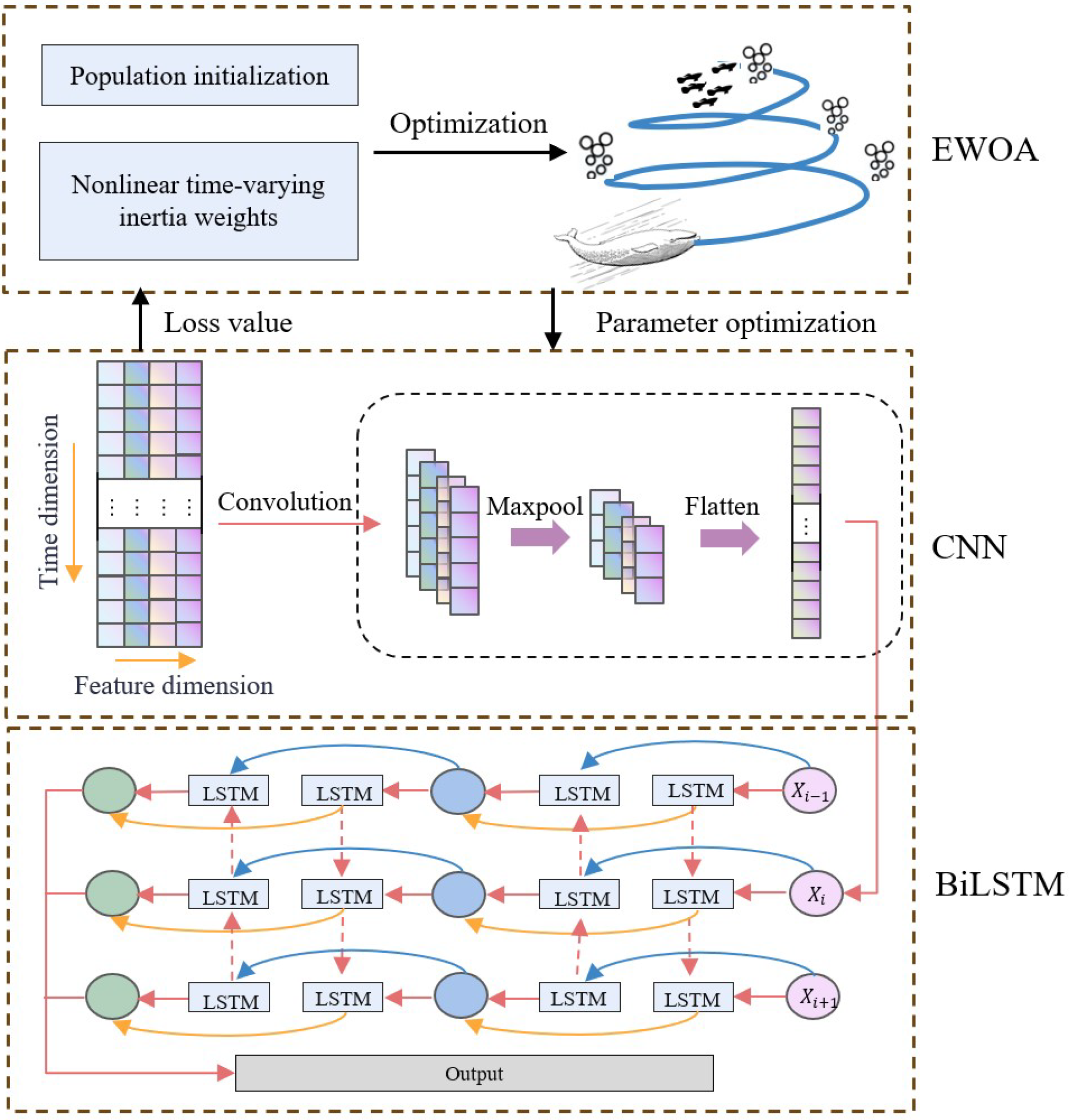
Figure 1. EWOA-CNN-BiLSTM model structure diagram.
Sustainability 17 07102 g001
Figure 2. Research flow chart.
Sustainability 17 07102 g002
Figure 3. Spatial and temporal distribution of TCE. (a) 2005 TCE values for each province in China; (b) 2010 TCE values for each province in China; (c) 2019 TCE values for each province in China; (d) TCE values in China from 1990 to 2019.
Sustainability 17 07102 g003
Figure 4. (a) LASSO model error curve; (b) LASSO regression trajectory.
Sustainability 17 07102 g004
Figure 5. Specific value and correlation analysis. (a) Correlation analysis of key variables; (b) Historical data for key variables.
Sustainability 17 07102 g005
Figure 6. (a) Convergence performance comparison of optimization algorithms; (b) model fitness curve value; (c) the model training set predicts the results; (d) the model test set prediction results.
Sustainability 17 07102 g006
Figure 7. Comparison of model predictions. (a) Comparison of predictions and error maps for each model from 1990 to 1994; (b) Comparison of predictions and error maps for each model from 1995 to 1999; (c) Comparison of predictions and error plots for each model from 2000 to 2004; (d) Comparison of predictions and error plots for each model from 2005 to 2009; (e) Comparison of predictions and error plots for each model from 2010 to 2014; (f) Comparison of predictions and error plots for each model from 2015 to 2019.
Sustainability 17 07102 g007
Figure 8. Carbon emission projection results and time to peak. (a) Baseline scenario for TCE in each province in 2030; (b) Green scenario for TCE in each province in 2030; (c) Low-carbon scenario for TCE in each province in 2030; (d) High carbon scenario for TCE in each province in 2030; (e) Peak carbon year for each province in the baseline scenario; (f) Peak carbon year for each province in the Green scenario; (g) Peak carbon year for each province in the low-carbon scenario; (h) Peak carbon year for each province in the High carbon scenario; (i) TCE values by scenario.
Sustainability 17 07102 g008
Table 1. Factors affecting transportation carbon emissions.
DimensionVariableSymbol
Economic indicatorsGDP of the primary sectorX1
GDP of the secondary sectorX2
GDP of the tertiary sectorX3
GDPX4
Demographic scaleGross domestic product per capitaX5
PopulationX6
Transport capacityPassenger trafficX7
Passenger turnoverX8
FreightX9
Transport turnoverX10
Freight turnoverX11
Societal factorsUrbanization rateX12
Total industrial output valueX13
Civil vehicle ownershipX14
Number of transport practitionersX15
Energy compositionTransport power balance sheetX16
Transportation gasoline consumptionX17
Electricity consumption in the transport industryX18
Table 2. Error coefficients for each model.
SampleIndicatorEWOA-CNN-BiLSTMWOA-CNN-BiLSTMARIMATransformer
Training set R 2 0.99930.99740.98430.9728
MAE6.196810.580532.902520.0945
MAPE0.02290.03690.17120.0852
RMSE7.441713.830736.511226.3581
Testing set R 2 0.99890.99390.97620.9771
MAE6.59417.862635.078321.1504
MAPE0.02160.11040.11960.0286
RMSE8.496219.926739.062525.1076
Disclaimer/Publisher’s Note: The statements, opinions and data contained in all publications are solely those of the individual author(s) and contributor(s) and not of MDPI and/or the editor(s). MDPI and/or the editor(s) disclaim responsibility for any injury to people or property resulting from any ideas, methods, instructions or products referred to in the content.