Multi-Objective Scheduling Method for Integrated Energy System Containing CCS+P2G System Using Q-Learning Adaptive Mutation Black-Winged Kite Algorithm

Abstract

This study proposes an improved multi-objective black-winged kite algorithm (MOBKA-QL) integrating Q-learning with adaptive mutation strategies for optimizing multi-objective scheduling in integrated energy systems (IES). The algorithm dynamically selects mutation strategies through Q-learning to enhance solution diversity and accelerate convergence. First, an optimal scheduling model is established, incorporating a carbon capture system (CCS), power-to-gas (P2G), solar thermal, wind power, and energy storage to minimize economic costs and carbon emissions while maximizing energy efficiency. Second, the heat-to-power ratio of the cogeneration system is dynamically adjusted according to load demand, enabling flexible control of combined heat and power (CHP) output. The integration of CCS+P2G further reduces carbon emissions and wind curtailment, with the produced methane utilized in boilers and cogeneration systems. Hydrogen fuel cells (HFCs) are employed to mitigate cascading energy losses. Using forecasted load and renewable energy data from a specific region, dispatch experiments demonstrate that the proposed system reduces economic costs and CO₂ emissions by 14.63% and 13.9%, respectively, while improving energy efficiency by 28.84%. Additionally, the adjustable heat-to-power ratio of CHP yields synergistic economic, energy, and environmental benefits.

1. Introduction

With socioeconomic development, population growth, and rising living standards, the demand for electricity, heating, and cooling resources has surged, while traditional fossil energy reserves are progressively depleting [1]. Renewable energy sources (e.g., wind and solar power) have emerged as essential alternatives to fossil fuels due to their cleanliness, sustainability, and cost-effectiveness [2,3]. CHP systems, recognized for their high efficiency, low-carbon footprint, and energy-saving potential, are widely adopted in modern power systems to simultaneously generate electricity and utilize waste heat [4]. Recently, the integration of fossil fuel-based integrated energy systems (IES) with renewable energy has garnered significant attention, as it enhances energy diversity while reducing carbon emissions [5]. However, the operational complexity of IES—driven by diverse equipment and dynamic conditions [6]—necessitates strategic optimization to ensure efficient performance [7]. To address this challenge, this study proposes an intelligent optimization algorithm that combines Q-learning with adaptive mutation strategies. The proposed approach aims to resolve the multi-device coordination and coupling issues in IES and improve overall operational efficiency and energy utilization.

1.1. Literature Review

In IES, pollutant emissions primarily originate from fossil fuel-based equipment. Integrating renewable energy (e.g., solar/wind) and clean technologies is critical for emission reduction. Zhang et al. [8,9,10] demonstrated that incorporating solar and wind power into IES not only alleviates supply–demand imbalances and climate impacts but also enhances economic performance by minimizing energy waste through wind curtailment utilization. However, the inherent intermittency of renewables remains a research challenge. Addressing this, Karolina et al. [11] developed a hydrogen storage solution using electrolysis for stable energy recovery.

Recent studies have demonstrated that integrating energy conversion and storage devices significantly enhances system performance. Li et al. [12] proposed a two-layer alternating optimization dispatch model incorporating CCS systems, quantifying both economic benefits and carbon emission reductions. Chen et al. [13,14,15] implemented P2G technology, utilizing surplus electricity for water electrolysis to produce hydrogen, which subsequently reacted with CO₂ captured by CCS to synthesize methane. Their approach incorporated hydrogen storage devices and HFC to effectively reduce energy cascade losses. For renewable energy management, Marco et al. [16] verified that battery energy storage systems effectively mitigate renewable generation and load fluctuations. Through comparative scenario analysis, Rakibul et al. [17] established that a thermal energy storage tank (TES) combined with excess energy recovery could increase renewable energy penetration while reducing carbon emissions. As a core component of IES, CHP systems require the coordinated optimization of both equipment design and operational strategies. Common strategies such as following electric load (FEL) and following thermal load (FTL) exhibit scenario-dependent performance variations. Song et al. [18] systematically evaluated CHP operation strategies, emphasizing that optimal strategy selection is critical for maximizing system efficiency.

The integration of multiple devices significantly increases the coupling complexity of Integrated Energy Systems (IES). To efficiently obtain optimal solutions under complex constraints, intelligent optimization algorithms have been increasingly adopted in IES scheduling problems. Commonly used algorithms include the sparrow search algorithm (SSA) [19], genetic algorithm (GA) [20], and whale optimization algorithm (WOA) [21]. Recent advancements have focused on incorporating multi-objective optimization mechanisms and adaptive mutation strategies to enhance global search capability and solution diversity. For instance, Li et al. [22] proposed the MOAOA algorithm, which integrates non-dominated sorting and mutation operations to effectively optimize the system configuration in multi-objective scenarios. Algorithmic improvements often focus on the design of mutation strategies. Yu et al. [23] employed a time-varying Gaussian mutation strategy to address the loss of population diversity in the later stages of Particle Swarm Optimization (PSO). Li et al. [24] developed the Improved Dung Beetle Optimizer (IDBO) based on an adaptive t-distribution, which significantly enhanced both the optimization performance and search accuracy. While these methods demonstrate effective solution space exploration through distinct mutation strategies, most still employ static, predefined mechanisms without real-time environmental interaction.

In recent years, deep reinforcement learning (DRL) has demonstrated significant potential for IES modeling and scheduling owing to its strong generalization capabilities and adaptability to complex environments. Dong et al. [25] developed a soft actor–critic (SAC) algorithm and built an environmental interaction model to simulate real-time feedback for DRL training. Suo et al. [26,27] employed deep learning to reduce modeling complexity and uncertainty in IES, significantly enhancing algorithmic computational efficiency. Chen et al. [28,29] implemented Q-learning for energy management optimization, improving both sample efficiency and generalization ability. As a model-free reinforcement learning method, Q-learning dynamically learns optimal strategies through environmental interaction. When integrated into mutation selection processes, it facilitates adaptive strategy adjustment based on real-time search-state feedback, thereby effectively balancing global exploration and local exploitation.

The black-winged kite algorithm (BKA), proposed by Wang et al. in 2024 [30], is a novel metaheuristic optimization method inspired by the migratory and predatory behaviors of black-winged kites. This algorithm innovatively integrates a Cauchy mutation strategy with a leader-following mechanism. Comprehensive benchmark tests have demonstrated its effectiveness in solving constrained optimization problems. Given these advantages, we adopt BKA in this study to ensure reliable and efficient energy management in integrated energy systems.

1.2. Research Gap

(1) Existing studies have rarely integrated energy storage and conversion units—including renewable energy sources, CCS, P2G systems, and oxygen storage tanks (OST)—into a unified IES. Furthermore, the selection of CHP operation strategies, which critically impacts IES performance, often lacks synergistic coordination with equipment configurations. Most current approaches adopt fixed heat-to-power ratio strategies while failing to accommodate dynamic variations in system load fluctuations and energy demands, thereby constraining system adaptability.

(2) Current heuristic optimization methods for IES scheduling frequently exhibit premature convergence and slow convergence rates, largely attributable to static mutation mechanisms. Although Q-learning has demonstrated potential in energy management applications, its implementation has been restricted to policy-level optimization without integration into mutation operations. This limitation results in insufficient autonomous learning capacity, compromising adaptability in dynamic operating conditions. Moreover, critical multi-objective evaluation metrics (e.g., hypervolume (HV), the multi-objective value index (MOVI)) remain underutilized, highlighting persistent challenges in multi-objective optimization.

1.3. Research Contribution

A review of the literature on the optimal dispatch of IES reflects that coupling wind and solar energy with these systems has become essential. The introduction of the CCS+P2G system can significantly improve system operating efficiency, reduce carbon emissions, curtail the common wind power curtailment phenomenon, and reinforce system stability and reliability. The CHP system with an adjustable heat-to-power ratio can flexibly adapt to demand, optimize electric and heat output, strengthen efficiency, and lower costs. The introduction of an OST has enhanced oxyfuel combustion and diminished natural gas consumption. To address the complexity of a multi-variable IES, this paper proposes a MOBKA-QL algorithm with adaptive variation, which leverages Q-learning to interact with the environment and enhance optimization performance.

Therefore, the main research contributions of this paper are drawn as follows:

(1)

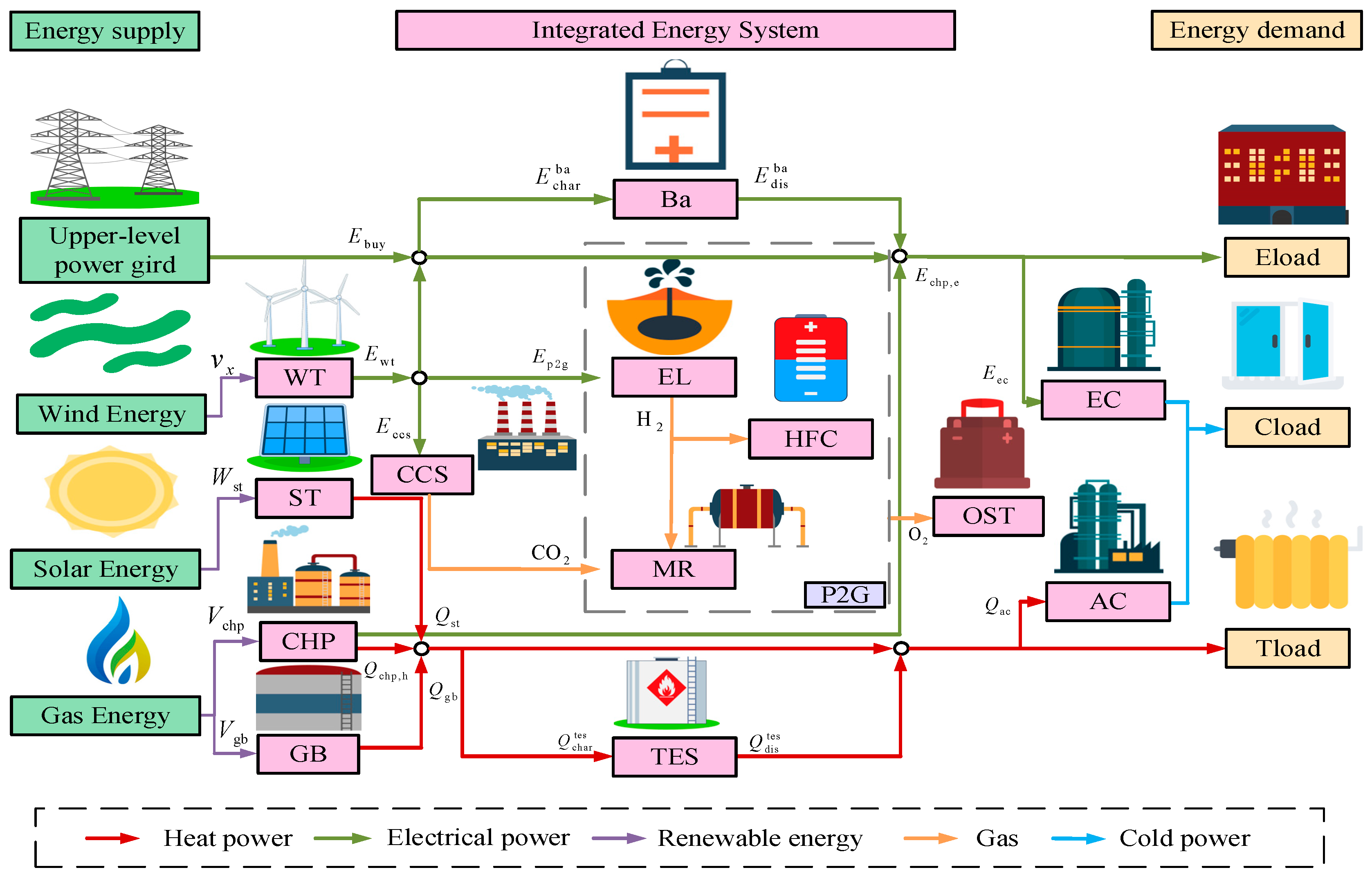
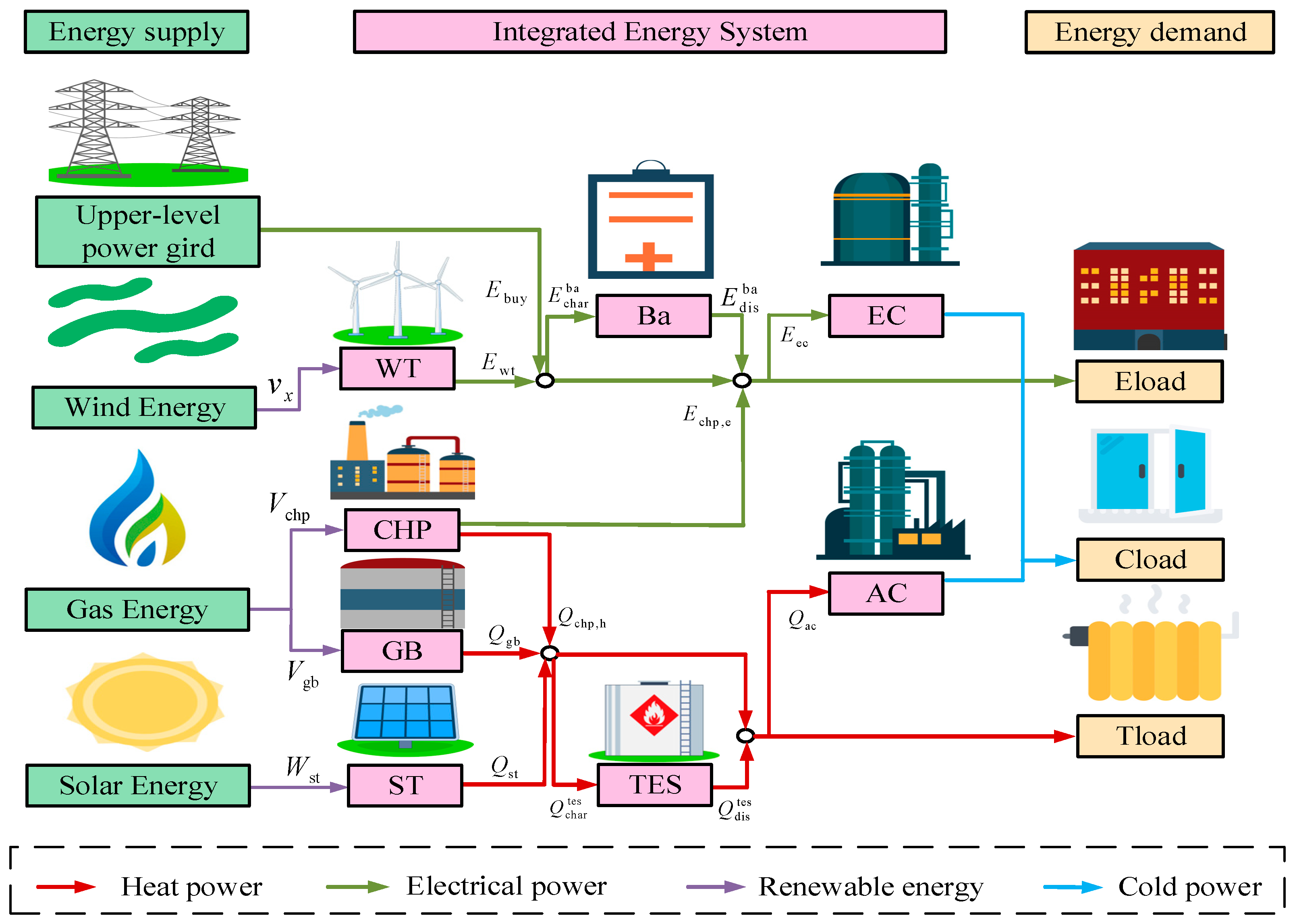
A multi-objective optimal scheduling model for the IES was established, aiming to minimize economic cost and CO₂ emissions while maximizing energy efficiency. The IES integrates multiple energy conversion and storage devices, involving technologies such as power generation, energy storage, gas production, and CCS. It can efficiently satisfy the combined load demand for power, heat, and cooling.

(2)

MOBKA-QL integrates five mutation strategies and employs Q-learning for adaptive selection during iterations, enabling environment-aware and self-learning capabilities. The original BKA is extended to handle multi-objective optimization. In this framework, solution sets are first evaluated by MOVI, then ranked based on crowding distance, and finally, the optimal Pareto solution is selected using TOPSIS, making it well-suited for IES scheduling.

(3)

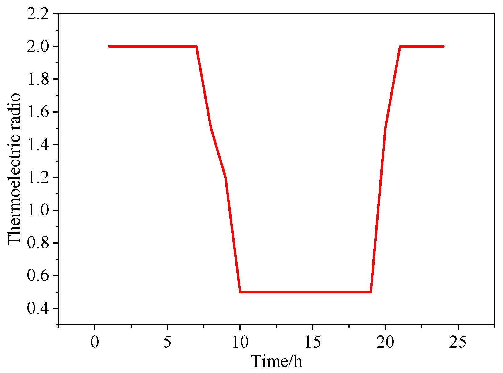
The operation of CHP adopts an adjustable heat-to-power ratio strategy, which combines real-time data on demand-side loads and renewable energy to dynamically adjust energy supply. Using the same algorithm and model, we compared this strategy with a constant heat-to-power ratio strategy in a test, which verified the superiority of the former in terms of economy, environment, and energy.

The rest of this paper is organized as follows. Section 2 describes the structure and mathematical model of IES. Section 3 presents MOBKA-QL and the scheduling model of IES. In Section 4, the performance of the algorithms is tested, as well as energy utilization, economic benefits, the environmental benefits of IES, and the choice of CHP thermoelectric ratio strategy through a typical season; optimization experiments are conducted in different scenarios. The results are analyzed and discussed in Section 5.

2. Integrated Energy System Modeling

The internal energy demand of the IES was addressed through the coordinated integration of diverse energy sources and supply equipment. An extended CCS model is proposed in this study, improving upon conventional frameworks. As illustrated in Figure 1, the study focuses on the efficient utilization of hydrogen energy, the adjustable heat-to-power ratio of CHP systems, and the power equipment involved in the two-stage P2G conversion process.

As illustrated in Figure 1, the IES proposed in this study comprises wind turbines, CHP units, solar collector panels, and gas boilers to supply energy for overall system operation. On the demand side, the system accommodates thermal, electrical, and cooling loads. The cooling load is met by an absorption chiller (AC) and an electric chiller (EC). The intermediate energy conversion and storage infrastructure includes a carbon capture unit, a heat storage tank, a battery, an OST, and a two-stage P2G unit. The P2G system generates hydrogen for HFC, which supplies electricity to the system. This setup facilitates the decoupling of heat and power, thereby improving operational flexibility and enabling better utilization of wind power. The integration of CCS with P2G technology reduces system emissions and mitigates wind power curtailment while supplying natural gas, electricity, and heat. Additionally, the oxygen produced during the two-stage P2G process is stored in oxygen tanks and supplied to CHP units for oxygen-enriched combustion, which decreases natural gas consumption, lowers costs, and enhances overall system efficiency.

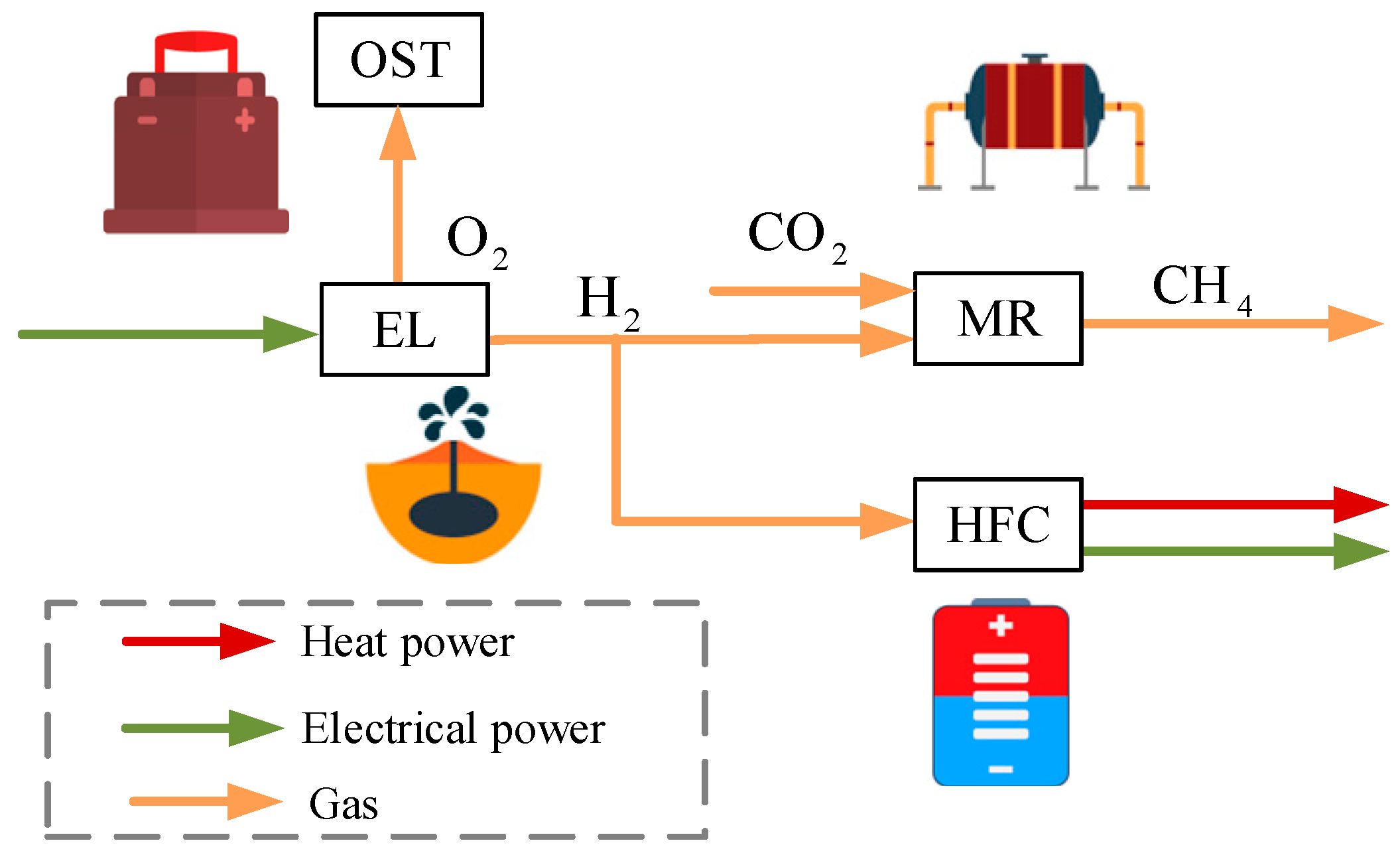
2.1. Two-Stage P2G Operational Process

Hydrogen energy, recognized for its purity and efficiency, holds significant potential across various applications, such as hydrogen-powered vehicles and hydrogen fuel cells [31]. The two-stage operation process of P2G is illustrated in Figure 2.

In the two-stage P2G system, the direct utilization of HFCs reduces energy losses associated with multi-step conversions compared to the conventional methanation reaction (MR) pathway. Additionally, an OST is incorporated into the P2G model to store oxygen generated via water electrolysis and supply it to the CHP unit for oxyfuel combustion, thereby reducing the unit’s reliance on natural gas. The corresponding energy conversion process is formulated as follows.

(1)

Electrolytic cell

$$\left\{\begin{array}{l}{W}_{{\mathrm{el},\mathrm{H}}_2,t}={\eta }_{\mathrm{el}}{E}_{e,\mathrm{EL},t}\\ E_{e,\mathrm{el}}^{\min }\le E_{e,\mathrm{el},t}\le E_{e,\mathrm{el}}^{\max }\\ \mathsf{\Delta }{E}_{e,\mathrm{el}}^{\min }\le E_{e,\mathrm{el},t+1}-E_{e,\mathrm{el},t}\le \mathsf{\Delta }{E}_{e,\mathrm{el}}^{\max }\end{array}\right.$$

(1)

where $E_{e,\mathrm{el},t}$ represents the electrical energy input to the electrolytic cell (EL) in time period t; $W_{{\mathrm{el},\mathrm{H}}_2,t}$ denotes the hydrogen energy output from the EL in time period t; ${\eta }_{el}$ indicates the energy conversion efficiency of the EL; $E_{e,\mathrm{el}}^{\max }$ and $E_{e,\mathrm{EL}}^{\min }$ specify the upper and lower limits of the electrical energy input to the EL, respectively; and $\mathsf{\Delta }{E}_{e,\mathrm{el}}^{\max }$ and $\mathsf{\Delta }{E}_{e,\mathrm{el}}^{\max }$ refer to the upper and lower limits of the climb of the EL, respectively.

(2)

Methane reactor

$$\left\{\begin{array}{l}{W}_{\mathrm{mr},g,t}={\eta }_{\mathrm{mr}}{W}_{{\mathrm{H}}_2,\mathrm{mr},t}\\ W_{{\mathrm{H}}_2,\mathrm{mr}}^{\min }\le W_{{\mathrm{H}}_2,\mathrm{mr},t}\le W_{{\mathrm{H}}_2,\mathrm{mr}}^{\max }\\ \mathsf{\Delta }{W}_{{\mathrm{H}}_2,\mathrm{mr}}^{\min }\le W_{{\mathrm{H}}_2,\mathrm{mr},t+1}-W_{{\mathrm{H}}_2,\mathrm{mr},t}\le \mathsf{\Delta }{W}_{{\mathrm{H}}_{2,}\mathrm{mr}}^{\max }\end{array}\right.$$

(2)

where $W_{{\mathrm{H}}_2,\mathrm{mr},t}$ represents the hydrogen energy input to the MR in time period t; $W_{\mathrm{mr},g,t}$ indicates the natural gas power output from the MR in time period t; ${\eta }_{\mathrm{mr}}$ denotes the energy conversion efficiency of the MR; $W_{{\mathrm{H}}_2,\mathrm{mr}}^{\max }$ and $W_{{\mathrm{H}}_2,\mathrm{mr}}^{\min }$ stand for the upper and lower limits of the hydrogen energy input to the MR, respectively; and $\mathsf{\Delta }{W}_{{\mathrm{H}}_2,\mathrm{mr}}^{\max }$ and $\mathsf{\Delta }{W}_{{\mathrm{H}}_2,\mathrm{mr}}^{\min }$ refer to the upper and lower limits of the MR’s climb, respectively.

(3)

Hydrogen fuel cell

Since the efficiency of converting heat to electricity in HFC can be viewed as a constant, HFC is modeled as follows:

$$\left\{\begin{array}{l}{E}_{\mathrm{hfc},e,t}={\eta }_{\mathrm{hfc},e}{W}_{{\mathrm{hfc},\mathrm{H}}_2,t}\\ Q_{\mathrm{hfc},h,t}={\eta }_{\mathrm{hfc},h}{W}_{{\mathrm{hfc},\mathrm{H}}_2,t}\\ W_{{\mathrm{H}}_2,\mathrm{hfc}}^{\min }\le W_{{\mathrm{H}}_2,\mathrm{hfc},t}\le W_{{\mathrm{H}}_2,\mathrm{hfc}}^{\max }\\ \mathsf{\Delta }{W}_{{\mathrm{H}}_2,\mathrm{hfc}}^{\min }\le W_{{\mathrm{H}}_2,\mathrm{hfc},t+1}-W_{{\mathrm{H}}_2,\mathrm{hfc},t}\le \mathsf{\Delta }{W}_{{\mathrm{H}}_2,\mathrm{hfc}}^{\max }\end{array}\right.$$

(3)

where $W_{{\mathrm{hfc},\mathrm{H}}_2,t}$ represents the hydrogen energy input to the HFC in time period t; $E_{\mathrm{hfc},e,t}$ and $Q_{\mathrm{hfc},h,t}$ denote the electric and thermal energy output from the HFC in time period t, respectively; ${\eta }_{\mathrm{hfc},e}$ and ${\eta }_{\mathrm{hfc},h}$ indicate the efficiency of converting the HFC to electric and thermal energy, respectively; $W_{{\mathrm{H}}_2,\mathrm{hfc}}^{\max }$ and $W_{{\mathrm{H}}_2,\mathrm{hfc}}^{\min }$ refer to the upper and lower limits of the hydrogen energy input to the HFC, respectively; and $\Delta W_{{\mathrm{H}}_2,\mathrm{hfc}}^{\max }$ and $\Delta W_{{\mathrm{H}}_2,\mathrm{hfc}}^{\min }$ stand for the upper and lower limits of the HFC’s climb, respectively.

2.2. CCS+P2G System

When CCS operates independently, it faces challenges such as the high cost of carbon sequestration and long-distance transportation. To address these issues, this study proposes the coordinated operation of P2G and CCS to achieve dual benefits. On one hand, CCS can supply the captured ${\mathrm{C}\mathrm{O}}_2$ directly to the P2G process, thereby reducing overall system emissions. On the other hand, P2G enhances the IES utilization of clean energy, supports carbon recycling, and reduces dependence on purchased natural gas [32]. Figure 3 illustrates the carbon cycle between CCS and P2G.

The CCS+P2G coupling model is described as follows.

$$\left\{\begin{array}{l}{E}_{\mathrm{ccs},t}=\beta M_{\mathrm{ccs},t}\\ W_{\mathrm{p}2\mathrm{g},t}={\rho }_{\mathrm{C}{\mathrm{O}}_2}{V}_{\mathrm{p}2\mathrm{g},\mathrm{C}{\mathrm{H}}_4,t}\\ W_{\mathrm{C}{\mathrm{O}}_2,{\mathrm{H}}_2,t}={\rho }_{{\mathrm{H}}_2}{V}_{\mathrm{p}2\mathrm{g},\mathrm{C}{\mathrm{H}}_4,t}\\ V_{\mathrm{p}2\mathrm{g},\mathrm{C}{\mathrm{H}}_4,t}=3.6{\eta }_{\mathrm{p}2\mathrm{g}}{E}_{\mathrm{p}2\mathrm{g},t}/L_{\mathrm{C}{\mathrm{H}}_4}\\ W_{{\mathrm{H}}_2,t}=W_{\mathrm{C}{\mathrm{O}}_2,{\mathrm{H}}_2,t}+W_{\mathrm{hfc},{\mathrm{H}}_2,t}\\ E_{\mathrm{hfc},e,t}=W_{\mathrm{hfc},{\mathrm{H}}_2,t}{\eta }_{\mathrm{hfc},e}\\ Q_{\mathrm{hfc},h,t}=W_{\mathrm{hfc},{\mathrm{H}}_2,t}{\eta }_{\mathrm{hfc},h}\end{array}\right.$$

(4)

where $E_{\mathrm{ccs},t}$ represents energy consumption of the CCS system in time period t; $M_{\mathrm{ccs},t}$ denotes what is captured by the CCS system in time period t; $W_{\mathrm{p}2\mathrm{g},t}$ indicates what is consumed by the P2G in time period t; $V_{{\mathrm{p}2\mathrm{g},\mathrm{CH}}_4,t}$ stands for the amount of natural gas produced by the P2G system at time moment t; $E_{\mathrm{p}2\mathrm{g},t}$ refers to the energy consumption of the P2G system in time period t; $\beta$ describes the electrical energy required to capture the units in the carbon capture system; ${\rho }_{{\mathrm{CO}}_2}$ is the generation units ${\mathrm{CH}}_4$ consumed ${\mathrm{CO}}_2$; ${\eta }_{\mathrm{p}2\mathrm{g}}$ specifies the P2G conversion efficiency; $L_{{\mathrm{CH}}_4}$ signifies the calorific value of the natural gas; ${\rho }_{{\mathrm{H}}_2}$ symbolizes the generation units ${\mathrm{CH}}_4$ consumed ${\mathrm{H}}_2$; $W_{{\mathrm{CO}}_2{,\mathrm{H}}_2,t}$ embodies ${\mathrm{H}}_2$ reacted with ${\mathrm{CO}}_2$ in MR; $W_{{\mathrm{H}}_2,t}$ exemplifies all ${\mathrm{H}}_2$ produced by EL equipment; and $W_{{\mathrm{hfc},\mathrm{H}}_2,t}$ expresses ${\mathrm{H}}_2$ consumed by HFC.

In this setup, the energy required by the CCS+P2G integrated system was entirely supplied by wind power, aiming to maximize wind energy utilization and reduce curtailment. Any surplus wind power was subsequently allocated to the IES for electricity generation and other operational demands. The energy flow within the CCS+P2G system is detailed as follows:

$$E_{\mathrm{w}\mathrm{t},t}=E_{\mathrm{c}\mathrm{c}\mathrm{s},t}+E_{\mathrm{p}2\mathrm{g},t}+E_{\mathrm{wte},t}$$

(5)

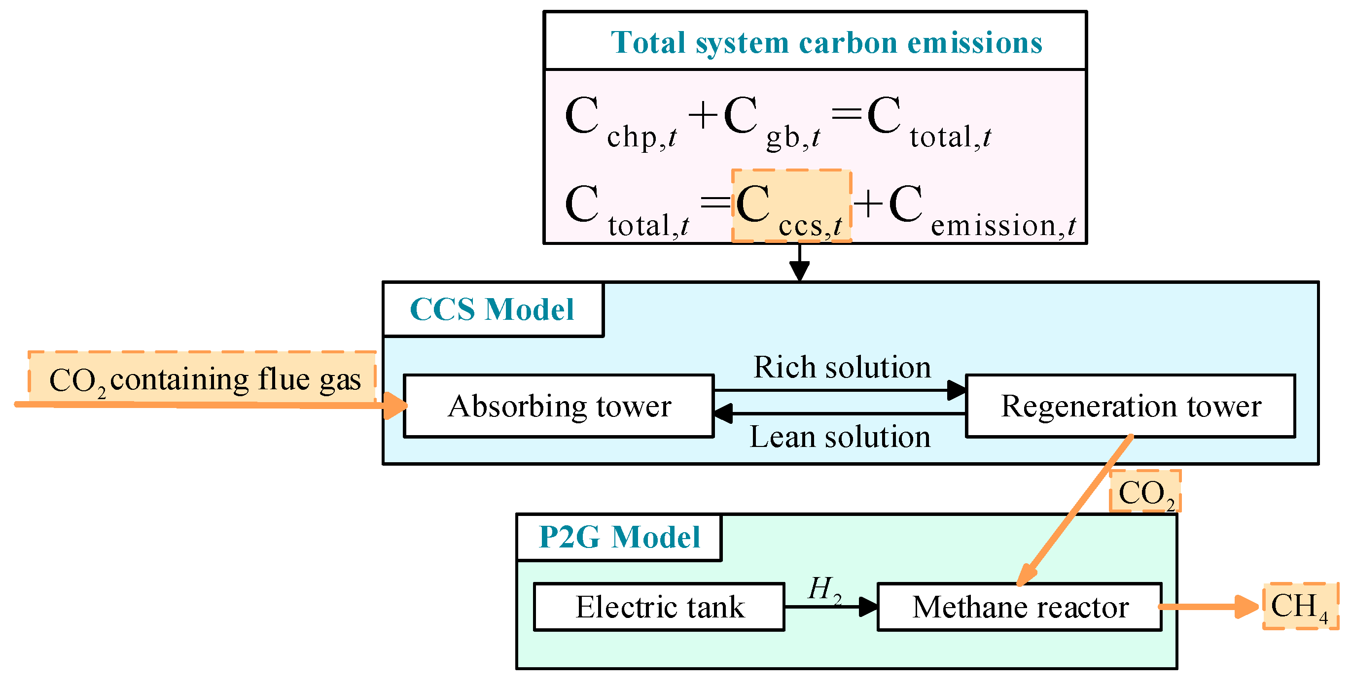
where $E_{\mathrm{wt},t}$ represents the Wind turbines output in time period t; $E_{\mathrm{ccs},t}$ indicates the CCS energy consumption in time period t; $E_{\mathrm{p}2\mathrm{g},t}$ denotes the P2G energy consumption in time period t; and $E_{\mathrm{wte},t}$ signifies the electricity supplied by the WTGs for continued participation in the power system.

2.3. Adjustable Thermoelectric Ratio for CHP

In cogeneration systems, electricity is typically generated by consuming natural gas. In this study, the CHP unit is capable of small-scale oxygen-enriched combustion, enhancing efficiency through the utilization of oxygen stored in the OST, which is generated during the P2G process [33]. Conventional CHP systems are typically categorized into two modes: heat-led and power-led, both of which operate under a fixed heat-to-power ratio. However, this study investigates a CHP system with an adjustable heat-to-power ratio, which dynamically adjusts to daily heating and electricity demands to improve overall operational efficiency. The corresponding operational model is described as follows:

$$\left\{\begin{array}{l}{E}_{\mathrm{chp},e,t}={\eta }_{\mathrm{chp},e}{W}_{g,\mathrm{chp},t}\\ Q_{\mathrm{chp},h,t}={\eta }_{\mathrm{chp},h}{W}_{g,\mathrm{chp},t}\\ W_{g,\mathrm{chp}}^{\min }\le W_{g,\mathrm{chp},t}\le W_{g,\mathrm{chp}}^{\max }\\ \Delta W_{g,\mathrm{chp}}^{\min }\le W_{g,\mathrm{chp},t+1}-W_{g,\mathrm{chp},t}\le \Delta W_{g,\mathrm{chp}}^{\max }\\ {\kappa }_{\mathrm{chp}}^{\min }\le Q_{\mathrm{chp},h,t}/E_{\mathrm{chp},e,t}\le {\kappa }_{\mathrm{chp}}^{\max }\end{array}\right.$$

(6)

where $W_{g,chp,t}$ represents the natural gas power input to the CHP in time period t; $E_{\mathrm{CHP},e}$ and $Q_{\mathrm{CHP},h}$ indicate the electrical and thermal energy output from the CHP in time period t, respectively; ${\eta }_{\mathrm{chp},e}$ and ${\eta }_{\mathrm{chp},h}$ denote the efficiency of conversion of the CHP to electrical and thermal energy, respectively; $W_{g,\mathrm{chp}}^{\max }$ and $W_{g,\mathrm{chp}}^{\min }$ stand for the upper and lower limits of the natural gas power input to the CHP, respectively; $\Delta W_{g,\mathrm{chp}}^{\max }$ and $\Delta W_{g,\mathrm{chp}}^{\min }$ signify the upper and lower limits of the CHP’s creep, respectively; and ${\kappa }_{\mathrm{chp}}^{\max }$ and ${\kappa }_{\mathrm{chp}}^{\min }$ refer to the upper and lower limits of the CHP’s creep, respectively.

2.4. Integrated Energy System Equipment

(1)

Wind turbine

The electrical power output of wind turbines is calculated by:

$$W_{wt}=\left\{\begin{array}{ll}0& (v_{\mathrm{x}}<v_{\mathrm{c}\mathrm{i}})\cup (v_{\mathrm{x}}>v_{\mathrm{c}\mathrm{o}})\\ W_{\mathrm{w}\mathrm{t},\mathrm{r}}(v_{\mathrm{x}}-v_{\mathrm{c}\mathrm{i}})/(v_{\mathrm{r}}-v_{\mathrm{c}\mathrm{i}})& (v_{\mathrm{c}\mathrm{i}}\le v_{\mathrm{x}}\le v_{\mathrm{r}})\\ W_{\mathrm{w}\mathrm{t},\mathrm{r}}& (v_{\mathrm{r}}\le v_{\mathrm{x}}\le v_{\mathrm{c}\mathrm{o}})\end{array}\right.$$

(7)

where $W_{\mathrm{w}\mathrm{t}}$ represents the electrical power of the wind turbine; $v_{\mathrm{x}}$ denotes the actual wind speed at the site; $v_{\mathrm{c}\mathrm{i}}$ and $v_{\mathrm{c}\mathrm{o}}$ signify the minimum and maximum wind speed of the wind turbine, respectively; and $v_{\mathrm{r}}$ indicates the rated wind speed of the wind turbine.

(2)

Solar thermal collector

The thermal power of the solar thermal collectors is calculated by:

$$Q_{\mathrm{st}}=\gamma {\eta }_{\mathrm{st}}S{W}_{\mathrm{st}}$$

(8)

where $Q_{\mathrm{st}}$, $\gamma$, and ${\eta }_{\mathrm{st}}$ represent the collector power, unit conversion coefficient, and efficiency of the collector, respectively; $S$ and $W_{\mathrm{s}\mathrm{t}}$ stand for the collector area and solar radiation intensity, respectively.

(3)

Gas boiler

The GB is activated when the system is insufficiently generating heat and natural gas is needed for heating. The heat produced is calculated by:

$$Q_{\mathrm{gb}}=V_{\mathrm{gb}}{\eta }_{\mathrm{gb}}$$

(9)

where $Q_{\mathrm{gb}}$, $V_{\mathrm{gb}}$, and ${\eta }_{\mathrm{gb}}$ represent the heat generation, gas consumption, and thermal efficiency of the GB equipment, respectively.

(4)

Refrigeration equipment

The system was equipped with two types of refrigeration units: absorption chillers (ACs) and electric chillers (ECs). The AC utilized thermal energy (typically from CHP waste heat) to meet cooling demand, while the EC operated using electrical energy. The allocation of cooling load between these two units depended on the CHP system’s operational mode, particularly the availability of thermal energy.

The corresponding calculation models for the refrigeration units are presented as follows:

$$\left\{\begin{array}{l}{C}_{\mathrm{ac}}=Q_{\mathrm{ac}}{\eta }_{\mathrm{ac}}\\ C_{\mathrm{ec}}=E_{\mathrm{ec}}{\eta }_{\mathrm{ec}}\end{array}\right.$$

(10)

where $C_{\mathrm{ac}}$, $Q_{\mathrm{ac}}$, and ${\eta }_{\mathrm{ac}}$ represent the cooling power, heat energy absorbed, and refrigeration efficiency of an absorption chiller, respectively; $C_{\mathrm{ec}}$, $E_{\mathrm{ec}}$, and ${\eta }_{\mathrm{ec}}$ signify the cooling power, electrical power consumed, and refrigeration efficiency of an electric chiller, respectively.

(5)

Battery

The battery in the system functions to store and release electrical energy. When there is surplus electricity, the battery stores the excess energy; when the electricity supply is insufficient, it discharges the stored energy to meet the demand.

The formula for calculating battery charging and discharging is given as follows:

$$E_t^{ba}=E_{\mathrm{char},t-1}^{ba}{\eta }_{\mathrm{char}}^{ba}-E_{\mathrm{dis},t-1}^{ba}/{\eta }_{\mathrm{dis}}^{ba}+(1-{\eta }_{\mathrm{loss}}^{ba})E_{t-1}^{ba}$$

(11)

where $E_t^{\mathrm{ba}}$, $E_{\mathrm{char}}^{\mathrm{ba}}$, and $E_{\mathrm{dis}}^{\mathrm{ba}}$ denote the state of charge, charging power, and discharging power of the battery in time period t, respectively. ${\eta }_{\mathrm{char}}^{\mathrm{ba}}$, ${\eta }_{\mathrm{dis}}^{\mathrm{ba}}$, and ${\eta }_{\mathrm{loss}}^{\mathrm{ba}}$ represent the charging and discharging efficiency and loss coefficient of the battery, respectively.

(6)

Thermal energy storage tank

The TES system improves thermal energy utilization by capturing and storing excess heat, thereby helping to compensate for thermal energy deficits within the system. The processes of heat absorption and release in TES are calculated as follows:

$$Q_t^{\mathrm{tes}}=Q_{\mathrm{char},t-1}^{\mathrm{tes}}{\eta }_{\mathrm{char}}^{\mathrm{tes}}-Q_{\mathrm{dis},t-1}^{\mathrm{tes}}/{\eta }_{\mathrm{dis}}^{\mathrm{tes}}+(1-{\eta }_{\mathrm{loss}}^{\mathrm{tes}})Q_{t-1}^{\mathrm{tes}}$$

(12)

where $Q_t^{\mathrm{tes}}$, $Q_{\mathrm{char},t}^{\mathrm{tes}}$, and $Q_{\mathrm{dis},t}^{\mathrm{tes}}$ represent the heat storage capacity, heat absorption power, and heat release power of the heat storage tank at time t, respectively; ${\eta }_{\mathrm{char}}^{\mathrm{tes}}$, ${\eta }_{\mathrm{dis}}^{\mathrm{tes}}$, and ${\eta }_{\mathrm{loss}}^{\mathrm{tes}}$ indicate the heat storage efficiency and heat release efficiency of the heat storage tank and the loss coefficient, respectively.

(7)

Oxygen storage tank

The OST recovered the by-products of the electrolysis reaction to avoid the waste of oxygen. The stored oxygen was injected into the cogeneration for oxygen-enriched combustion and power generation to enhance equipment operating efficiency and curtail energy consumption. The OST storage is calculated as follows:

$$V_t^{\mathrm{ost}}=V_{t-1}^{\mathrm{ost}}+{\eta }_{\mathit{char}}^{\mathrm{ost}}{V}_{\mathrm{char},t}^{\mathrm{ost}}-V_{\mathrm{dis},t}^{\mathrm{ost}}/{\eta }_{\mathrm{dis}}^{\mathrm{ost}}$$

(13)

where $V_{t-1}^{\mathrm{ost}}$ represents the volume of oxygen remaining in the oxygen storage tank at time t − 1; $V_{\mathrm{char},t}^{\mathrm{ost}}$ and $V_{\mathrm{dis},t}^{\mathrm{ost}}$ signify the amount of oxygen charged and discharged at time t, respectively; and ${\eta }_{\mathrm{char}}^{\mathrm{ost}}$ and ${\eta }_{\mathrm{dis}}^{\mathrm{ost}}$ denote the efficiency of oxygen charging and discharging in the tank, respectively.

3. Multi-Objective Optimization Method for IES Based on MOBKA-QL

Based on this framework, a multi-objective optimization dispatch model for the IES was developed to minimize economic costs and pollutant emissions while maximizing energy utilization efficiency. The model was addressed using the MOBKA-QL algorithm. Detailed formulations of the model and the corresponding solution methodology are presented below.

3.1. Decision Variables

The CHP unit, as the core equipment in the IES system, operates in an “adjustable heat-to-power ratio” mode and outputs both heat and electricity. In this way, it significantly enhanced the overall energy efficiency of the system and played a crucial role in the performance of other equipment. The gas boiler (GB) was engaged to meet the heat demand when the heat supply was inadequate. Both the AC and the EC were considered components of the heat and electric load, respectively. They fulfilled the cooling load requirements by utilizing energy conversion equipment. The two chillers assisted in diversifying how heat and power were used and met cooling requirements. Meanwhile, the addition of the CCS+P2G system curtailed carbon emissions and consumed wind energy. The resulting methane and oxygen provided combustion energy for the CHP unit. The use of HFCs also diminished multi-stage energy losses. However, the output of these resources cannot be controlled artificially.

The following decision variables were set to coordinate the optimal operating states of the various devices in the IES:

$$\mathrm{X}=[E_{\mathrm{buy}},E_{\mathrm{chp},e},Q_{\mathrm{chp},h},E_{\mathrm{hfc},e},Q_{\mathrm{hfc},h},Q_{\mathrm{ac}},E_{\mathrm{ec}},E_{\mathrm{ccs}},E_{\mathrm{el}},Q_{\mathrm{gb}},E_{\mathrm{ba}},V_{\mathrm{ost}},Q_{\mathrm{tes}}]$$

(14)

Other variables can be obtained through coupling constraints.

3.2. Objective Function

The synergistic benefits of multi-objective scheduling in IES were realized by optimizing equipment configurations and operational strategies and addressing complex constraints, all while ensuring system feasibility. A high-dimensional, multi-objective optimization model was established to minimize economic costs, enhance energy efficiency, and reduce carbon emissions. The proposed model offers a comprehensive framework for IES operation optimization, demonstrating significant improvements in economic performance and environmental impact.

(1)

Economic dispatch: Economic cost minimization

The economic cost of the system encompasses several components: the operational expenses associated with the CCS unit, the costs for operating and maintaining energy conversion and storage equipment, and the expenditure for procuring energy to optimize both electrical and thermal energy use. These components are mathematically formulated as follows:

$$f_1={\displaystyle \sum _{t=1}^{\mathrm{T}}({\mu }_t{E}_{\mathrm{ccs},t}+\varpi M_{\mathrm{ccs},t})}$$

(15)

$$f_2={\displaystyle \sum _{i=1}^{\mathrm{m}}\left(c_i{\displaystyle \sum _t^{\mathrm{T}}{W}_{i,t}}\right)}$$

(16)

$$f_3=f_{\mathrm{buy}}+f_{\mathrm{gas}}$$

(17)

$$\left\{\begin{array}{l}{f}_{\mathrm{buy}}={\displaystyle \sum _{t=1}^{\mathrm{T}}{c}_{\mathrm{buy},t}{E}_{\mathrm{buy},t}}\\ f_{\mathrm{gas}}=c_{\mathrm{gas},t}{\displaystyle \sum _{t=1}^{\mathrm{T}}(V_{\mathrm{chp},t}+V_{\mathrm{gb},t})}\end{array}\right.$$

(18)

$$\min F_1=f_1+f_2+f_3$$

(19)

where ${\mu }_t$ represents the operating coefficient of the carbon capture system; $\varpi$ denotes the cost coefficient of carbon capture and storage of ${\mathrm{C}\mathrm{O}}_2$; $M_{\mathrm{ccs},t}$ signifies the amount of carbon capture and storage of ${\mathrm{C}\mathrm{O}}_2$ in time period t; $c_{\mathrm{buy},t}$ stands for the price of electricity in time period t; $c_i$ refers to the coefficient of operation of device i in time period t; $m$ is the number of the devices; $W_{i,t}$ symbolizes the output of device i in time period t; $f_{\mathrm{buy}}$ and $f_{\mathrm{gas}}$ embody the cost of purchasing electricity and natural gas; n $c_{\mathrm{gas},t}$ exemplifies the price of natural gas in time period t.

(2)

Energy dispatch: Energy efficiency maximizing

The IES reinforced energy utilization efficiency by incorporating various energy sources. In this study, both the quantity and quality of energy were considered to maximize energy efficiency, which served as the second optimization objective [29]. Energy use efficiency effectively evaluated the high-quality consumption of energy and ensured the optimal use of different energy types. The specific expressions for this are:

$$\begin{array}{l}\max F_2={\displaystyle \sum _{\mathrm{t}=1}^{\mathrm{T}}{\left(E_{\mathrm{Eload},t}+E_{\mathrm{char},t}^{\mathrm{ba}}+{\omega }_1(Q_{\mathrm{Qload},t}+Q_{\mathrm{char},t}^{\mathrm{tes}})+{\omega }_2{C}_{\mathrm{Cload},t}+E_{\mathrm{ccs},t}+E_{\mathrm{p}2\mathrm{g},t}\right)}_{\max }}/\\ {\displaystyle \sum _{t=1}^{\mathrm{T}}{\left(E_{\mathrm{buy},t}+E_{\mathrm{wt},t}+E_{\mathrm{dis},t}^{\mathrm{ba}}+{\omega }_1(Q_{\mathrm{dis},t}^{\mathrm{tes}}+Q_{\mathrm{hfc},h,t}+Q_{\mathrm{st},t})+E_{\mathrm{hfc},e,t}+L_{{\mathrm{CH}}_4}(V_{\mathrm{gas},t}+V_{\mathrm{mr},t})\right)}_{\min }}\end{array}$$

(20)

where the numerator and the denominator represent the required load and energy supply of the integrated energy system, respectively; $E_{\mathrm{Eload},t}$, $Q_{\mathrm{Qload},t}$, and $C_{\mathrm{Cload},t}$ indicate the electrical, thermal, and cooling loads in time period t, respectively; $E_{\mathrm{char},t}^{\mathrm{ba}}$ denotes the electrical energy stored by the battery in time period t; $Q_{\mathrm{char},t}^{\mathrm{tes}}$ signifies the thermal energy stored in the thermal energy storage tank in time period t; $E_{\mathrm{dis},t}^{\mathrm{ba}}$ describes the electrical energy released from the battery in time period t; $Q_{\mathrm{dis},t}^{\mathrm{tes}}$ expresses the thermal energy released by the thermal energy storage tank in time period t; $V_{\mathrm{gas},t}$ indicates natural gas purchased by the system; $V_{\mathrm{mr},t}$ reflects the natural gas supplied by MR in the P2G process; ${\omega }_1$ specifies the conversion coefficient between thermal and electrical energy sources; and ${\omega }_2$ denotes the conversion coefficient between cold and electrical energy sources.

(3)

Low-carbon dispatch: Carbon dioxide emissions minimizing

The total carbon emissions of the system were diminished to reduce environmental pollution, highlighting the environmental advantages of the IES. The objective function for the system’s pollutant gas emissions is defined as:

$$\min F_3={\displaystyle \sum _{t=1}^{\mathrm{T}}{E}_{\mathrm{chp},t}{\displaystyle \sum _{j=1}^{\mathrm{n}}{c}_j{m}_{\mathrm{chp},j}}+Q_{\mathrm{gb},t}{\displaystyle \sum _{j=1}^{\mathrm{n}}{c}_j{m}_{\mathrm{gb},j}+E_{\mathrm{buy},t}{\displaystyle \sum _{j=1}^{\mathrm{n}}{m}_{\mathrm{buy},j}}-M_{\mathrm{ccs},t}}}$$

(21)

where $m_{\mathrm{chp},j}$, $m_{\mathrm{gb},j}$, and $m_{\mathrm{buy},j}$ represent the pollutant emission factors for CHP, GB, and electricity purchased from the grid, respectively; n denotes the amount of pollutant gases, mainly including ${\mathrm{CO}}_2$, ${\mathrm{SO}}_2$, and ${\mathrm{NO}}_{\mathrm{x}}$; and ${\mathrm{M}}_{\mathrm{ccs},t}$ indicates the amount of ${\mathrm{CO}}_2$ captured by the carbon capture and storage system.

3.3. Constraints

(1)

Output constraints for devices in the system

$$\left\{\begin{array}{l}0\le E_{\mathrm{wt},t}\le E_{\mathrm{wt}}^{\max }\\ 0\le Q_{\mathrm{st},t}\le Q_{\mathrm{st}}^{\max }\\ 0\le E_{\mathrm{ccs},t}\le E_{\mathrm{ccs}}^{\max }\\ Q_{\mathrm{gb},t}={\eta }_{\mathrm{gb}}{W}_{gas,\mathrm{gb}}\\ W_{gas,\mathrm{gb}}^{\min }\le W_{gas,\mathrm{gb}}\le W_{gas,\mathrm{gb}}^{\max }\\ \Delta W_{gas,\mathrm{gb}}^{\min }\le W_{gas,\mathrm{gb},t+1}-W_{gas,\mathrm{gb},t}\le \Delta W_{gas,\mathrm{gb}}^{\max }\end{array}\right.$$

(22)

where $E_{\mathrm{wt}}^{\max }$ signifies the upper limit of wind power output; $Q_{\mathrm{st}}^{\max }$ refers to the upper power limit of solar collectors to capture thermal energy; $E_{\mathrm{ccs}}^{\max }$ reflects the upper limit of CCS; $W_{gas,\mathrm{gb}}^{\max }$ and $W_{gas,\mathrm{gb}}^{\min }$ describe the upper and lower limits of input power to GB, respectively; and $\mathsf{\Delta }{W}_{gas,\mathrm{gb}}^{\max }$ and $\mathsf{\Delta }{W}_{gas,\mathrm{gb}}^{\min }$ symbolize the upper and lower limits of climb of GB, respectively.

(2)

Electricity purchase constraints

On-system purchases of power from the main grid are restricted.

$$0\le E_{\mathrm{buy},t}\le E_{\mathrm{buy}}^{\max }$$

(23)

where ${\mathrm{E}}_{\mathrm{b}\mathrm{u}\mathrm{y}}^{\mathrm{m}\mathrm{a}\mathrm{x}}$ represents the maximum power of purchased electricity in time period t.

(3)

Energy storage device constraints

This paper has the same operation mechanism for the three types of energy storage devices: electrical, thermal, and oxygen. Thus, the energy storage devices were modeled in a standardized manner [34], expressed as:

$$\left\{\begin{array}{l}0\le W_{\mathrm{es},n,t}^{\mathrm{char}}\le B_{\mathrm{es},n,t}^{\mathrm{char}}{W}_{\mathrm{es},n}^{\max }\\ 0\le W_{\mathrm{es},n,t}^{\mathrm{dis}}\le B_{\mathrm{es},n,t}^{\mathrm{dis}}{W}_{\mathrm{es},n}^{\max }\\ W_{\mathrm{es},n,t}=W_{\mathrm{es},n,t}^{\mathrm{char}}/{\eta }_{\mathrm{es},n}^{\mathrm{char}}-W_{\mathrm{es},n,t}^{\mathrm{dis}}/{\eta }_{\mathrm{es},n}^{\mathrm{dis}}\\ S_{n,t}=S_{n,t-1}+W_{\mathrm{es},n,t}/W_{\mathrm{es},n}^{\mathrm{cap}}\\ S_{n,1}{=\mathrm{S}}_{n,\mathrm{T}}\\ B_{\mathrm{es},n,t}^{\mathrm{char}}+B_{\mathrm{es},n,t}^{\mathrm{dis}}=1\\ S_n^{\min }\le S_{n,t}\le S_n^{\max }\end{array}\right.$$

(24)

where $W_{\mathrm{es},n}^{\mathrm{char}}$ and $W_{\mathrm{es},n}^{\mathrm{dis}}$ represent the charging and discharging power of the nth type of energy storage device in time period t, respectively; $W_{\mathrm{es},n}^{\max }$ denotes the maximum power of the nth type of energy storage device in a single charging and discharging; $B_{\mathrm{es},n,t}^{\mathrm{char}}$ and $B_{\mathrm{es},n,t}^{\mathrm{dis}}$ are binary variables, reflecting the charging and discharging state parameters of the nth type of energy storage device in time period t; $B_{\mathrm{es},n,t}^{\mathrm{char}}=1$ and $B_{\mathrm{es},n,t}^{\mathrm{dis}}=0$ indicate that it is in the charging state; $B_{\mathrm{es},n,t}^{\mathrm{char}}=0$ and $B_{\mathrm{es},n,t}^{\mathrm{dis}}=1$ suggest that it is in the discharging state; $W_{\mathrm{es},n,t}$ describes the final output power of the nth type of energy storage device in time period t; ${\eta }_{\mathrm{ES},n}^{\mathrm{char}}$ and ${\eta }_{\mathrm{ES},n}^{\mathrm{dis}}$ refer to the charging and discharging power of the nth type of energy storage device, respectively; $S_{n,t}$ stands for the capacity of the nth type of energy storage device in time period t; $W_{\mathrm{es},n}^{\mathrm{cap}}$ embodies the rated capacity of the nth type of energy storage device; and $S_n^{\max }$ and $S_n^{\min }$ signify the upper and lower limits of the capacity of the nth type of energy storage device, respectively.

(4)

The constraints of CCS, P2G, and CHP equipment are expressed in Equations (1)–(3) and (6).

(5)

Cold power balance constraints

$$\left\{\begin{array}{l}{Q}_{\mathrm{ac}}^{\min }\le Q_{\mathrm{ac},t}\le Q_{\mathrm{ac}}^{\max }\\ E_{\mathrm{ec}}^{\min }\le E_{\mathrm{ec},t}\le E_{\mathrm{ec}}^{\max }\\ Q_{\mathrm{ac},t}+E_{\mathrm{ec},t}=C_{\mathrm{Cload},t}\end{array}\right.$$

(25)

where $Q_{\mathrm{ac},t}$ represents the power required by the absorption chiller in time period t; $Q_{\mathrm{ac}}^{\min }$ and $Q_{\mathrm{ac}}^{\max }$ signify the upper and lower limits of the power of the absorption chiller in time period t, respectively; $E_{\mathrm{ec},t}$ indicates the power required by the electric chiller in time period t; $E_{\mathrm{ec}}^{\min }$ and $E_{\mathrm{ec}}^{\max }$ denote the upper and lower limits of the power of the electric chiller in time period t, respectively; and $C_{\mathrm{Cload},t}$ embodies the cooling load demand in time period t.

(6)

Electric power balance constraints

$$E_{\mathrm{chp},t}+E_{\mathrm{wt},t}+E_{\mathrm{hfc},t}+E_{\mathrm{char},t}^{\mathrm{ba}}+E_{\mathrm{buy},t}=E_{\mathrm{ec},t}+E_{\mathrm{p}2\mathrm{g},t}+E_{\mathrm{ccs},t}+E_{\mathrm{Eload},t}+E_{\mathrm{dis},t}^{\mathrm{ba}}$$

(26)

(7)

Thermal power balance constraints

$$Q_{\mathrm{st},t}+Q_{\mathrm{chp},t}+Q_{\mathrm{gb},t}+Q_{\mathrm{hfc},t}+Q_{\mathrm{tes},\mathrm{char},t}=Q_{\mathrm{ac},t}+Q_{\mathrm{Qload},t}+Q_{\mathrm{tes},\mathrm{dis},t}$$

(27)

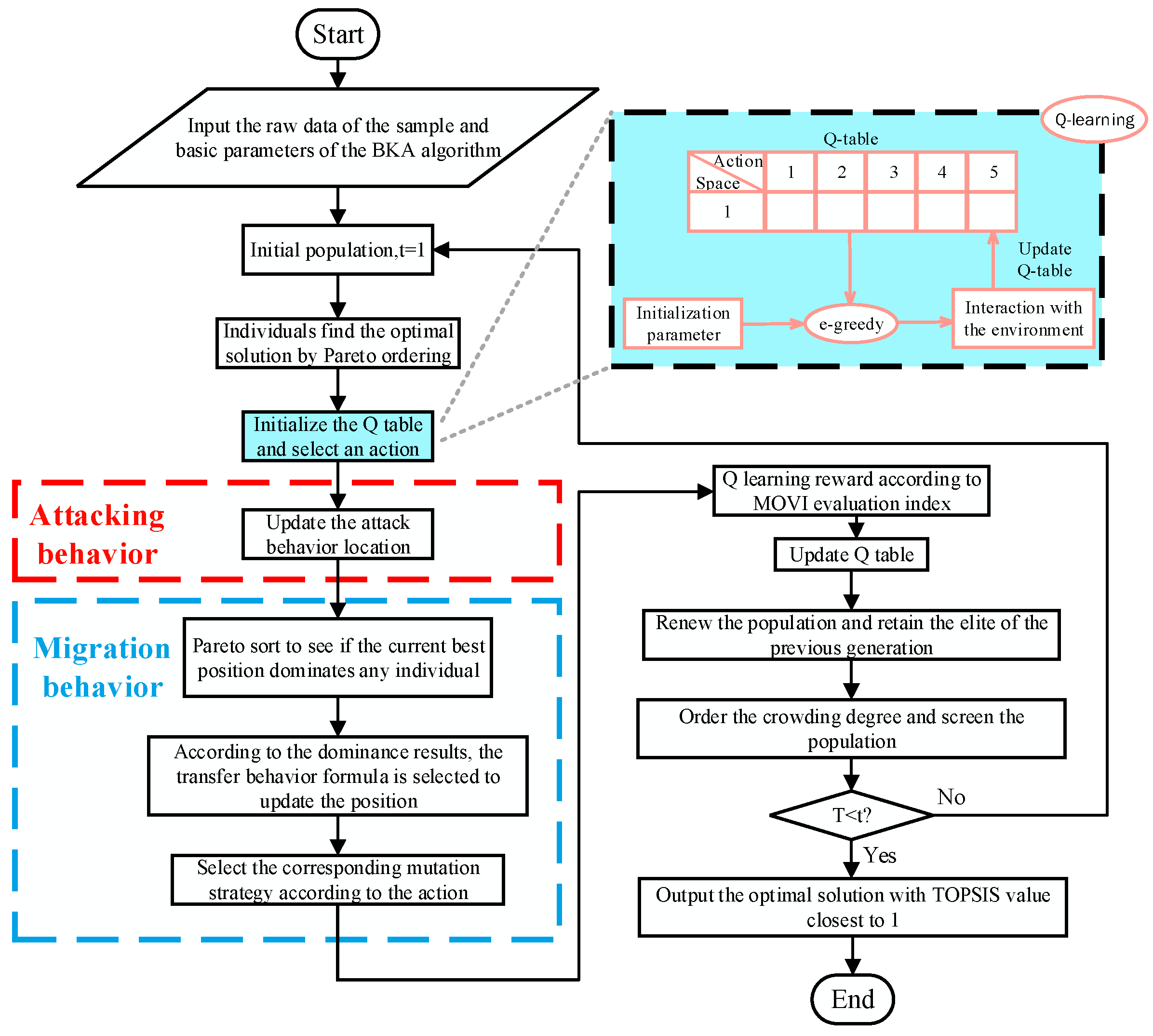
3.4. Improved Multi-Objective Black-Winged Kite Algorithm with Adaptive Mutation Based on Q-Learning

The Black-winged Kite Algorithm (BKA), as a novel metaheuristic approach, demonstrates efficient optimization capabilities for constrained problems while exhibiting strong robustness and superior convergence performance. To address the challenges of multi-objective IES optimization—including obtaining well-distributed Pareto solutions and avoiding local optima—this study enhances the original BKA by integrating multi-objective optimization with Pareto ranking, Q-learning for adaptive parameter tuning, and multiple mutation strategies to maintain population diversity. The resulting MOBKA-QL algorithm effectively solves the proposed model, achieving balanced optimization across competing objectives.

3.4.1. BKA

The BKA was developed by simulating the predatory and migratory behaviors of black-winged kites in nature. It adopts a global search strategy inspired by whole-map migration patterns. The mechanism is defined as follows:

(1)

Initialization phase

$$y^{i,j}=B{K}_{dl}+rand(B{K}_{ul}-B{K}_{dl})$$

(28)

(2)

Attacking behavior

$$y_{t+1}^{i,j}=\left\{\begin{array}{ll}{y}_t^{i,j}+n(1+\sin (r))\times y_t^{i,j}& p<r\\ y_t^{i,j}+n(2r-1)\times y_t^{i,j}& \mathrm{else}\end{array}\right.$$

(29)

$$n=0.05\times {\mathrm{e}}^{-2\times {({\displaystyle \frac{t}{\mathrm{T}}})}^2}$$

(30)

(3)

Migration behavior

$$y_{t+1}^{i,j}=\left\{\begin{array}{ll}{y}_t^{i,j}+c(0,1)\times (y_t^{i,j}-L_t^j)& F_i<F_{ri}\\ y_t^{i,j}+c(0,1)\times (L_t^j-m\times y_t^{i,j})& \mathrm{else}\end{array}\right.$$

(31)

$$m=2\times \sin (r+\pi /2)$$

(32)

$$f(x,\delta ,\mu )=\delta /\pi ({\delta }^2+{(x-\mu )}^2)\hspace{1em}-\infty <x<\infty$$

(33)

where $B{K}_{dl}$ and $B{K}_{ul}$ represent the next and previous sessions of the ith black-winged kite in the jth dimension, respectively; $y_t^{i,j}$ and $y_{t+1}^{i,j}$ denote the position of the ith black-winged kite in the jth dimension in the tth and (t + 1)th iteration, respectively; r indicates a random number with a value ranging from 0 to 1; p signifies the parameter controlling the behavior of different attacks; T refers to the total number of iterations; t stands for the number of iterations that have been completed so far; $L_t^j$ describes the leading scorer of the jth dimensional black-winged kite in the tth iteration so far; $F_i$ expresses the jth dimensional current position obtained by any black-winged kite in the tth iteration; $F_{ri}$ embodies the fitness value of any black-winged kite in the jth dimensional random position in the tth iteration; and C(0, 1) symbolizes the Cauchy mutation defined as in Equation (33).

The traditional black-winged kite algorithm has shortcomings such as a lack of global optimal exploration ability, parameter sensitivity, and slow convergence speed, which were addressed in this paper.

3.4.2. Selection of Multiple Mutation Strategies for MOBKA-QL

The original BKA tends to excessively focus on certain regions of the solution space while neglecting others, leading to premature convergence near local optima and hindering its ability to locate the global optimum. In IES, the complexity increases with the number of devices and operational constraints, resulting in an extensive range of possible scheduling plans. Therefore, it is essential for the optimization algorithm to escape local optima to explore more feasible and diverse operating strategies. Mutation strategies address this issue by enhancing population diversity and expanding the search space. By incorporating adaptive mutation strategies, our research group has significantly improved BKA’s performance in solving complex optimization problems.

This paper integrates thirteen commonly used mutation strategies into the BKA algorithm, as summarized in

Table 1. Summary of the 13 variant strategy formulas.

Variation Strategy	Variation Formula
Gaussian variation	$x\sim N\left(\mu ,{\sigma }^2\right),mx=x$
Gaussian elite variation	$r\sim N\left(\mu ,{\sigma }^2\right),mx=r.\ast x$
Cauchy variation	$mx=x_{\mathrm{best}}+\left({\displaystyle \frac{\sigma }{\pi ({(x-\mu )}^2+{\sigma }^2}}\right).\ast x_{\mathrm{best}}$
Inverse cumulative distribution function	$mx=\tan \left(\pi \left(r_p-{\displaystyle \frac{1}{2}}\right)\right)$
t-distribution variation	$mx=x_{\mathrm{best}}+x_{\mathrm{best}}.\ast t_{\mathrm{rnd}}(t)$
Adaptive t-distribution variation	$mx=x_{\mathrm{best}}+x_{\mathrm{best}}.\ast t_{\mathrm{rnd}}(\exp {\left({\displaystyle \frac{t}{\mathrm{T}}}\right)}^2)$
Normal cloud variation	$E_n=\exp ({\displaystyle \frac{t}{\mathrm{T}}}),ra=N(x_{best},\left|E_n\right|),mx=\exp \left(-{\displaystyle \frac{{\left(ra-x_{\mathrm{best}}\right)}^2}{2E_n^2}}\right)$
Periodic variation	$mx=x.\ast \left(1.5-rand\left(1,dim\right)\right)$
Elite differential variation 1	$mx=x_{\mathrm{best}}+rand.\ast (x_{r1}-x_{r2})$
Random elite differential variation	$mx=x+rand.\ast (x_{\mathrm{best}}-x)+rand.\ast (x_{\mathrm{r}1}-x_{r2})$
Random difference variation	$mx=x_{r1}+rand.\ast (x_{r2}-x_{r3})+rand.\ast (x_{\mathrm{r}4}-x_{r5})$
Elite differential variation 2	$mx=x_{\mathrm{best}}+rand.\ast (x_{r1}-x_{r2})+rand.\ast (x_{\mathrm{r}3}-x_{r4})$
Heterogeneous variation	$p=1-{\displaystyle \frac{t}{T}},mx=\left\{\begin{array}{ll}x+(ul-x).\ast (1-ran{d}^{p^b})& if\hspace{0.17em}F=0\\ x-(x-dl).\ast (1-ran{d}^{p^b})& if\hspace{0.17em}F=1\end{array}\right.$

. The mutation operations generate updated individuals (denoted as mx), which represent modified versions of the original solutions x [24,25,35,36,37,38,39]. Through multi-iteration performance evaluation, five superior mutation strategies were selected, with their comparative effectiveness illustrated in Figure 4.

As shown in Figure 4, the five most effective mutation strategies were identified as periodic variation, random-elite differential variation, random differential variation, elite differential variation, and heterogeneous variation. Therefore, all five mutation strategies were incorporated into the migration behavior update formula (Equation (31)).

3.4.3. Implementation of Adaptive Mutation Strategies Based on Q-Learning

In this study, Q-learning serves as a control mechanism to dynamically select optimal mutation strategies during each iteration, based on real-time system states and evaluation results. The algorithm updates the Q-table through a reward mechanism that evaluates Multi-Objective Variation Index (MOVI) differences between consecutive iterations, thereby adaptively adjusting strategy selection probabilities. This approach enables optimal action selection at each iteration stage, significantly enhancing the algorithm’s adaptability and search efficiency.

MOVI quantitatively measures solution set diversity and evaluates mutation strategy effectiveness. When MOVI increases, it provides positive feedback indicating improved solution set distribution quality. This mechanism guides the algorithm toward more diverse exploration patterns, effectively reducing local optima entrapment risks while promoting stable convergence behavior.

In this mechanism, the algorithm’s actions interact with the environment: each selected action modifies the system state, while the environment provides feedback through a reward function that quantifies the action’s effectiveness [40]. This feedback subsequently guides future decision-making processes. This design achieves an effective balance between reinforcing successful mutation strategies and preserving solution diversity, eliminating the need for additional performance indicators. Consequently, it establishes a dynamic yet stable search scheduling mechanism. The Q-table update formula is formally defined as:

$$Q(s,a)\to Q(s,a)+\alpha [r+\gamma {\max }_{a^{\prime }}Q(s^{\prime },a^{\prime })-Q(s,a)]$$

(34)

where $Q(s,a)$ represents the Q-value of taking an action in states; r denotes the reward obtained after the execution of that action; $\gamma$ signifies the decay coefficient; and $Q(s^{\prime },a^{\prime })$ embodies the Q-value of taking an action in the next state.

In this paper, Q-learning was employed to achieve adaptive mutation of the update formula, with the following parameters requiring definition:

(1)

State

The one-step Q-learning method implemented in this study utilizes only immediate state–action pairs for Q-value updates, fulfilling dynamic search requirements during iterations. This computationally efficient approach ensures fast environmental adaptation and excellent real-time decision-making performance.

(2)

Action

Five common variant strategies with good improvements to MOBKA-QL were selected following the above discussion. Hence, these strategies were chosen to form action sets to dynamically adjust the search capability and position at different stages.

Action 1: Mutation strategy selects periodic variation.

Action 2: Variation strategy selects random elite differential variation.

Action 3: Mutation strategy selects random difference variation.

Action 4: Mutation strategy selects elite differential variation.

Action 5: Variation strategy selects heterogeneous variation.

(3)

Award

In this paper, the Multi-Objective Variance Indicator (MOVI) is used to evaluate optimization performance by comparing MOVI values between consecutive iterations. A negative reward (−1) is assigned when the population shows poor performance and a positive reward (+2) is given otherwise. To reinforce effective exploration while avoiding premature elimination of strategies, an asymmetric reward mechanism is adopted. This design balances learning efficiency and policy stability by encouraging the retention of well-performing mutation strategies while maintaining exploration capability.

To verify the effectiveness of the reward settings, a sensitivity analysis was conducted using three schemes: (1) symmetric (+1/−1), (2) over-penalized (+1/−5), and (3) the proposed asymmetric positive scheme (+2/−1). As shown in

Table 2. Comparative effect experiment of reward mechanism design.

Reward Mechanism	Average MOVI Improvement	Convergence Times	Number of Non-Dominated Solutions
Symmetrical (+1/−1)	0.083	78	35
Excessive punishment (+1/−5)	0.071	92	28
Asymmetric (+2/−1)	0.096	51	40

, the proposed reward configuration achieves better performance in MOVI improvement, convergence speed, and the number of non-dominated solutions, demonstrating higher learning efficiency and multi-objective optimization capability.

The final reward scheme is therefore set as follows:

$$r_t=\left\{\begin{array}{ll}+2,& if\hspace{0.33em}MOV{I}_t>MOV{I}_{t-1}\\ -1,& \hfill \mathrm{else}\hfill \end{array}\right.$$

(35)

where $r_t$ and $MOV{I}_t$ represent the reward and metric values of state t, respectively.

(4)

Epsilon calculation

Dynamic computation of epsilon, which was used to control the trade-off between exploration and utilization in the $\epsilon -greedy$ strategy, was performed by the following equation. By adjusting epsilon dynamically, the algorithm adopts different strategies at different learning stages, thereby enhancing learning efficiency and effectiveness. In the initial stage, epsilon is set higher to encourage extensive exploration and comprehensive experience acquisition; in later stages, epsilon is gradually reduced to emphasize the exploitation of the learned knowledge and improve learning efficiency. This smooth transition balances exploration and exploitation, ultimately leading to improved overall learning performance.

$$epsilon=Wa-(Wa-Wb)\ast (t/\mathrm{T})$$

(36)

where Wa represents the initial high exploration weight and Wb indicates the final low exploration weight.

3.4.4. Multi-Objective Optimization of the MOBKA-QL Algorithm

The BKA was originally designed for single-objective optimization, using fitness values to evaluate solutions and guide search behavior. To address the simultaneous optimization of economy, carbon emissions, and energy efficiency in IES, this study extends the original BKA framework to a multi-objective version called MOBKA-QL. This new algorithm combines Q-learning with a Pareto dominance mechanism, enabling dynamic updates of the solution set and effective simultaneous optimization of multiple objectives.

In MOBKA-QL, the evaluation of individual solutions no longer depends on a single fitness value but is instead based on Pareto ranking, which improves the balance of the solution set. In particular, considering that the original BKA used fitness-based comparisons to determine migration behavior, this study proposed an improved strategy: update rules are selected based on the dominance relationship between the current individual $y_t^{i,j}$ and the historical Pareto-optimal $P^{*}$ archive. As a convergence-oriented behavior, migration enhances local search ability and accelerates convergence to optimal solutions.

To further improve adaptability in complex multi-objective environments, a Q-learning-based dynamic mutation strategy was embedded into the migration process. This mechanism allows the algorithm to adjust mutation strategies based on feedback from the search environment, thus achieving a better balance between global exploration and local exploitation while enhancing solution diversity and convergence stability.

The specific logic of the improved migration behavior is as follows:

$$y_{t+1}^{i,j}=\left\{\begin{array}{ll}{y}_t^{i,j}+c(0,1)\times (y_t^{i,j}-L_t^j)& \mathrm{if}\hspace{0.17em}\exists \hspace{0.17em}{x}^{*}\in P^{*}:x^{*}\prec y_t^i\\ y_t^{i,j}+c(0,1)\times (L_t^j-m\times y_t^{i,j})& \mathrm{else}\end{array}\right.$$

(37)

where $x^{*}\prec y_t^i$ represents that the historical Pareto archive $x^{*}$ dominates the current individual $y_t^i$; $L_t^j$ indicates the optimal solution in the j-th objective within the historical Pareto archive.

3.4.5. Optimization Result Selection for the MOBKA-QL Algorithm

In this paper, the optimal solutions from both the previous and current generations were combined and sorted by Pareto dominance to preserve optimal solutions across iterations. As the optimization progresses and the solution sets merge, the Pareto front gradually grows. To maintain an even distribution of individuals, the crowding distance was used to measure population density [41]. The size of the solution set was controlled by imposing an upper limit on the crowding distance. If the number of individuals at the optimal dominance level did not exceed this limit, all were included in the new population. Otherwise, individuals were selected based on their crowding distance in descending order until the limit was reached, and any remaining individuals were discarded.

The formula for calculating the multi-objective congestion distance is:

$$n_d=n_{di}+(F_m(i+1)-F_m(i-1))/(F_{\max }-F_{\min })$$

(38)

where $F_m(i+1)$ and $F_m(i-1)$ indicate the values of the objective functions corresponding to the two neighboring individuals before and after the black-winged kite individual i, respectively; $n_{di}$ denotes the congestion distance for a particular objective function; and $n_d$ signifies the total congestion distance for multiple objective functions.

The solution set was selected from the above solution set with the TOPSIS value closest to 1 after the Pareto and crowding degree calculations as the optimal solution. At this point, the solution is the optimal scheduling solution.

3.4.6. MOBKA-QL Algorithm Steps

Figure 5 illustrates the detailed solution process of the MOBKA-QL.

3.4.7. Benchmark Testing and Result Analysis of the MOBKA-QL Algorithm

To verify the effectiveness of the improved MOBKA-QL algorithm in multi-objective optimization, four representative benchmark algorithms—MOSSA, MOPSO, MODE, and MOGOOSE—were selected for comparison. Performance evaluations were conducted on two standard test functions, Viennet2 and DTLZ2. The experimental results are presented in Figure 6, which illustrates the Pareto front distributions obtained by each algorithm under the respective test functions.

Figure 6a shows the results for the Viennet2 function. Due to its pronounced curvature and turning regions on the Pareto front, this function poses challenges to both global exploration and local exploitation capabilities. As can be seen from the figure, the solution set obtained by MOBKA-QL is overall well-distributed, with clear boundaries and moderate density. It not only covers a majority of the Pareto front but also effectively fills the sparse regions with significant curvature changes, demonstrating strong resolution and adaptability. Figure 6b,c depict the Pareto front distributions of the DTLZ2 test function, where Figure 6b provides a side view and Figure 6c a front view. From Figure 6b, it can be observed that the solution set of MOBKA-QL closely adheres to the theoretical Pareto front surface, forming a regular and coherent shape, indicating good convergence. In Figure 6c, the MOBKA-QL solutions exhibit higher density and more uniform distribution, achieving comprehensive coverage of the front surface in the objective space. In contrast, the other algorithms display varying degrees of deviation or non-uniformity in both views, with phenomena such as solution drift or sparsity, suggesting that MOBKA-QL offers superior stability and global coverage capability.

4. Simulation and Analysis

A series of experimental analyses were designed and conducted with load and energy forecast data for typical seasons in a specific region to validate the effectiveness of the proposed IES model and MOBKA-QL algorithm. The comparative analysis of the experimental results further revealed the feasibility and advantages of the proposed method in practical applications. The specific methods of this study are exhibited in Figure 7.

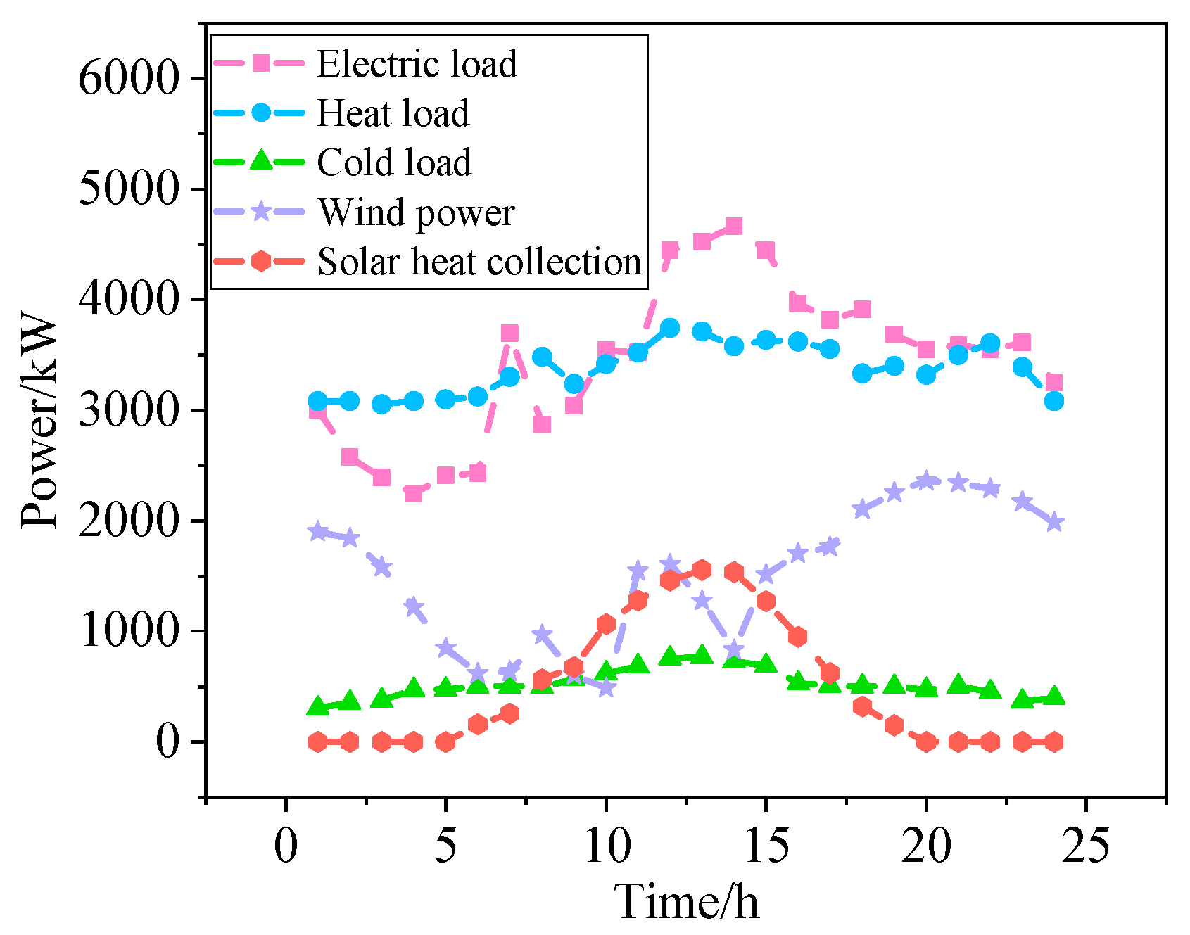
4.1. Original Data

The experiments in this section were based on typical seasonal forecast data for cooling, heating, electric load, and renewable energy in specific regions of China. The scheduling period spanned 24 h, with each hour representing one time step. The forecasts of renewable energy production, electricity, heating, and cooling loads are depicted in Figure 8. The parameters of each device in IES are provided in

Table 3. IES system device parameters setting.

Parameters	Values	Parameters	Values	Parameters	Values
${\eta }_{\mathrm{e}\mathrm{l}}$	0.85	${\eta }_{\mathrm{c}\mathrm{h}\mathrm{a}\mathrm{r}}^{\mathrm{t}\mathrm{h}\mathrm{s}}$	0.95	${\eta }_{\mathrm{p}2\mathrm{g}}$	0.56
${\eta }_{m\mathrm{r}}$	0.7	${\eta }_{\mathrm{d}\mathrm{i}\mathrm{s}}^{\mathrm{t}\mathrm{h}\mathrm{s}}$	0.95	${\eta }_{\mathrm{g}\mathrm{b}}$	0.85
${\eta }_{\mathrm{hfc},e}$	0.785	${\eta }_{\mathrm{l}\mathrm{o}\mathrm{s}\mathrm{s}}^{\mathrm{t}\mathrm{h}\mathrm{s}}$	0.01	${\eta }_{\mathrm{a}\mathrm{c}}$	0.93
${\eta }_{\mathrm{hfc},\mathrm{h}}$	0.613	${\eta }_{\mathrm{c}\mathrm{h}\mathrm{a}\mathrm{r}}^{\mathrm{o}\mathrm{s}\mathrm{t}}$	0.95	${\eta }_{\mathrm{e}\mathrm{c}}$	0.6
$m_{{\mathrm{chp},\mathrm{CO}}_2}$	0.724 t/kWh	${\eta }_{\mathrm{d}\mathrm{i}\mathrm{s}}^{\mathrm{o}\mathrm{s}\mathrm{t}}$	0.95	$E_{\mathrm{hfc}}^{\max }$	800 kWh
$m_{{\mathrm{chp},\mathrm{SO}}_2}$	0.00328 t/kWh	$\mathrm{\varpi }$	35	$E_{\mathrm{el}}^{\max }$	1000 kWh
$m_{{\mathrm{chp},\mathrm{NO}}_{\mathrm{x}}}$	0.00376 t/kWh	${\omega }_1$	0.5	$E_{\mathrm{mr}}^{\max }$	800 kWh
$m_{{\mathrm{buy},\mathrm{CO}}_2}$	0.55 t/kWh	${\omega }_2$	0.25	$E_{\mathrm{buy}}^{\max }$	3000 kWh
${\eta }_{\mathrm{c}\mathrm{h}\mathrm{a}\mathrm{r}}^{\mathrm{b}\mathrm{a}}$	0.95	${\kappa }_{\mathrm{c}\mathrm{h}\mathrm{p}}^{\max }$	2	$m_{{\mathrm{gb},\mathrm{CO}}_2}$	0.392 t/kWh
${\eta }_{\mathrm{d}\mathrm{i}\mathrm{s}}^{\mathrm{b}\mathrm{a}}$	0.95	${\kappa }_{\mathrm{c}\mathrm{h}\mathrm{p}}^{\min }$	0.5	$m_{{\mathrm{gb},\mathrm{SO}}_2}$	0.0016 t/kWh
${\eta }_{\mathrm{l}\mathrm{o}\mathrm{s}\mathrm{s}}^{\mathrm{b}\mathrm{a}}$	0.1	${\rho }_{{\mathrm{H}}_2}$	4 m3	$m_{{\mathrm{gb},\mathrm{NO}}_{\mathrm{x}}}$	0.00197 t/kWh
$\mathrm{\beta }$	0.33 kWh/h	$L_{{\mathrm{CH}}_4}$	11 kWh	$c_{\mathrm{ec}}$	0.01 ¥/kWh
${\rho }_{\mathrm{C}{\mathrm{O}}_2}$	1 m3	$E_{\mathrm{ccs}}^{\max }$	500 kW	$c_{\mathrm{el}}$	0.096 ¥/kWh
$E_{\mathrm{wt}}^{\max }$	3000 kWh	$Q_{\mathrm{gb}}^{\max }$	1500 kW	${\mathrm{c}}_{\mathrm{mr}}$	0.122 ¥/kWh
$Q_{\mathrm{st}}^{\max }$	2000 kWh	$c_{\mathrm{chp}}$	0.13 ¥/kWh	$c_{\mathrm{ost}}$	0.065 ¥/kWh
$E_{\mathrm{ec}}^{\max }$	800 kWh	$c_{\mathrm{hfc}}$	0.0835 ¥/kWh	$c_{\mathrm{ac}}$	0.024 ¥/kWh
$Q_{\mathrm{ac}}^{\max }$	800 kWh	$c_{\mathrm{gb}}$	0.028 ¥/kWh	$c_{\mathrm{tes}}$	0.01 ¥/kWh
$W_{\mathrm{chp}}^{\max }$	4000 kWh	$m_{{\mathrm{gb},\mathrm{SO}}_2}$	0.0012 t/kWh	$c_{\mathrm{b}\mathrm{a}}$	0.01 ¥/kWh

.

4.2. Optimization of Algorithm Parameters

The experimental parameters include population size (pop), number of iterations (T), and the parameter (p) controlling the attack behavior in the BKA algorithm and upper limit of congestion (AC). The levels of these four parameters are listed in

Table 4. Levels of key parameters.

Parameter	Level
	1	2	3
pop	100	200	300
T	100	200	300
p	0.8	0.85	0.9
AC	50	65	80

. Taguchi’s method was employed to examine the effect of these parameters on the performance of the algorithm. The results of the orthogonal experiments are provided in

Table 5. Algorithm parameter combinations.

Number	Factor				RV
	pop	T	p	AC
1	1	1	1	1	0.4677735
2	1	2	2	2	0.5148920
3	1	3	3	3	0.4838482
4	2	1	2	3	0.4016394
5	2	2	3	1	0.7434524
6	2	3	1	2	0.5579683
7	3	1	3	2	0.6305002
8	3	2	1	3	0.6367929
9	3	3	2	1	0.6099820

, with RV as the response variable for the three target means [42]. Figure 9 illustrates the results of different parameters in three cases, reflecting that the MOBKA-QL algorithm performed optimally at pop = 300, T = 200, p = 0.9, and AC = 50.

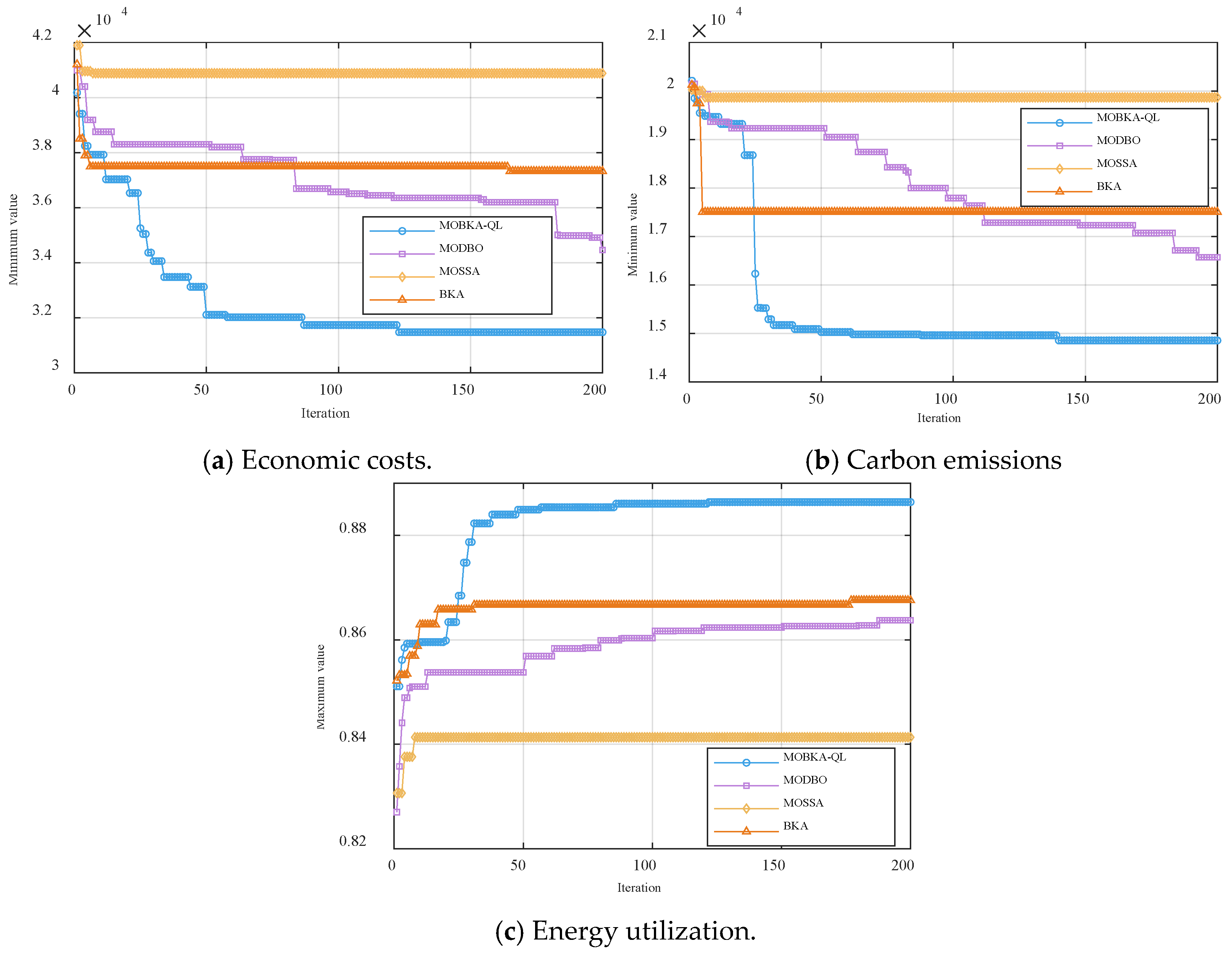
4.3. Algorithm Comparison Test

In this paper, MODBO, MOSSA, and BKA were selected as comparison algorithms to evaluate the performance of MOBKA-QL, which incorporates an adaptive mutation strategy. Using the same model settings, each algorithm was independently executed 50 times to ensure fairness. According to the parameter optimization experiment in Section 3.2, the population size and maximum number of iterations were set to their optimal values. The algorithms’ performance was assessed using five multi-objective evaluation metrics: HV, confidence interval, sample mean, solution running time, and Spread. The running time was averaged over 10 runs.

The test results of the four algorithms under the same model are presented in

Table 6. Calculation of multi-objective evaluation indicators for the four algorithms.

	Confidence Interval			Sample Mean	HV	Time	Spacing
MOBKA-QL	Economic cost	36,920	39,044	37,982	0.0388	244.2983	17,202.8877
	Carbon emission	17,115	18,316	17,716
	Energy efficiency	0.8121	0.82943	0.82076
MODBO	Economic cost	39,006	40,591	39,798	0.0240	476.1714	13,204.9437
	Carbon emission	18,760	19,583	19,171
	Energy efficiency	0.8062	0.8242	0.8152
MOSSA	Economic cost	42,122	42,644	42,383	0.0054	239.0350143	4002.8724
	Carbon emission	20,409	20,737	20,573
	Energy efficiency	0.7982	0.8092	0.8037
BKA	Economic cost	41,076	42,492	41,784	0.0270	238.6687	9745.7401
	Carbon emission	20,304	21,076	20,690
	Energy efficiency	0.7928	0.8228	0.8078

. The test results suggest that MOBKA-QL was completely superior to the other three algorithms in the HV, Spread, and Mean metrics. The confidence interval dominated the other three algorithms. Regardless of some overlap in some objective functions, it did not weaken its overall advantage. The running time of MOBKA-QL (244.2983 s) was slightly slower than that of BKA (238.6687 s). Fortunately, this difference was acceptable considering the algorithm’s improvement in other performance aspects. Thus, the algorithm achieved a preferable balance between solution quality and running efficiency.

The Pareto frontier curves for the optimal solutions of the three objective functions are depicted in Figure 10 to provide a deeper analysis of the four algorithms’ performance. The figure demonstrates that the population distribution of the MOBKA-QL algorithm was more structured and spanned a wider range, showcasing a more balanced advantage across the three dimensions of energy efficiency, carbon emissions, and economic cost. Particularly, the solutions of the MODBO and MOSSA algorithms had a certain degree of concentration regarding energy efficiency and carbon emissions. Nevertheless, their economic costs were not as good as MOBKA-QL, and the population distribution was relatively dispersed. The BKA algorithm also performed well in terms of energy efficiency, whereas its performance concerning carbon emissions and economic costs was suboptimal, resulting in an uneven distribution of its overall solution. This verifies that MOBKA-QL possessed stronger exploration and exploitation capabilities than MODBO, MOSSA, and BKA.

Figure 11 shows the curves of the three objective functions over the number of iterations. At the 200th iteration, MOBKA-QL outperformed the other three algorithms in all three objective functions: economic costs (Figure 11a), carbon emissions (Figure 11b), and energy efficiency utilization rate (Figure 11c). Although MOBKA-QL escaped local optima slightly more slowly than the other algorithms, it showed a clear convergence trend within the first 50 iterations. Overall, MOBKA-QL demonstrated strong global search capabilities and produced superior solutions.

4.4. Model Comparison Test

In this study, a conventional integrated energy system (CIES) without the CCS+P2G model was used as a reference, and the performance improvement of the IES containing the CCS+P2G model was analyzed in depth. Figure 12 illustrates the block diagram of the CIES system. The three objective functions calculated were used to comprehensively evaluate the advantages and disadvantages of both systems, CIES and IES, through comparative analysis.

Three key metrics, energy utilization efficiency (EUE), the carbon dioxide emission reduction rate (CDERR), and the annual total cost savings rate (ATCSR), were adopted in this study to comprehensively assess the system’s performance. The formulas for these metrics are:

$$\left\{\begin{array}{l}ATCSR=(COS{T}_{\mathrm{CIES}}-COS{T}_{\mathrm{IES}})/COS{T}_{\mathrm{CIES}}\\ EUE=(E_{\mathrm{IES}}-E_{\mathrm{CIES}})/E_{\mathrm{CIES}}\\ CDERR=(CD{E}_{\mathrm{CIES}}-CD{E}_{\mathrm{IES}})/CD{E}_{\mathrm{CIES}}\end{array}\right.$$

(39)

where COST represents the economic cost of the system; E denotes the energy utilization efficiency of the system; and CDE indicates the carbon dioxide emissions of the system.

Table 7. Performance metrics for the IES system.

ATCSR	EUE	CDERR
14.63%	28.84%	13.90%

lists the performance metrics of the IES under the optimization model. The data suggest that the IES model introduced in this paper markedly outperformed the traditional IES model in economic, energy efficiency, and environmental benefits, revealing its significant advantages under multi-dimensional optimization.

Figure 13 presents the Pareto frontier of the three objective functions for the CIES and IES systems. Each point represents an optimal solution for the corresponding system. The surface illustrates the confidence regions associated with these optimal solutions, thereby better illustrating the distribution range of the solution sets. The figure indicates that the optimal solution surface of the IES system encompassed that of the CIES system, particularly in the low-carbon emission region. Moreover, the IES system achieved significantly higher energy efficiency and lower economic costs compared to the CIES system. Therefore, the IES system demonstrated significant advantages in overall optimization.

4.5. Operation Strategy Optimization Analysis

The heat-to-power ratio in cogeneration systems is a crucial metric for evaluating both energy efficiency and economic performance. It is essential for the design and optimization of such systems. This paper investigates the operational efficiency and economic benefits of CHP systems under different heat-to-power ratio strategies.

Strategy 1: Electricity determines Heat.

Strategy 2: Heat determines Electricity.

Strategy 3: Adjustable Thermoelectric Ratio.

Using the typical seasonal temperature and energy demand as an example, Figure 14 depicts the temporal variation of the system’s adjustable heat-to-power ratio.

MOBKA-QL was utilized to optimize the system. The Pareto solutions of the IES system under the three strategies are illustrated in Figure 15 (the three-dimensional plots of the three sets of solution sets on the three objective functions (Figure 15d) and two-dimensional plots with different angles (Figure 15a–c). The distribution of the solution sets of the ATR strategy was more concentrated and exhibited stability and equilibrium, so as to have less economic cost and carbon emissions while ensuring higher energy utilization. In contrast, the HDE strategy maintained a good energy utilization rate. Nevertheless, its economic cost and carbon emission performance were poorer. Moreover, the EDH strategy presented a more dispersed solution set distribution, and its energy utilization rate was significantly lower than that of the other two strategies. Hence, the ATR strategy demonstrated significant advantages in multiple objectives.

Five key metrics were utilized to evaluate the performance of the three strategies relative to the CIES system: energy utilization efficiency (EUE), the boiler energy saving rate (BESR), the carbon dioxide emission reduction rate (CDERR), the primary energy saving rate (PESR), and the annual total cost savings rate (ATCSR). The equations are:

$$\left\{\begin{array}{l}BESR=(E{S}_{\mathrm{CIES}}-E{S}_{\mathrm{IES}})/E{S}_{\mathrm{CIES}}\\ PESR=(P{E}_{\mathrm{CIES}}-P{E}_{\mathrm{IES}})/P{E}_{\mathrm{CIES}}\end{array}\right.$$

(40)

where ES represents the boiler energy consumption of the system and PE denotes the primary energy consumption of the system.

Figure 16 presents the evaluation results of the optimal solutions for different strategies. It demonstrates that the adjustable heat-to-power ratio strategy outperformed the constant heat-to-power ratio strategy in terms of EUE, CDERR, and ATCSR. Specifically, the electricity-determined-by-heat strategy achieved the highest BESR at 0.73, due to its prioritization of thermal energy supply, which maximizes boiler energy efficiency. The adjustable heat-to-power ratio strategy had a slightly lower BESR of 0.64 but still showed advantages in overall performance thanks to its flexibility. Regarding PESR, the electric heat strategy reached the highest value of 0.25. Although the adjustable heat-to-power ratio strategy’s economic cost-saving rate was slightly lower at 0.21, it still achieved superior overall economic cost optimization. Overall, the adjustable heat-to-power ratio strategy offers the best trade-off among EUE, ATCSR, and CDERR metrics, demonstrating significantly better comprehensive performance than alternative approaches.

4.6. Analysis of Typical Seasonal Operations

The IES model featuring an adjustable heat-to-power ratio was optimized using MOBKA-QL and TOPSIS. Figure 17 illustrates that the system output primarily supports user-side cooling, heating, and electricity load demands and the energy needs of internal system components.

As demonstrated by the adjustable heat-to-power ratio (Figure 14) and raw operational data (Figure 8), electrical load demand reaches its minimum during nighttime hours while thermal load remains consistently high and stable. During this period, wind turbines achieve peak output in the early night phase, satisfying the majority of power demand. When the system prioritizes CHP operation for thermal load supply, the accompanying electricity generation effectively fills the remaining power gap, resulting in the system’s maximum heat-to-power ratio. During daytime operation, electrical load rises significantly to high levels, coinciding with peak output from solar thermal collectors. Here, the system switches CHP operation to prioritize electricity generation. The relatively small accompanying thermal output is supplemented by gas boilers, thereby reducing the heat-to-power ratio to its minimum value. Throughout this operational cycle, battery storage, thermal energy storage tanks, and the upper-level grid participate in coordinated energy coupling. This multi-agent interaction ensures stable operation of the IES, enabling the efficient collaborative dispatch of multiple energy sources.

When the heat-to-power ratio exceeded 1, the AC served as the primary cooling source, with the EC handling supplementary load. When the ratio fell below 1, the EC assumed the dominant role while the AC provided auxiliary support. This operational strategy, based on heat-to-power ratio characteristics, significantly improved both energy efficiency and economic performance.

Figure 18 presents the action selection frequencies of the Q-learning mechanism during iterative optimization. The convergence of reward curves for all actions reflects the increasing challenge and varying pace in locating optimal solutions through mutation operations. These observations demonstrate the solution set’s asymptotic convergence toward Pareto-optimal solutions.

To visualize optimal CHP dispatch under different scenarios, 17:00 was selected for its representative device operational states. Figure 19 shows real-time energy flows from supply-side sources (wind power, CHP) to demand-side loads (electric/thermal/cooling, storage, and converters) via the multi-energy network. This demonstrates the system’s complexity and flexibility in multi-energy coordination across scenarios.

5. Conclusions

This study constructed an IES coupled with wind and solar energy and developed a dispatch model for this system. The MOBKA-QL algorithm was proposed to solve the optimization problem. Based on five evaluation metrics, the superiority of the IES was verified, the optimal heat-to-power ratio operation strategy was selected, and the stability of the MOBKA-QL algorithm was analyzed. The findings are as follows:

(1)

The proposed IES integrated with CCS+P2G demonstrated significant advantages over CIES during seasonal evaluation, achieving a 14.6% reduction in economic costs, a 13.9% decrease in carbon emissions, and a 28.8% improvement in energy efficiency. These results clearly indicate that the CCS+P2G-enhanced integrated energy system outperforms conventional systems in terms of operational efficiency, energy conservation, emission reduction, and cost-effectiveness. The performance metrics validate the substantial improvements offered by this innovative system configuration compared to traditional approaches.

(2)

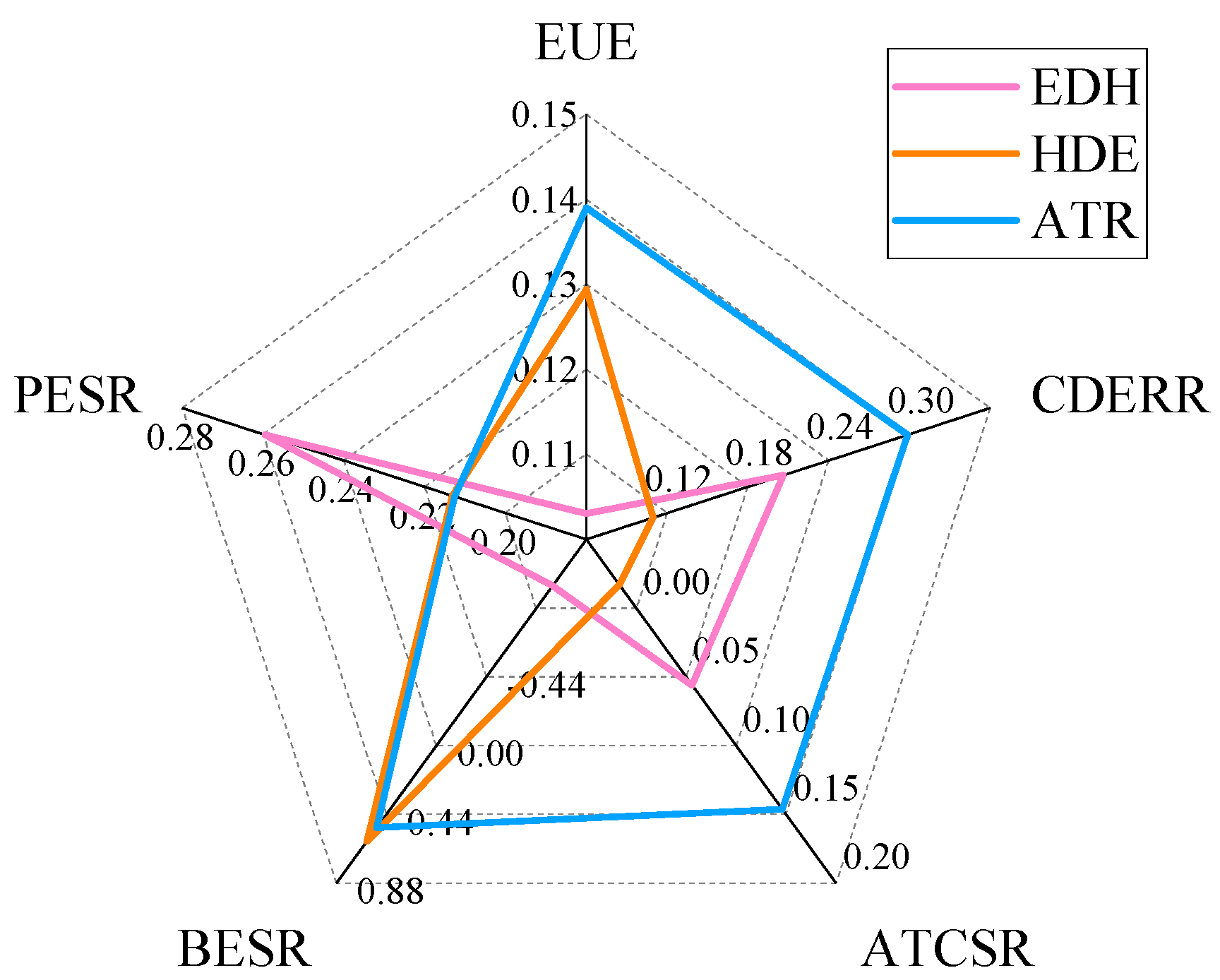
The experimental results for other typical seasons further confirm that the ATR strategy consistently outperformed the constant-ratio strategies. Specifically, compared with the EDH strategy, the ATR strategy reduced economic costs by 9.54%, decreased ${\mathrm{C}\mathrm{O}}_2$ emissions by 11.5%, and improved system energy efficiency by 3.3%. When compared with the HDE strategy, the ATR strategy achieved reductions of 16.1% in economic cost and 20.1% in carbon emissions, along with a 0.8% improvement in energy efficiency. These results demonstrate that the ATR strategy provides significant advantages in minimizing operating costs, reducing environmental impact, and enhancing overall energy performance.

(3)

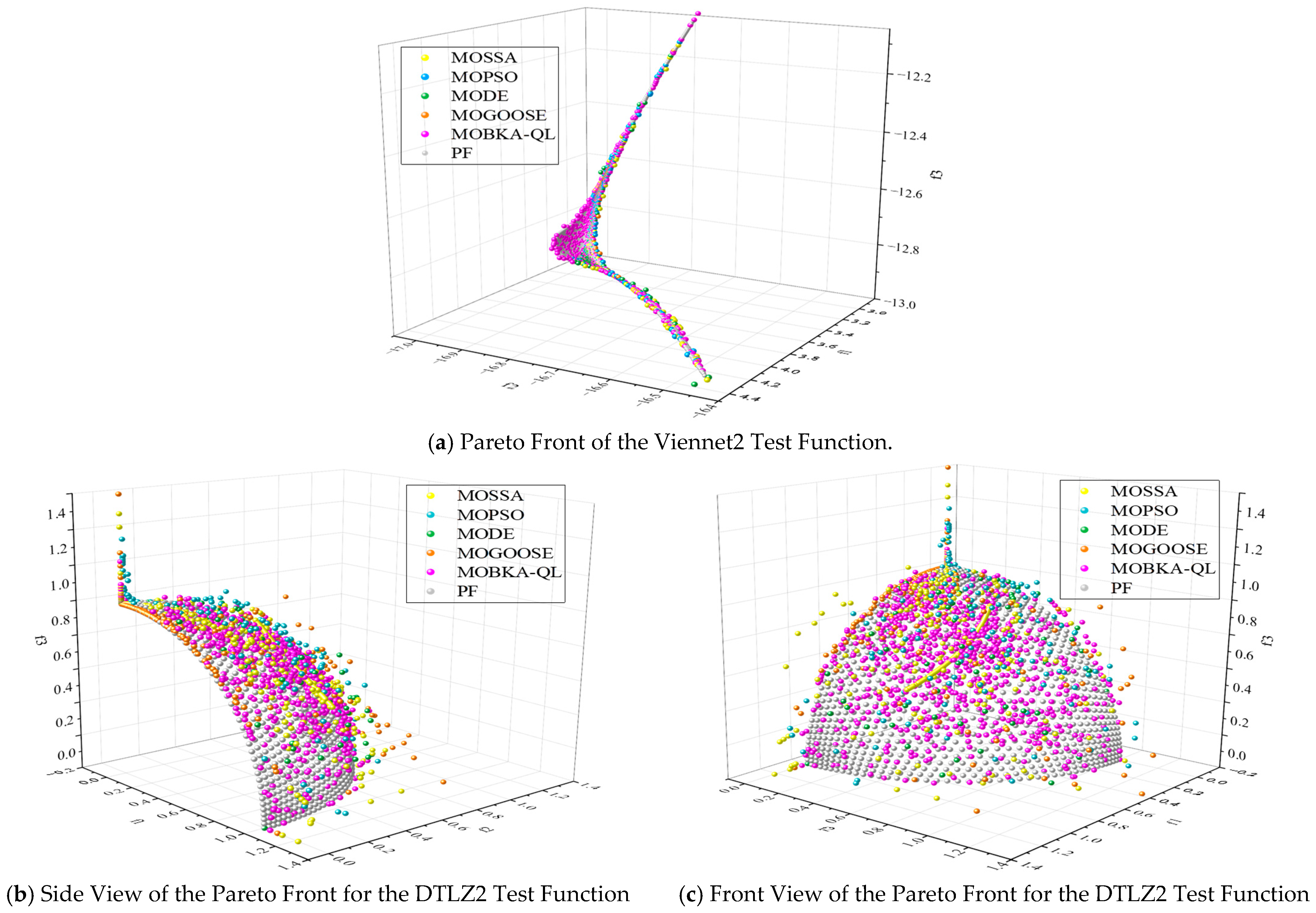
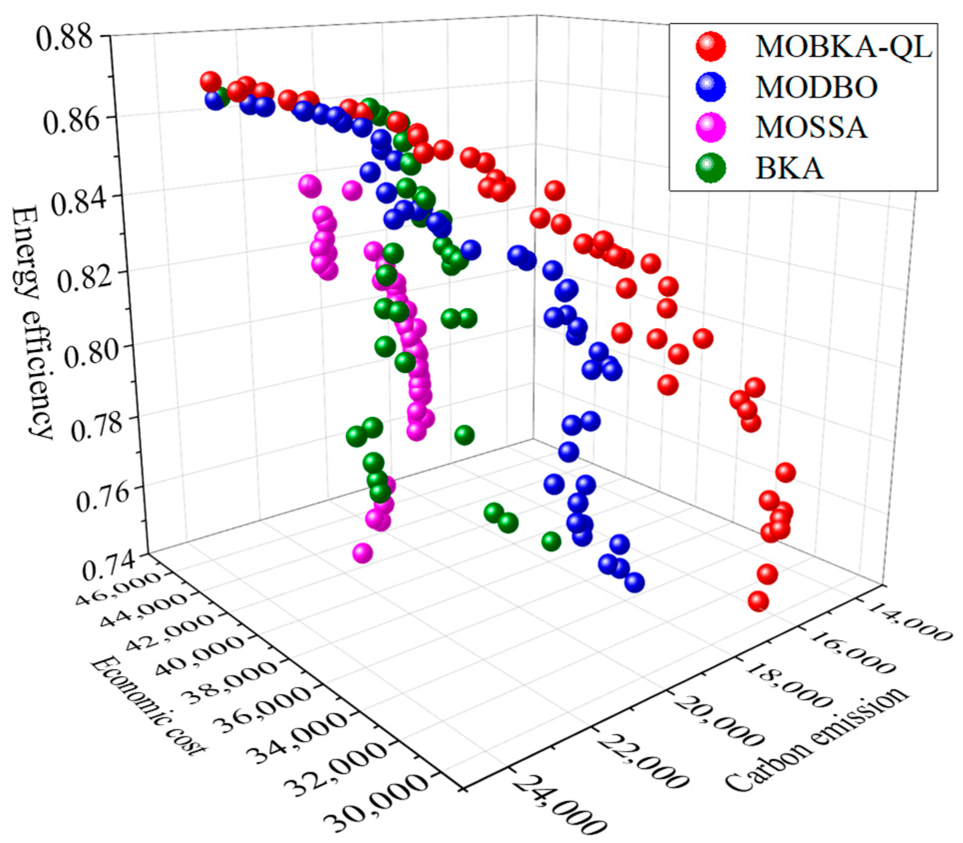
An adaptive mutation strategy based on Q-learning was integrated into the BKA algorithm. Evaluated through MOVI, this approach prevented the population from converging to local optima and increased mutation diversity. Furthermore, multi-objective optimization was applied to enhance the algorithm’s adaptability to complex problems. The results demonstrate that MOBKA-QL outperformed both the original BKA and other representative algorithms (e.g., MOPSO, MODE, and MOSSA, among others) in the IES system, yielding a wider Pareto front and higher solution accuracy, thus confirming its superiority.

However, this study still has certain limitations. For example, the impact of wind power forecast errors has not been systematically considered, the equipment models are relatively simplified, and the generalization ability of the algorithm in complex scenarios requires further validation. In addition, the current research is primarily based on small- to medium-scale systems, and a systematic evaluation of computational scalability and operational efficiency in larger or real-time IES systems is lacking. Future work will focus on enhancing the adaptability and practicality of the algorithm in complex systems, including scenarios such as multi-time-scale scheduling, carbon trading mechanisms, and demand response integration. Meanwhile, the regional adaptability of the model will be assessed under varying energy pricing mechanisms and infrastructure conditions to improve its generalizability.

References

- Ul’yanin, Y.A.; Kharitonov, V.V.; Yurshina, D.Y. Forecasting the dynamics of the depletion of conventional energy resources. Stud. Russ. Econ. Dev. 2018, 29, 153–160. [Google Scholar] [CrossRef]
- Olabi, A.G.; Obaideen, K.; Abdelkareem, M.A.; AlMallahi, M.N.; Shehata, N.; Alami, A.H.; Mdallal, A.; Hassan, A.A.M.; Sayed, E.T. Wind energy contribution to the sustainable development goals: Case study on London array. Sustainability 2023, 15, 4641. [Google Scholar] [CrossRef]
- Pourasl, H.H.; Barenji, R.V.; Khojastehnezhad, V.M. Solar energy status in the world: A comprehensive review. Energy Rep. 2023, 10, 3474–3493. [Google Scholar] [CrossRef]
- Bagherian, M.A.; Mehranzamir, K.; Pour, A.B.; Rezania, S.; Taghavi, E.; Nabipour-Afrouzi, H.; Dalvi-Esfahani, M.; Alizadeh, S.M. Classification and analysis of optimization techniques for integrated energy systems utilizing renewable energy sources: A review for CHP and CCHP systems. Processes 2021, 9, 339. [Google Scholar] [CrossRef]
- Zhao, J.; Luo, X.; Tu, Z.; Chan, S.H. A novel CCHP system based on a closed PEMEC-PEMFC loop with water self-supply. Appl. Energy 2023, 338, 120921. [Google Scholar] [CrossRef]
- Zou, D.; Gong, D.; Ouyang, H. A non-dominated sorting genetic approach using elite crossover for the combined cooling, heating, and power system with three energy storages. Appl. Energy 2023, 329, 120227. [Google Scholar] [CrossRef]
- Pan, C.; Jin, T.; Li, N.; Wang, G.; Hou, X.; Gu, Y. Multi-objective and two-stage optimization study of integrated energy systems considering P2G and integrated demand responses. Energy 2023, 270, 126846. [Google Scholar] [CrossRef]
- Chen, Z.; Yiliang, X.; Hongxia, Z.; Yujie, G.; Xiongwen, Z. Optimal design and performance assessment for a solar powered electricity, heating and hydrogen integrated energy system. Energy 2023, 262, 125453. [Google Scholar] [CrossRef]
- Meng, Q.; Xu, J.; Ge, L.; Wang, Z.; Wang, J.; Xu, L.; Tang, Z. Economic optimization operation approach of integrated energy system considering wind power consumption and flexible load regulation. J. Electr. Eng. Technol. 2024, 19, 209–221. [Google Scholar] [CrossRef]
- Li, Z.; Zhu, X.; Huang, X.; Tian, Y.; Huang, B. Sustainability design and analysis of a regional energy supply CHP system by integrating biomass and solar energy. Sustain. Prod. Consum. 2023, 41, 228–241. [Google Scholar] [CrossRef]
- Zaik, K.; Werle, S. Solar and wind energy in Poland as power sources for electrolysis process-A review of studies and experimental methodology. Int. J. Hydrogen Energy 2023, 48, 11628–11639. [Google Scholar] [CrossRef]
- Li, J.; He, X.; Li, W.; Zhang, M.; Wu, J. Low-carbon optimal learning scheduling of the power system based on carbon capture system and carbon emission flow theory. Electr. Power Syst. Res. 2023, 218, 109215. [Google Scholar] [CrossRef]
- Chen, Z.; Zhang, Y.; Ji, T.; Cai, Z.; Li, L.; Xu, Z. Coordinated optimal dispatch and market equilibrium of integrated electric power and natural gas networks with P2G embedded. J. Mod. Power Syst. Clean Energy 2018, 6, 495–508. [Google Scholar] [CrossRef]
- Calise, F.; Cappiello, F.L.; Cimmino, L.; D’aCcadia, M.D.; Vicidomini, M. Dynamic simulation and thermoeconomic analysis of a power to gas system. Renew. Sustain. Energy Rev. 2023, 187, 113759. [Google Scholar] [CrossRef]
- He, K.; Zeng, L.; Yang, J.; Gong, Y.; Zhang, Z.; Chen, K. Optimization Strategy for Low-Carbon Economy of Integrated Energy System Considering Carbon Capture-Two Stage Power-to-Gas Hydrogen Coupling. Energies 2024, 17, 3205. [Google Scholar] [CrossRef]
- Stecca, M.; Elizondo, L.R.; Soeiro, T.B.; Bauer, P.; Palensky, P. A comprehensive review of the integration of battery energy storage systems into distribution networks. IEEE Open J. Ind. Electron. Soc. 2020, 1, 46–65. [Google Scholar] [CrossRef]
- Hassan, R.; Das, B.K.; Al-Abdeli, Y.M. Investigation of a hybrid renewable-based grid-independent electricity-heat nexus: Impacts of recovery and thermally storing waste heat and electricity. Energy Convers. Manag. 2022, 252, 115073. [Google Scholar] [CrossRef]
- Song, Z.; Liu, T.; Lin, Q. Multi-objective optimization of a solar hybrid CCHP system based on different operation modes. Energy 2020, 206, 118125. [Google Scholar] [CrossRef]
- Xue, J.; Shen, B. A novel swarm intelligence optimization approach: Sparrow search algorithm. Syst. Sci. Control Eng. 2020, 8, 22–34. [Google Scholar] [CrossRef]
- Gen, M.; Lin, L. Genetic algorithms and their applications. In Springer Handbook of Engineering Statistics; Springer: London, UK, 2023; pp. 635–674. [Google Scholar]
- Rana, N.; Latiff, M.S.A.; Abdulhamid, S.M.; Chiroma, H. Whale optimization algorithm: A systematic review of contemporary applications, modifications and developments. Neural Comput. Appl. 2020, 32, 16245–16277. [Google Scholar] [CrossRef]
- Li, L.L.; Ren, X.Y.; Tseng, M.L.; Wu, D.-S.; Lim, M.K. Performance evaluation of solar hybrid combined cooling, heating and power systems: A multi-objective arithmetic optimization algorithm. Energy Convers. Manag. 2022, 258, 115541. [Google Scholar] [CrossRef]
- Yu, H.; Gao, Y.; Wang, J. A multiobjective particle swarm optimization algorithm based on competition mechanism and gaussian variation. Complexity 2020, 2020, 5980504. [Google Scholar] [CrossRef]
- Li, S.; Li, J. Chaotic dung beetle optimization algorithm based on adaptive t-Distribution. In Proceedings of the 2023 IEEE 3rd International Conference on Information Technology, Big Data and Artificial Intelligence (ICIBA), Chongqing, China, 26–28 May 2023; Volume 3, pp. 925–933. [Google Scholar]
- Dong, Y.; Zhang, H.; Wang, C.; Zhou, X. Soft actor-critic DRL algorithm for interval optimal dispatch of integrated energy systems with uncertainty in demand response and renewable energy. Eng. Appl. Artif. Intell. 2024, 127, 107230. [Google Scholar] [CrossRef]
- Suo, L.; Peng, T.; Song, S.; Zhang, C.; Wang, Y.; Fu, Y.; Nazir, M.S. Wind speed prediction by a swarm intelligence based deep learning model via signal decomposition and parameter optimization using improved chimp optimization algorithm. Energy 2023, 276, 127526. [Google Scholar] [CrossRef]
- Li, Y.; Bu, F.; Li, Y.; Long, C. Optimal scheduling of island integrated energy systems considering multi-uncertainties and hydrothermal simultaneous transmission: A deep reinforcement learning approach. Appl. Energy 2023, 333, 120540. [Google Scholar] [CrossRef]
- Chen, L.; Wu, J.; Tang, H.; Jin, F.; Wang, Y. A Q-learning based optimization method of energy management for peak load control of residential areas with CCHP systems. Electr. Power Syst. Res. 2023, 214, 108895. [Google Scholar]
- Dong, Y.; Wang, C.; Zhang, H.; Zhou, X. A novel multi-objective optimization framework for optimal integrated energy system planning with demand response under multiple uncertainties. Inf. Sci. 2024, 663, 120252. [Google Scholar] [CrossRef]
- Wang, J.; Wang, W.; Hu, X.; Qiu, L.; Zang, H.-F. Black-winged kite algorithm: A nature-inspired meta-heuristic for solving benchmark functions and engineering problems. Artif. Intell. Rev. 2024, 57, 98. [Google Scholar] [CrossRef]
- Mohammad, J.; Shahriyar, H.G.; Ata, C.; Song, J.; Markides, C.N. Electrolyzer cell-methanation/Sabatier reactors integration for power-to-gas energy storage: Thermo-economic analysis and multi-objective optimization. Appl. Energy 2023, 329, 120268. [Google Scholar]
- Hu, J.; Zou, Y.; Zhao, Y. Robust operation of hydrogen-fueled power-to-gas system within feasible operating zone considering carbon-dioxide recycling process. Int. J. Hydrogen Energy 2024, 58, 1429–1442. [Google Scholar] [CrossRef]
- Wu, M.; Wu, Z.; Shi, Z. Low carbon economic dispatch of integrated energy systems considering utilization of hydrogen and oxygen energy. Int. J. Electr. Power Energy Syst. 2024, 158, 109923. [Google Scholar] [CrossRef]
- Gao, J.; Meng, Q.; Liu, J.; Wang, Z. Thermoelectric optimization of integrated energy system considering wind-photovoltaic uncertainty, two-stage power-to-gas and ladder-type carbon trading. Renew. Energy 2024, 221, 119806. [Google Scholar] [CrossRef]
- Liang, J.; Tian, M.; Liu, Y.; Zhou, J. Coverage optimization of soil moisture wireless sensor networks based on adaptive Cauchy variant butterfly optimization algorithm. Sci. Rep. 2022, 12, 11687. [Google Scholar] [CrossRef] [PubMed]
- Wen, J.; Wu, X.; Jiang, K.; Cao, B. Particle swarm algorithm based on normal cloud. In Proceedings of the 2008 IEEE Congress on Evolutionary Computation (IEEE World Congress on Computational Intelligence), Hong Kong, China, 1–6 June 2008; pp. 1492–1496. [Google Scholar]
- Cui, L.; Li, G.; Zhu, Z.; Lin, Q.; Wong, K.-C.; Chen, J.; Lu, N.; Lu, J. Adaptive multiple-elites-guided composite differential evolution algorithm with a shift mechanism. Inf. Sci. 2018, 422, 122–143. [Google Scholar] [CrossRef]
- Lin, M.; Wang, Z.; Chen, D.; Zheng, W. Particle swarm-differential evolution algorithm with multiple random mutation. Appl. Soft Comput. 2022, 120, 108640. [Google Scholar] [CrossRef]
- Saadaoui, D.; Elyaqouti, M.; Assalaou, K.; Ben Hmamou, D.; Lidaighbi, S. Parameters optimization of solar PV cell/module using genetic algorithm based on non-uniform mutation. Energy Convers. Manag. X 2021, 12, 100129. [Google Scholar] [CrossRef]
- Ren, X.Y.; Li, L.L.; Ji, B.X.; Liu, J.-Q. Design and analysis of solar hybrid combined cooling, heating and power system: A bi-level optimization model. Energy 2024, 292, 130362. [Google Scholar] [CrossRef]
- Li, Q.; Zeng, X.; Wei, W. Multi-objective particle swarm optimization algorithm using Cauchy mutation and improved crowding distance. Int. J. Intell. Comput. Cybern. 2023, 16, 250–276. [Google Scholar] [CrossRef]
- Yu, H.; Li, J.; Chen, X.; Niu, W.; Sang, H.-Y. An improved multi-objective imperialist competitive algorithm for surgical case scheduling problem with switching and preparation times. Clust. Comput. 2022, 25, 3591–3616. [Google Scholar] [CrossRef]