Abstract
With the emergence of joint business operations involving electric vehicle taxis (EVTs) and charging/swapping stations (CSSTs), a unified decision-making method has become essential for an EVT to select both the driving path and the energy acquisition mode (EAM). The decision making is influenced by energy acquisition cost and potential operation profit. The energy acquisition cost is closely related to the driving time required to reach a CSST, and existing prediction methods for driving time ignore the spatial–temporal interactions of traffic flows on different roads and fail to account for traffic congestion differences across various sections of a road. Existing estimation methods for potential operation income ignore the distributions of taxi orders in different areas. To address these issues, a traffic flow prediction model is first proposed based on the long short-term memory–generative adversarial network (LSTM-GAN) deep learning algorithm. A refined driving time model is developed by segmenting a road into different sections. Then, an expected operation income model is developed considering the distributions of origins and destinations of taxi orders in different areas. Then, a decision-making method for path planning and the charging/swapping mode is proposed, aiming to maximize the total profit of EVTs. Finally, the effectiveness of the proposed decision-making method for EVTs is validated with a city’s traffic network.
1. Introduction
In recent years, electric vehicles (EVs) have been widely deployed owing to their significant advantages in energy conservation and emission reduction [1]. The global number of EVs will increase from 64 million at the end of 2024 to approximately 85 million at the end of 2025, resulting in an average annual growth rate of about 33% [2]. Under this developing trend of vehicles, taxi companies are gradually replacing traditional combustion engine taxis with EV taxis (EVTs) [3,4].
In China, the aim of achieving 100% new energy adoption for EVT deployment is anticipated during the 14th Five-Year Plan period (2021–2025) [5]. An EVT requires electrical energy for driving around. In a few cities, taxi companies have adopted the joint business mode of EVTs and electrical energy supply stations [6]. For instance, in Wuxi City, China, battery swapping stations for EVTs have been applied to establish the business mode [7]. In this business mode, the supply stations and EVT batteries are owned by the taxi company, which sets the energy price and instructs the EVTs to acquire energy at the supply stations. These supply stations, known as charging/swapping stations (CSSTs), offer two energy acquisition modes (EAMs): charging and swapping [8]. The charging mode takes several dozen minutes to complete the energy acquisition, allowing the driver to rest during the charging period. Under the swapping mode, the energy acquisition is quickly completed within a few minutes, thereby increasing the operation time of EVTs [9]. The existing literature compares the socio-economic aspects of the charging mode and swapping mode [10] and examines the economic implications of jointly planning for these two modes [11].
When an EVT with low battery energy aims to drive to a CSST for energy acquisition, the process of driving to the CSST and the choice of the EAM at the CSST significantly impact both energy and time costs [12]. Additionally, the selection of the specific CSST influences the taxi’s future operational income. As the EVT aims to maximize its profit, it encounters the decision-making challenge of determining the optimal driving path to a CSST and which EAM to utilize.
To achieve unified decision making for the selection of the driving path to a CSST and the choice of EAM at the CSST, it becomes essential to evaluate the energy and time costs incurred during the journey to the CSST while adopting the EAM. Furthermore, estimating the future operation income after energy acquisition is also crucial.
The existing literature has investigated decision-making processes concerning the selection of paths for energy acquisition. In ref. [13], a path planning method was introduced, considering the waiting time at the charging station. Ref. [14] proposed a path planning method for EVTs, considering their service level within the traffic network. A path planning method was developed based on the Markov decision process of EVTs, considering the influence of passenger delay [15]. In ref. [16], a path planning method utilizing a probabilistic action tree was proposed to improve EVT income.
However, the income of EVTs is affected by the time and energy costs incurred during the journey to the CSST while executing the EAM. Existing decision-making methods primarily focus on path planning, ignoring the interaction between path planning and the selection of the EAM. Furthermore, these methods have not thoroughly analyzed the different influences of charging and swapping modes on the decision-making process.
The driving time to a CSST serves as a critical factor for path planning, and the driving time can be estimated by predicting the traffic flow. A number of studies have been carried out to investigate the prediction methods for traffic flow. With the assumption of a constant proportion of traffic flow during the same time interval, a traffic flow prediction method was proposed based on the least square fitting method [17]. In ref. [18], the OD matrix was used to predict the traffic flow with an autoregressive model. Based on a multitask learning framework of the deep belief network, a traffic flow prediction method was proposed in [19]. Based on a convolutional long short-term memory (LSTM) neural network, a traffic flow prediction method was proposed in [20].
However, existing traffic flow prediction methods ignore the spatial–temporal interactions of traffic flows on different roads and fail to consider traffic congestion differences across various sections of a road. The prediction error of driving time potentially affects the decision making for path planning.
An EVT aims to choose a CSST that promises higher potential operation income. Several studies have investigated the estimation method for operation income. An income estimation method was developed considering passenger behaviors and energy consumptions along a single road [21]. The income estimation was realized considering the variations in taxi orders within one specific area [22,23].
However, existing income estimation methods primarily focus on taxi orders within a single road or area, neglecting to consider order distributions across different areas.
This paper presents a decision-making method for energy acquisition by EVTs to maximize profits through the joint operation of EVTs and CSSTs. The primary contributions of this paper can be summarized as follows:
- (1)
- Current driving time prediction methods ignore the interactions between adjacent road traffic flows and the differences in traffic congestion among various road sections. Considering the spatial–temporal interactions of traffic flows among different roads, an LSTM–generative adversarial network (LSTM-GAN) deep learning algorithm is developed to predict the traffic flow. Additionally, to create a more detailed model of driving time, roads are segmented into multiple sections based on different speeds. The driving time is finely modeled with time periods of free driving, queueing and intersection passing.
- (2)
- Considering the charging mode and swapping mode, existing operation income estimation methods ignore the interrelationship between the distributions of taxi orders and the energy acquisition mode. Considering the distributions of origin and destination locations of taxi orders in different areas, an expected operation income model is developed to estimate the potential operation income of an EVT with the energy acquisition of charging or swapping at a CSST. The operation income is influenced by both the distributions of taxi orders and the energy acquisition mode.
- (3)
- To describe the combined influence of driving path planning and EAM selection on decision making, the driving time to a CSST and the time required for energy acquisition are estimated by energy cost and income loss. Additionally, the saved charging time under the swapping mode is estimated by energy cost and operation income. To help an EVT achieve the maximum profit, a unified decision-making method is developed by selecting both the driving path to the CSST and the appropriate EAM at the CSST.
The rest of this paper is organized as follows. Section 2 introduces the realization framework of decision making. Section 3 presents the coupled model of the traffic network, CSST and EVT. Section 4 introduces the expected operation income model of EVT. Section 5 introduces the decision-making method. Section 6 presents the study results. Section 7 gives some remarkable conclusion.
2. Framework of Decision Making
Traffic flow reflects the road congestion degree and directly impacts the driving time to a CSST. The time required for finishing charging and swapping is different [9]. The distributions of taxi orders surrounding different CSSTs influence the potential income derived from these orders. Notably, the absence of taxi orders during the driving time to a CSST and the energy acquisition period implies that the driving process, energy acquisition and the destination directly affect the EVT’s profit. Consequently, the operation profit of an EVT is intricately related and constrained by the interaction among the traffic network, CSST, and EVT. Effective decision making for path planning and EAM selection must consider the interdependent characteristics of the traffic network, CSST, and EVT.
The realization framework of the decision-making method for an EVT, aiming at the maximum profit, is shown in Figure 1. When an EVT needs to drive to a CSST for energy acquisition, it transmits information about its current location, initial state of charge (SOC) and battery capacity to the central server. The central server utilizes the LSTM-GAN deep learning algorithm to predict traffic flow, assessing the driving distance and time to the CSST. Then, considering the energy price information, the server evaluates the energy cost incurred during the journey to the CSST and energy acquisition at the CSST. Additionally, it evaluates income loss resulting from the journey time cost to the CSST and the energy acquisition time cost at the CSST. The taxi company transmits the taxi order data to the center server, which estimates the expected income in the future EVT operation period by analyzing the taxi order data. Consequently, the center server helps the EVT make optimal decisions regarding the driving path and EAM at the CSST, providing the recommendation to maximize expected profit.
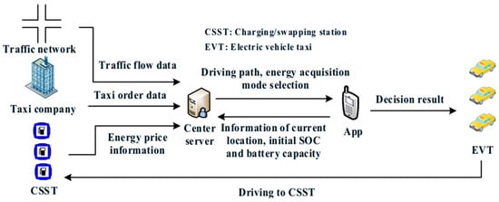
Figure 1.
Realization framework of decision-making method for EVT.
3. Modeling for Traffic Network, CSSTs and EVT
In this section, based on the traditional traffic network topology, the EVT driving time in different sections and different periods is finely divided to form a traffic network topology considering the refined driving time. Furthermore, we analyzed the disparities in driving time costs and charging/swapping costs, taking into account the distinct characteristics of the charging mode and swapping mode and accurately predicting the EVT costs under the charging mode and swapping mode.
3.1. Traffic Network Model
3.1.1. Traffic Network Topology
Considering the road connectivity, the traffic network topology is given by Equation (1) [24].
where represents the topological structure of the traffic network; represents the road node; and are the indices of the road nodes; is the number of road nodes; is the set of all road nodes; represents the road with road nodes and ; is the length of road as given by Equation (2); is the set of all roads; and is the adjacent matrix of as given by Equation (3).
where represents that is not connected to .
where is the actual distance of road .
3.1.2. Modeling for Refined Driving Time
Traffic flow is denoted by the average traffic speed on the road. A specific road can be segmented into several subsections based on varying average traffic speeds within these subsections. Within this context, as traffic flow increases, vehicle speed declines significantly, leading to the formation of queued vehicles. This low-speed condition typically occurs at critical points such as road intersections or segments where traffic demand surpasses road capacity. Such subsections, characterized by low-speed queuing vehicles, are designated as downstream subsections. Conversely, when traffic flow is low, vehicles maintain high speeds without queuing, resulting in unimpeded movement. These subsections, exhibiting high-speed, non-queued traffic, are classified as upstream subsections. Vehicles usually need to wait when driving through an intersection equipped with traffic lights [25]. To account for the distinct traffic speeds across different subsections of the road, the driving time along the road is divided into several time periods, as shown in Figure 2.
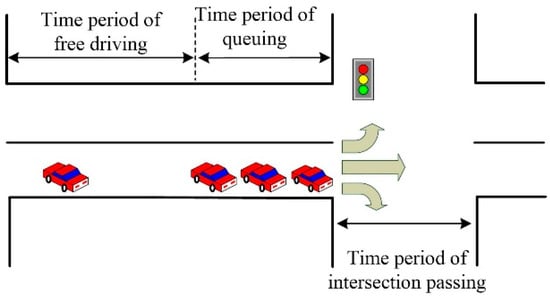
Figure 2.
Division of driving time of EVT.
The driving time of the EVT is defined by Equation (4).
where is the time instant and is the driving time; , and are, respectively, the lengths of time periods of free driving, queueing and intersection passing and are further calculated by Equations (5)–(13).
① Time period of free driving:
As given by Equation (5), is the length of the time period of the vehicle crossing the upstream subsection.
where is the length of queueing vehicles in the downstream subsection and is the average speed on the road.
Then, , as given by Equation (6), is defined as the length of queueing vehicles in the downstream subsection.
where is the number of vehicles on the road; is the average headway of queueing vehicles; is the maximum vehicle flow; and is the green time ratio for the intersection.
Substitute Equation (6) into Equation (5) to obtain Equation (7).
Substitute Equation (7) into Equation (6) to obtain Equation (8).
The road jam density is obtained by the ratio of the maximum vehicle flow over the limited speed on the road. According to the relationship between the road jam density and average speed, is given by Equation (9).
② Time period of queueing:
The time period of queueing is not only determined by the length of queueing vehicles and the maximum vehicle flow on the road but also influenced by the status of traffic lights at the intersection.
When the vehicle arrives at the intersection controlled by a traffic light, the time period of queueing is calculated by Equations (10) and (11).
where is the time period of queueing when the traffic light is green and is the green–red cycle lengths at the intersection.
where is the time period of queueing when the traffic light is red and is the probability of vehicles arriving at the intersection with a green light. is approximated by Equation (12).
③ Time period of intersection passing:
The average length of the time period of vehicles passing through the intersection is given by Equation (13).
where is the time period of finishing the turn or crossing at the intersection.
Therefore, the traffic network topology obtained by considering the refined driving time on the basis of a traditional traffic network is given by Equation (14).
where is the set of the refined driving time on all roads.
3.2. CSST Model
Considering the charging and swapping modes, the CSST model is given by Equations (15) and (16).
where is the set of CSSTs’ locations in the traffic network; is the number of CSSTs; is the index of CSSTs; is the rated charging power of the k-th CSST; is the charging efficiency; is the real-time charging price; is the complete charging/swapping time of EVTs; is defined as the time instants of complete charging, that is, the time instants when the electric vehicle arrives at the CSST plus waiting time and charging time ; is defined as the time instants of complete swapping, that is, the time instants when the electric vehicle arrives at the CSST plus swapping time ; and and are the service cost and energy purchase cost for battery swapping, respectively.
As given by Equation (17), is the arrival time at the CSST of the EVT. The number of EVTs arriving at CSSTs can be predicted. If the number of EVTs that tend to be charged is not greater than the number of chargers, the EVT does not need to wait at the CSST; otherwise, the waiting time at the CSST is given by Equation (18).
where is the time instant when the EVT requires energy acquisition, and is the total driving time of the EVT from initial location to CSST .
where is the set of complete charging time instants of EVTs; is the predicted number of EVTs that will arrived at ; is the number of chargers; and is the number of EVTs waiting at the CSST, where .
3.3. EVT Model
The differences between charging and swapping modes are compared in Figure 3. Upon arrival at a CSST, an EVT has the option to choose between charging or swapping. At the CSST, the EVT opting for charging may undergo waiting and charging time periods, whereas selecting swapping involves only the swapping time period.
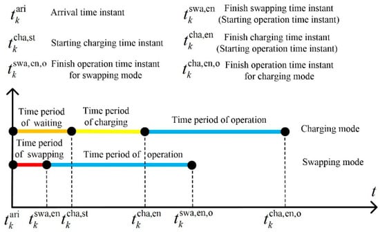
Figure 3.
Comparison of differences between charging and swapping modes.
Due to the significantly shorter swapping time compared to the charging time, the swapping mode effectively saves both the charging and waiting time. The saved time can produce more profit for the EVT. For the charging mode, , and are defined as the time periods of waiting, charging and operation in area , respectively. and are defined as the time instants of start charging and the completed operation time instants for the swapping mode. For the swapping mode, and are defined as the time periods of swapping and operation in area , respectively. is defined as the completed operation time instants for the swapping mode.
Considering charging and driving characteristics, the EVT model is given by Equation (19).
where is the total driving distance of an EVT from initial location to CSST ; is the remaining battery energy of the EVT driving to node ; is the required charging time of the EVT; is the total cost of the EVT in the charging mode, and is the total cost of EVT in the swapping mode.
3.3.1. Driving Distance and Time
The driving distance of the EVT from node to is given by Equations (20) and (21).
where is the binary variable for the road constraint and indicates that the EVT drives through road ; otherwise, is 0.
Thus, the total driving distance and time of the EVT from to CSST are, respectively, given by Equations (22) and (23).
3.3.2. Remaining Battery Energy
The energy consumption of an EVT is influenced by the average driving speed and can be described by a multiple linear regression function [26]. The energy consumption of EVT during the driving process is given by Equation (24).
where is the energy consumption of the EVT during the driving process, and , , and are regression coefficients, which reflect the energy consumption rate and are important for an EVT to make decisions to avoid energy exhaustion.
Based on the energy consumption model, the remaining battery energy of the EVT is given by Equation (25).
where is the energy consumption of the EVT on road ; is the EVT battery capacity; is the SOC of the EVT at node ; is the remaining battery energy when the EVT arrives at a CSST; and is the initial battery energy of the EVT at the initial location for energy acquisition.
3.3.3. Time Period of Charging
Charged battery energy and required charging time of the EVT are given by Equation (26).
where is the SOC of the EVT when charging has finished.
3.3.4. Total Cost Under Charging Mode
The total cost of the EVT (i.e., ) under the charging mode is given by Equation (27).
where the first integral part represents the charging cost for the energy acquisition of the EVT at a CSST, and the second part is the income of the remaining battery energy before charging in the future operation period. We regard the second part as a loss during the EVT charging period, so it is also included in the EVT total charging cost, as detailed in Equation (29). The cost of the remaining battery energy is incorporated in the total cost under the charging mode. This is because that the remaining energy of the EVT can generate income in the future operation period compared to charging.
where is the charging price of the CSST at time instant .
3.3.5. Total Cost Under Swapping Mode
The total cost of an EVT (i.e., ) under the swapping mode is given by Equation (29).
where is the cost of the remaining battery energy before swapping, which is further given by Equation (30).
where is the valley charging price at the CSST.
4. Expected Income Model of EVT
4.1. Traffic Flow Prediction
The traffic flow prediction process is shown in Figure 4. The traffic network matrix sequence contains information about traffic speeds on different roads during different time intervals, and this matrix sequence is transmitted to generator . The matrix sequence is predicted and generated based on multiple training with . Then, the generated matrix sequence is identified by discriminator to judge whether or not the generated matrix sequence is a real matrix sequence. predicts the future traffic flow data by learning the probability distribution from a substantial amount of historical traffic flow data.
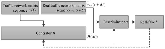
Figure 4.
Process of traffic flow prediction.
The training mechanism of the GAN is shown as follows. If the input of comes from the distribution of the real data, the output of is 1 (real); otherwise, the output is 0 (fake). This can “fool” by producing novel synthesized samples that appear to come from the distribution of the real data. These two mutually adversarial and iterative optimization processes enhance the performance of both and . When cannot correctly identify the fake data generated by and the real ones, it is considered that has learned the distribution of the real data.
As the model of employs the Sigmoid function, the training of involves minimizing its cross entropy. Cross entropy serves as a loss function in machine learning and is used to measure the similarity between the real data distribution and the predicted data distribution of the trained model. This loss function is given by Equation (31).
where is the real data distribution; is the prior distribution; is the time interval; is the probability that comes from the real data; is the generated data coming from ; and is the probability of from .
With generator , Equation (31) is minimized to achieve the optimal solution. In a continuous space, Equation (31) is recast by Equation (32).
For discriminator , the expected output is between 0 and 1. When the input data is sampled from the distribution of the real data, and the goal of is to make output probability close to 1. When the input data are from generated data , tries to correctly judge the data source and makes close to 0, while the goal of is to make close to 1 by iterative training. This means that the data generated by the generator is getting closer and closer to the real data. This is a zero-sum game between and , and the loss function of is . Thus, the objective function of the GAN is given by Equation (33).
The original GAN is augmented by integrating an LSTM network to enable spatial–temporal traffic flow generation. The structure of the LSTM-GAN is shown in Figure 5. The convolution neural network (CNN) layer outputs the features of the data to the LSTM module to learn the temporal characteristics from the spatial correlation characteristics of the historical traffic flow data.
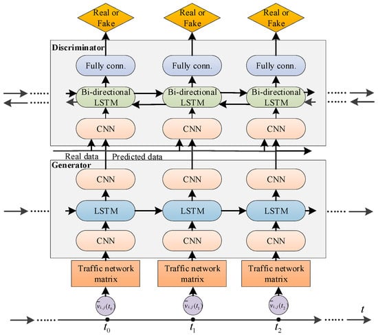
Figure 5.
Structure of LSTM-GAN.
Generator contains three layers to capture the spatial and temporal characteristics of the input traffic flow data:
(1) The observed traffic speed matrix sequence is input into the CNN layer to acquire knowledge regarding the spatial characteristics of the traffic flow data on all roads. (2) The LSTM layer is employed to capture the temporal correlation of the sequential traffic flow data. (3) The output of the LSTM layer is input into another CNN layer to generate the traffic speed matrices during the next time interval.
Discriminator contains three layers, the CNN layer, the bi-directional LSTM layer and the fully connected layer:
(1) The generated and real traffic speed matrices are input into the CNN layer to learn potential spatial features and then are input into a bi-directional LSTM layer to capture the potential temporal features. (2) The fully connected layer is used to transform the output of the bi-directional LSTM layer into a low-dimensional feature vector. (3) The feature vectors are used to construct a classification model to judge the real or fake data of the input future traffic speed matrix.
Thus, the traffic speed data on different roads during the future time period is predicted by the above LSTM-GAN deep learning algorithm.
4.2. Income Calculation of EVT
At different time instants, the distributions of taxi orders in various areas are different. The trajectories for the origin and destination locations of taxi orders reflects the characteristic of traveling behaviors and also reflects the EVT’s potential income across different areas. After the energy acquisition of the EVT at the CSST in a specific area, the EVT aims to obtain income by taking a taxi order around the CSST. The EVT may drive to another area in response to available taxi orders. The expected value of the operation income of the EVT can be evaluated based on the distributions of taxi orders’ origin and destination locations in different areas. To calculate the expected operation income of further operation periods, the unit value of the expected operation income of the EVT is given by Equation (34).
where and are the indices of all areas; means that the EVT drives to area after energy acquisition at the CSST in area ; is the number of areas; is the number of origin locations of taxi orders in area ; is the number of destination locations of taxi orders in area compared to the taxi orders’ origin locations that are in area ; is the average income of the taxi orders whose origin and destination locations are, respectively, in area and area ; is the average operation time of taxi orders whose origin and destination locations are, respectively, in areas and ; and is the unit income of the EVT in area at time instant .
Considering the real-time unit income of an EVT, the expected operation income under the charging mode is the integral of unit income for the further operation period, and the expected operation income under the swapping mode is the integral of unit income and the income gained from the time saved compared to charging. After finishing the energy acquisition at a CSST, the expected income of an EVT in area is given by Equation (35).
where and are the expected operation incomes of the EVT under charging and swapping modes, respectively, and is the expected operation income gained from the time saved with the swapping mode, which is further given by Equation (36).
where is the average unit income of the EVT during a day.
4.3. Income Loss Caused by Driving to CSST
The driving process to the CSST generates no income due to the absence of available taxi orders. The duration of driving time to the CSST is converted to the monetary loss by evaluating the income loss incurred during this driving period. Income loss is evaluated by Equation (37).
5. Modeling for Decision Making
The objective function for maximizing the operation profit of an EVT is given by Equations (38) and (39).
where is the profit of an EVT in the charging mode, and is the profit of EVT in the swapping mode.
The decision making should consider the constraints of road selection, the remaining battery energy and EAM selection.
5.1. Constraint of Road Selection
The EVT drives through the adjacent nodes and ; if is the starting node of the road, then and ; if is the middle node of the road, and is another adjacent node of , then and ; and if is the ending node of the road, then and . Thus, the constraint for road selection is given by Equation (40).
5.2. Constraint of Remaining Battery Energy
When the EVT requires energy acquisition or the battery energy reaches the warning threshold, the app helps the EVT decide how to drive to a CSST. The constraint of the remaining battery energy is given by Equations (41) and (42).
5.3. Constraint of EAM Selection
The constraint of the EAM selection for the EVT is given by Equation (43).
where and are both binary variables. If , the EVT selects charging; otherwise, the EVT selects swapping.
6. Case Studies and Analyses
6.1. Case Scenarios
The traffic network of a city comprising 116 roads is used to verify the proposed decision-making method. The distribution of road nodes, locations of CSSTs, and origin and destination locations of taxi orders are illustrated in Figure 6. Among them, the origin and destination locations of taxi orders are obtained from the analysis of taxi order survey data in a certain region. As can be seen from the figure, the origin location of orders are mostly distributed in residential areas, and the destination location is often concentrated in the work area, while the number of origin and destination locations of orders in commercial areas shows little variation. On weekdays, the peak departure and return times in the residential area occur during 8:00–9:00 and 16:00–18:00, respectively. The peak arrival and departure times in the work area generally span from 9:00 to 10:00 and from 16:00 to 18:00, respectively. The peak arrival time in the commercial area is typically observed from 19:00 to 20:00. The parameter configuration of the LSTM-GAN algorithm in this case study was implemented as follows: the Adam optimization algorithm was employed with a batch size of 64 and a dropout rate of 0.2, and the model was trained for 100 epochs.
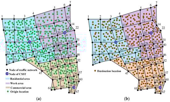
Figure 6.
Distribution of taxi orders in city’s traffic network: (a) origin location distribution; (b) destination location distribution.
The number of chargers, the rated charging power and the charging efficiency of CSSTs are shown in Table 1. The battery capacity, the maximum driving distance and the average headway of queueing vehicles are shown in Table 2. The road parameters are shown in Table 3. The real-time charging price profile of CSSTs is shown in Figure 7. The cost of battery swapping consists of the energy purchase cost of CNY 40 and the service cost of CNY 10. The vehicle speed ranges from 20 to 60 km/h within an urban traffic network. The heuristic ant colony algorithm is used to solve the optimal decision-making problem for the EVT [27].

Table 1.
Parameters of CSSTs.
Table 2.
Parameters of EVT.
Table 3.
Parameters of roads.
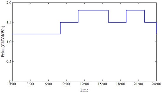
Figure 7.
Real-time charging price profile of CSSTs.
6.2. Study Results
6.2.1. Comparisons of Traffic Flow Prediction Methods
To validate the effectiveness of the proposed LSTM-GAN deep learning algorithm, the mean absolute error (MAE), the mean relative error (MRE), and the root-mean-square error (RMSE) serve as evaluation metrics. Comparative analysis involves comparing the proposed LSTM-GAN against prediction methods such as LSTM [28], ARIMA [29], SVR [30], and the RNN-GAN [31]. As LSTM is a kind of RNN, the RNN-GAN is added as a comparative method to clarify the advantages of the combination of LSTM and the GAN. These methods predict the average speed for the next 15 min, and the comparative results, showing prediction accuracy, are shown in Table 4. It is clear that the proposed LSTM-GAN achieves the lowest MAE, MRE, and RMSE values, attaining the highest prediction accuracy.
Table 4.
Results of different prediction methods.
6.2.2. Decision-Making Results
To verify the effectiveness of the decision-making method, the results for path planning and charging/swapping mode selection are compared under different scenarios. The decision-making time is set at 7:00, node 43 is selected as the initial location, and an initial SOC of 0.3 is selected for decision making. Three scenarios are shown as follows:
Scenario 1: The EVT aims to achieve the maximum profit under this proposed decision-making method.
Scenario 2: The EVT aims to achieve the shortest driving distance to the CSST [32]. The EVT adopts the same EAM as that in scenario 1.
Scenario 3: The EVT aims to achieve the minimum driving time to the CSST [24], also adopting the same EAM as that in scenario 1.
For scenarios 2 and 3, the constraints of road selection and remaining battery energy are assumed to be same as those in scenario 1. Under scenario 1, the result of path planning for EVT is shown in Figure 8. The swapping mode is adopted at node 17, and the path “43 → 44 → 38 → 37 → 36 → 35 → 26 → 17” is selected. The proposed decision-making method for charging/swapping selection is compared to the energy acquisition from charging only. The comparative results are shown in Table 5. Notably, the profits under charging/swapping selection and charging only are CNY 230.79 and CNY 215.82, respectively, while the costs are CNY 86.03 and CNY 74.53, respectively. This indicates that the operation income under charging/swapping selection is higher than that under charging only. This is because the income loss of swapping is less than that of charging and the saved time generates more income. To verify the effectiveness of the proposed LSTM-GAN algorithm in saving the cost of the EVT, the comparison result of the average energy acquisition costs under different prediction methods is shown in Table 6. It is obvious that the proposed LSTM-GAN algorithm has the lowest cost for energy acquisition.
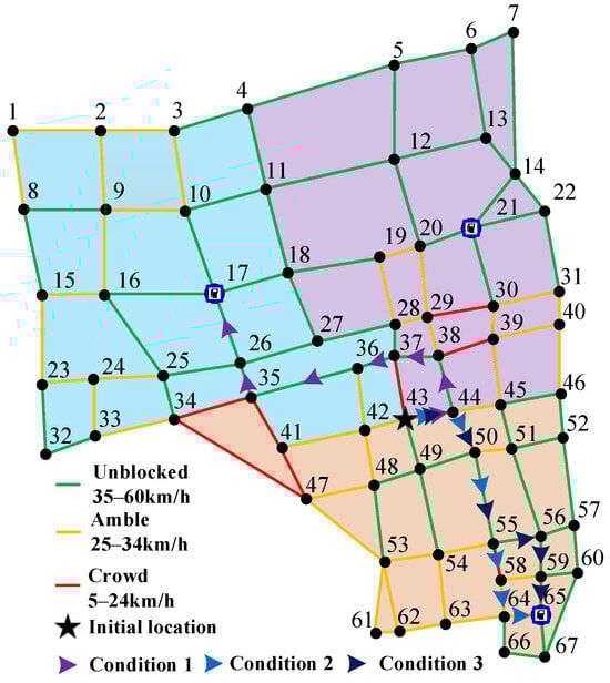
Figure 8.
Path planning of EVT under different scenarios.
Table 5.
Results under different EAMs.
Table 6.
Cost comparison of different prediction methods.
Under scenarios 2 and 3, the results of path planning are shown in Figure 8. Under scenario 2, the shortest path is “43 → 44 → 50 → 55 → 58 → 64 → 65”. The path with the minimum driving time is “43 → 44 → 50 → 55 → 56 → 59 → 65” in scenario 3. Comparative results under the three scenarios are shown in Table 7. The EVT in scenario 1 did not select the path with the shortest driving distance or minimal driving time. However, this suboptimal route was ultimately chosen by the EVT due to its capacity to maximize profit during future operational periods. This is because the shortest driving path distance and the minimum driving time only impact the cost of the energy consumption during the driving process to CSST. The low cost does not mean high operation income. The expected profit of the EVT is also influenced by expected operation income from taxi orders. In scenario 1, the EVT selects the CSST in the area with more taxi orders in the future operation period, which helps the EVT obtain higher income compared to the other two scenarios. Thus, the proposed method helps the EVT make decisions regarding path planning and charging/swapping mode selection to maximize profit.
Table 7.
Results of EVT under three scenarios.
6.2.3. Decision-Making Results with Different Factors
- ①
- Decision making under different initial SOCs:
The decision-making results with different initial SOCs at 7:00 and node 43 are shown in Figure 9 and Table 8. When the initial SOC is higher than 0.1, the EVT selects the same path as in scenario 1. When the initial SOC is equal to 0.1, the selected path is “43 → 37 → 28 → 19 → 20 → 21”, and the profit of the EVT is lower than that when the initial SOC is 0.2. This is because the EVT is constrained by the remaining battery energy and cannot select the path for the maximum profit of the EVT. The EVT can only select the path with the shortest distance with congested traffic.
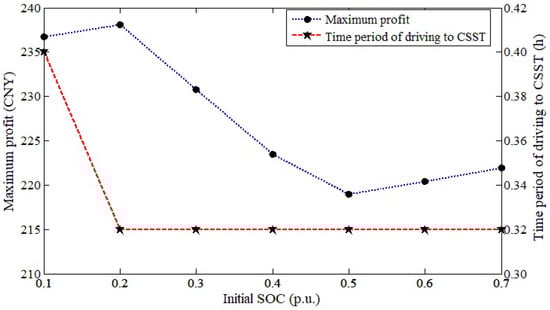
Figure 9.
Maximum profit of EVT under different initial SOCs.
Table 8.
Results under different initial SOCs.
When the initial SOC is 0.1, the difference between the optimal operation profits with the swapping/charging mode and charging only reaches a maximum value of CNY 34.93. When the initial SOC is less than 0.5, the optimal EAM for the EVT is swapping. When the initial SOC is low, the income loss of swapping is less than that of charging, and the saved time generates higher income. Thus, the EVT obtains the maximum profit under swapping. With the increase in the initial SOC, the cost of charging is much lower than that of swapping. When the SOC is low, the EVT is recommended to select the swapping mode.
- ②
- Decision making under different time instants:
Figure 10 and Table 9 present the results at different decision-making time instants at node 43 when the EVT’s initial SOC is 0.3. It is clear that the EVT selects different paths at different times, leading to variations in profit and driving time due to different traffic congestions and taxi order distributions. The EVT achieves the lowest and highest profits at 9:00 and 14:00, respectively. This is because the time period after 14:00 is the peak off-duty period, during which the EVT receives more orders than other time periods. Thus, the time chosen for decision making significantly influences the EVT’s operation profit, and the decision is recommended to be made before the peak off-duty period.
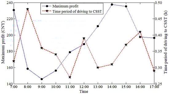
Figure 10.
Maximum profit of EVT under different decision-making time instants.
Table 9.
Results under different decision-making time instants.
- ③
- Decision making at different initial locations:
Figure 11 presents the results at different initial locations among three areas and under different initial SOCs at 7:00. Table 10 provides comparative results of profits and paths at different initial locations among three areas for decision making at 7:00 with the initial SOC of 0.3. It is clear that there is a general decrease in the maximum profit of the EVT from area 1 to area 3. The EVT’s profit decreases with the increase in the initial SOC. This is because the EVT tends to achieve higher profit when the initial location is closer to the area with more intensive taxi orders. The profits of the EVT at different locations within an individual area show fluctuations. This is because the EVT selects different driving paths based on the various road congestion degrees. Therefore, different initial locations for decision making significantly influence the profit of the EVT in the future operation period.
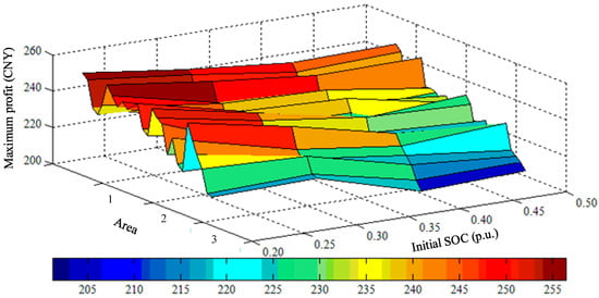
Figure 11.
Maximum profit of EVT at different initial locations among three areas and under different initial SOCs for decision making.
Table 10.
Results with different initial locations for decision making.
7. Conclusions
With the joint operation of EVTs and CSSTs, a decision-making method for the energy acquisition of an EVT is proposed to achieve the maximum profit. Specific conclusions are summarized as follows:
- (1)
- The proposed decision-making method significantly aids the EVT in achieving maximum profit by enabling unified decision making for the driving path to a CSST and the selection of an EAM. Compared to the charging mode, the operation profit of the EVT is increased with charging/swapping selection.
- (2)
- The traffic flow prediction method is developed based on the LSTM-GAN deep learning algorithm. The mean relative error for the traffic flow prediction decreases to 8.38%. Considering the traffic congestion differences in different subsections of an individual road, a traffic network model is developed with a refined driving time for the EVT. When an EVT decides to drive to a CSST, the traffic flow prediction and refined driving time improve calculation accuracy for the decision making.
- (3)
- Considering the variations in the distributions of taxi orders’ origin and destination locations in different areas, an expected operation income model of an EVT is developed. This proposed model facilitates EVTs in evaluating the potential operation income under the driving path to a CSST and the alternate EAM selections post arrival at the CSST. The results show that the driving path chosen by EVTs may not be the optimal path with the shortest driving time or the shortest driving distance but the suboptimal path with the greatest profit.
This paper solely focuses on the application of the LSTM-GAN traffic flow prediction model and decision-making approach proposed herein, specifically in the context of taxi operations and profitability within a scenario where charging and swapping modes coexist. Although only one type of electric vehicle is considered in this paper, the model and algorithm proposed in this paper can be applied to other types of vehicles and cities. Future research could expand on this by exploring various types of electric vehicles, such as examining their potential to decrease power replenishment cost for electric private cars and enhance the operational income of electric buses, among other applications. Furthermore, future research could examine the applicability of the proposed model and strategy in dynamic traffic environments, as well as their performance variations when implemented in different urban settings.
Author Contributions
Conceptualization, L.C., H.Q. and M.W.; methodology, L.C., Y.L. and Q.W.; software, L.C. and Q.W.; validation, L.C., H.Q. and Q.W.; formal analysis, L.C. and H.Q.; data curation, Y.L., M.W. and Q.W.; writing—original draft preparation, L.C. and Q.W.; writing—review and editing, Y.L., Y.W. and M.W.; visualization, Y.W., M.W. and Q.W.; resources, supervision, project administration, funding acquisition, H.Q., M.W. and Y.W. All authors have read and agreed to the published version of the manuscript.
Funding
This research was funded by Jiangsu Province Youth Science and Technology Talent Support Project with grant number JSTJ-2024-053.
Institutional Review Board Statement
Not applicable.
Informed Consent Statement
Not applicable.
Data Availability Statement
The data presented in this study are available on request from the corresponding author.
Conflicts of Interest
The authors declare no conflicts of interest.
Nomenclature
| Abbreviations: | |||
| CSST | Charging/swapping station. | EVT | Electric vehicle taxi. |
| LSTM-GAN | Long short-term memory–generative adversarial network. | SOC | State of charge. |
| EAM | Energy acquisition mode. | ||
| Sets and Indices: | |||
| Set of CSST’s location, rated fast charging power, charging efficiency and price. | Set of EVT’s driving distance, time periods, remaining battery energy and costs. | ||
| Topological structure of the traffic network. | Set of initial locations of EVT. | ||
| Set of all roads. | Set of CSSTs’ locations in the traffic network. | ||
| Set of refined time periods of driving through all roads. | Adjacent matrix of the length of road. | ||
| Set of all road nodes. | Length of road . | ||
| Index of all areas. | Time period of operation in area for charging mode (h). | ||
| EVT drives to area after energy acquisition at CSST in area . | Number of areas. | ||
| Index of road nodes. | Time instant. | ||
| Index of CSSTs. | Number of EVTs waiting at CSST. | ||
| m | Number of CSSTs. | Number of fast chargers. | |
| n | Number of road nodes. | ||
| Parameters: | |||
| Energy purchase cost for battery swapping (CNY). | Time period of operation in area for swapping mode (h). | ||
| Valley charging price at CSST (CNY/kWh). | Time period of waiting for charging mode (h). | ||
| Service cost for battery swapping (CNY/kWh). | Time period of queueing when the traffic light is green (h). | ||
| Actual distance of road (km). | Time period of queueing when the traffic light is red (h). | ||
| Completed charging/swapping time of EVTs. | Arrival time of EVT to CSST. | ||
| Battery capacity of EVT (kWh). | Complete charging time instant (i.e., starting operation time instant) for charging mode. | ||
| Initial battery energy of EVT at the initial location (kWh). | Complete operation time instant for charging mode. | ||
| Average headway of queueing vehicles (m/Veh.). | Starting charging time instant for charging mode. | ||
| Average income of the taxi orders whose origin and destination locations are, respectively, in area and area (CNY). | Complete swapping time instant (i.e., starting operation time instant) for swapping mode. | ||
| Probability of vehicles arriving at the intersection during a green light. | Complete operation time instant for swapping mode. | ||
| Rated fast charging power of the k-th CSST (kW). | Time instant when the EVT requires energy acquisition. | ||
| Time period of charging for charging mode (h). | / | Road node /. | |
| Time period of swapping for swapping mode (h). | Limited speed on the road (km/h). | ||
| Maximum vehicle flow (Veh./h). | Green and red cycle lengths (s). | ||
| Green time ratio. | Average unit income of EVT during a day (CNY/h). | ||
| Charging efficiency. | Time interval (h). | ||
| Variables: | |||
| Total cost of EVT under the charging mode (CNY). | Number of origin locations of taxi orders in area . | ||
| Monetary cost caused by driving to CSST (CNY). | Number of vehicles on the road (Veh.). | ||
| Total cost of EVT under the swapping mode (CNY). | Predicted number of EVTs that will arrived at (Veh.). | ||
| Real-time charging price (CNY/kWh). | SOC of EVT at node (p.u.). | ||
| Energy consumption of EVT (kWh/km). | SOC of EVT when charging has finished (p.u.). | ||
| Energy consumption of EVT on road (kWh). | Total driving time of EVT from initial location to CSST (h). | ||
| Remaining battery energy of EVT driving to node (kWh). | Driving time (h). | ||
| Charged battery energy (kWh). | Time period of free driving (h). | ||
| Remaining battery energy when EVT arrives at CSST (kWh). | Time period of queueing (h). | ||
| Total driving distance of EVT from initial location to CSST (km). | Time period of intersection passing (h). | ||
| Driving distance of EVT from node to node (km). | Required charging time of EVT (h). | ||
| Length of the queueing vehicles in downstream subsection (km). | Average speed of vehicles on the road (km/h). | ||
| Expected operation income of EVT under charging mode (CNY). | Profit under charging mode (CNY). | ||
| Expected operation income under the saved time with swapping mode (CNY). | Profit under swapping mode (CNY). | ||
| Expected operation income of EVT under swapping mode (CNY). | Binary variable for road constraint. | ||
| Number of destination locations of taxi orders in area compared to taxi orders’ origin locations in area . | Time period of completing the turn at the intersection (h). | ||
| Maximum operation profit of EVT (CNY). | |||
References
- Lakatos, I. Economic and ecological aspects of vehicle diagnostics. Sustainability 2025, 17, 1662. [Google Scholar] [CrossRef]
- Forecast Analysis: Electric Vehicle Shipments, Worldwide. Available online: https://www.gartner.com/en/documents/6008203 (accessed on 31 March 2025).
- Wang, H.; Zhao, D.; Cai, Y.; Li, J.; Chen, S. Taxi trajectory data based fast-charging facility planning for urban electric taxi systems. Appl. Energy 2021, 286, 116515. [Google Scholar] [CrossRef]
- Yun, B.; Sun, D.; Zhang, Y.; Deng, S.; Xiong, J. A charging location choice model for plug-in hybrid electric vehicle users. Sustainability 2019, 11, 5761. [Google Scholar] [CrossRef]
- Zhao, Z.; Tian, D.; Duan, X.; Duan, L.; Zhang, P.; Li, W. Joint optimization of battery swapping scheduling for electric taxis. Sustainability 2023, 15, 13722. [Google Scholar] [CrossRef]
- Huang, Y.; Hu, H.; Tan, J.; Xuan, D. Deep reinforcement learning based energy management strategy for range extend fuel cell hybrid electric vehicle. Energy Convers. Manag. 2023, 277, 116678. [Google Scholar] [CrossRef]
- Circular of the General Office of the Municipal Government on Printing and Issuing the Planning of Charging and Replacing Facilities for New Energy Vehicles in Wuxi City During the 14th Five-Year Plan Period. Available online: https://www.wuxi.gov.cn/doc/2022/06/29/3702607.shtml (accessed on 31 March 2025).
- Zhang, T.; Huang, Y.; Liao, H.; Liang, Y. A hybrid electric vehicle load classification and forecasting approach based on GBDT algorithm and temporal convolutional network. Appl. Energy 2023, 351, 121955. [Google Scholar] [CrossRef]
- Wang, A. Economic efficiency of high-performance electric vehicle operation based on neural network algorithm. Comput. Electr. Eng. 2023, 112, 104589. [Google Scholar]
- Gao, J.; Li, S. Charging autonomous electric vehicle fleet for mobility-on-demand services: Plug in or swap out? Transp. Res. Part C Emerg. Technol. 2024, 158, 104457. [Google Scholar] [CrossRef]
- Lai, Z.J.; Li, S. Towards a multimodal charging network: Joint planning of charging stations and battery swapping stations for electrified ride-hailing fleets. Transport. Res. B-Meth. 2024, 183, 102928. [Google Scholar] [CrossRef]
- Arif, S.M.; Lie, T.T.; Seet, B.C.; Ayyadi, S.; Jensen, K. Review of electric vehicle technologies, charging methods, standards and optimization techniques. Electronics 2021, 10, 1910. [Google Scholar] [CrossRef]
- Yao, Z.; Wang, Z.; Ran, L. Smart charging and discharging of electric vehicles based on multi-objective robust optimization in smart cities. Appl. Energy 2023, 343, 121314. [Google Scholar] [CrossRef]
- Liang, Y.; Wang, H.; Zhao, X. Analysis of factors affecting economic operation of electric vehicle charging station based on DEMATEL-ISM. Comput. Ind. Eng. 2023, 163, 108455. [Google Scholar] [CrossRef]
- Sayarshad, H.R.; Mahmoodian, V.; Oliver, H.G. Non-myopic dynamic routing of electric taxis with battery swapping stations. Sustain. Cities Soc. 2020, 57, 102113. [Google Scholar] [CrossRef]
- Tu, W.; Mai, K.; Zhang, Y. Real-time route recommendations for e-taxis leveraging GPS trajectories. IEEE Trans. Ind. Inf. 2020, 17, 3133–3142. [Google Scholar] [CrossRef]
- Lee, S.; Choi, D.H. Dynamic pricing and energy management for profit maximization in multiple smart electric vehicle charging stations: A privacy-preserving deep reinforcement learning approach. Appl. Energy 2021, 304, 117738. [Google Scholar] [CrossRef]
- Aljafari, B.; Jeyaraj, P.R.; Kathiresan, A.C.; Thanikanti, S.B. Electric vehicle optimum charging-discharging scheduling with dynamic pricing employing multi-agent deep neural network. Comput. Electr. Eng. 2023, 105, 108555. [Google Scholar] [CrossRef]
- Wang, K.; Wang, H.; Yang, Z.; Feng, J.; Li, Y.; Yang, J.; Chen, Z. A transfer learning method for electric vehicles charging strategy based on deep reinforcement learning. Appl. Energy 2023, 343, 121186. [Google Scholar] [CrossRef]
- Ma, Y.; Zhang, Z.; Ihler, A. Multi-lane short-term traffic forecasting with convolutional LSTM network. IEEE Access 2020, 8, 34629–34643. [Google Scholar] [CrossRef]
- Ren, L.; Yuan, M.M.; Jiao, X.H. Electric vehicle charging and discharging scheduling strategy based on dynamic electricity price. Eng. Appl. Artif. Intell. 2023, 123, 106320. [Google Scholar] [CrossRef]
- Zhang, D.; Sun, L.; Li, B.; Chen, C.; Pan, G.; Li, S.; Wu, Z. Understanding taxi service strategies from taxi GPS traces. IEEE Trans. Intell. Transp. Syst. 2014, 16, 123–135. [Google Scholar] [CrossRef]
- Qin, G.; Li, T.; Yu, B.; Wang, Y.; Huang, Z.; Sun, J. Mining factors affecting taxi drivers’ incomes using GPS trajectories. Transp. Res. Part C Emerg. Technol. 2017, 79, 103–118. [Google Scholar] [CrossRef]
- Xing, Q.; Chen, Z.; Zhang, Z.; Huang, X.; Leng, Z.; Sun, K.; Chen, Y.; Wang, H. Charging demand forecasting model for electric vehicles based on online ride-hailing trip data. IEEE Access 2019, 7, 137390–137409. [Google Scholar] [CrossRef]
- Fayazi, S.A.; Vahidi, A. Crowdsourcing phase and timing of pre-timed traffic signals in the presence of queues: Algorithms and back-end system architecture. IEEE Trans. Intell. Transp. Syst. 2016, 17, 870–881. [Google Scholar] [CrossRef]
- Guo, Q.; Xin, S.; Sun, H.; Li, Z.; Zhang, B. Rapid-charging navigation of electric vehicles based on real-time power systems and traffic data. IEEE Trans. Smart Grid 2014, 5, 1969–1979. [Google Scholar] [CrossRef]
- Liao, E.; Liu, C. A hierarchical algorithm based on density peaks clustering and ant colony optimization for traveling salesman problem. IEEE Access 2018, 6, 38921–38933. [Google Scholar] [CrossRef]
- Tian, Y.; Zhang, K.; Li, J.; Lin, X.; Yang, B. LSTM-based traffic flow prediction with missing data. Neurocomputing 2018, 318, 297–305. [Google Scholar] [CrossRef]
- Hou, Q.; Leng, J.; Ma, G.; Liu, W.; Cheng, Y. An adaptive hybrid model for short-term urban traffic flow prediction. Phys. A Stat. Mech. Appl. 2019, 527, 121065. [Google Scholar] [CrossRef]
- Wang, D.; Wang, C.; Xiao, J.; Li, Y.; Zhang, H. Bayesian optimization of support vector machine for regression prediction of short-term traffic flow. Intell. Data Anal. 2019, 23, 481–497. [Google Scholar] [CrossRef]
- Kim, J.; Lee, C. Deep unsupervised learning of turbulence for inflow generation at various reynolds numbers. J. Comput. Phys. 2020, 406, 109216. [Google Scholar] [CrossRef]
- Morlock, F.; Rolle, B.; Bauer, M.; Sawodny, O. Time optimal routing of electric vehicles under consideration of available charging infrastructure and a detailed consumption model. IEEE Trans. Intell. Transp. Syst. 2020, 21, 5123–5135. [Google Scholar] [CrossRef]
Disclaimer/Publisher’s Note: The statements, opinions and data contained in all publications are solely those of the individual author(s) and contributor(s) and not of MDPI and/or the editor(s). MDPI and/or the editor(s) disclaim responsibility for any injury to people or property resulting from any ideas, methods, instructions or products referred to in the content. |
© 2025 by the authors. Licensee MDPI, Basel, Switzerland. This article is an open access article distributed under the terms and conditions of the Creative Commons Attribution (CC BY) license (https://creativecommons.org/licenses/by/4.0/).