
A Pricing Strategy for Key Customers: A Method Considering Disaster Outage Compensation and System Stability Penalty


Abstract
1. Introduction
2. Related Work
- It presents a two-stage optimization framework that utilizes second-order conic programming (SOCP) for normal operations and mixed-integer second-order conic programming (MISOCP) for rescheduling during outage scenarios, ensuring optimal dispatch of BESS and hydrogen energy storage systems (HESS) while considering load shedding.
- It quantifies the unsupplied power demand and voltage impacts when critical loads are prioritized in isolated networks, thereby reflecting both outage compensation and grid stability concerns.
- It proposes a novel pricing model for key customers that incorporates additional costs associated with disaster-induced outages and voltage degradation, promoting fair and balanced contractual negotiations.
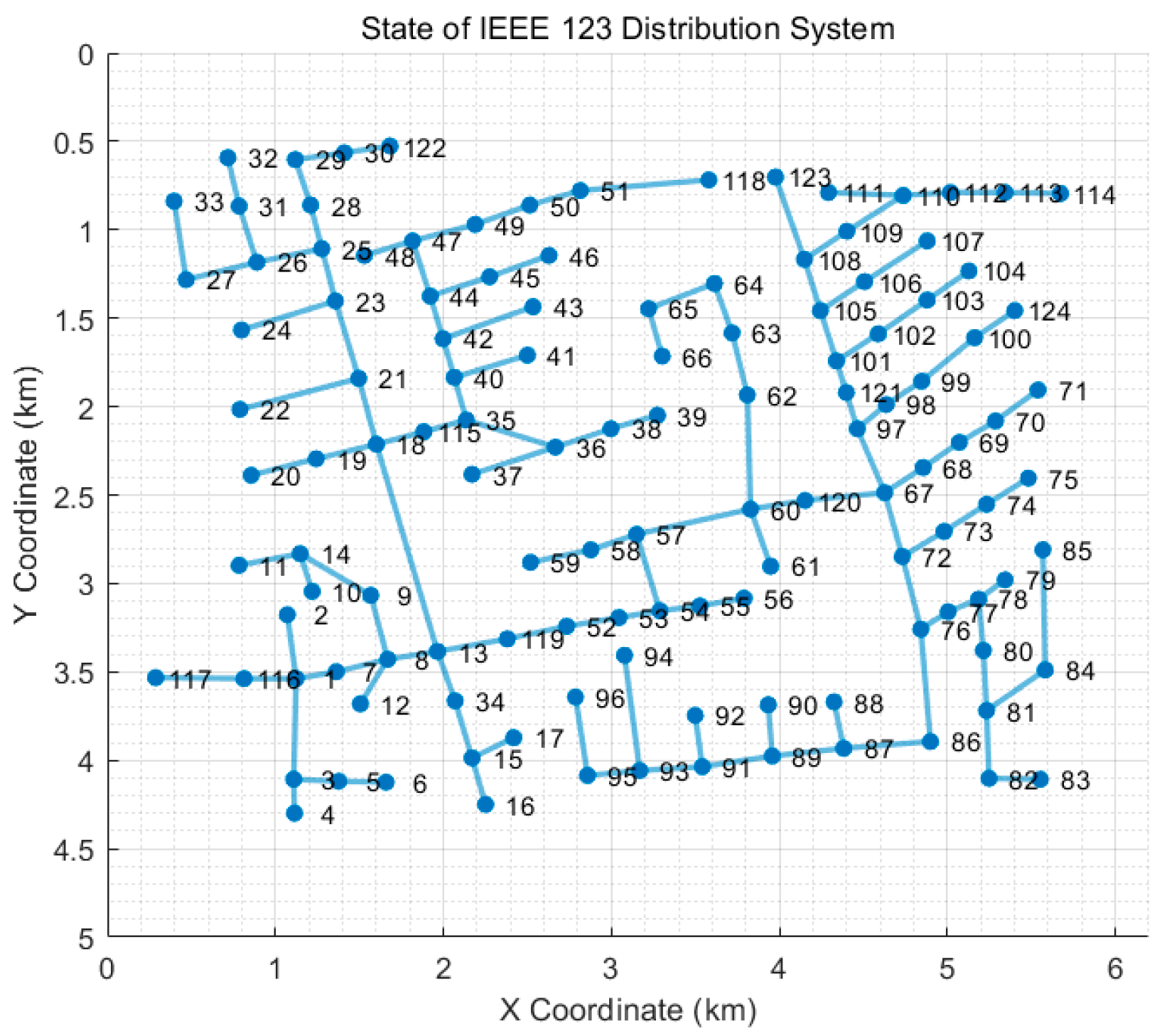
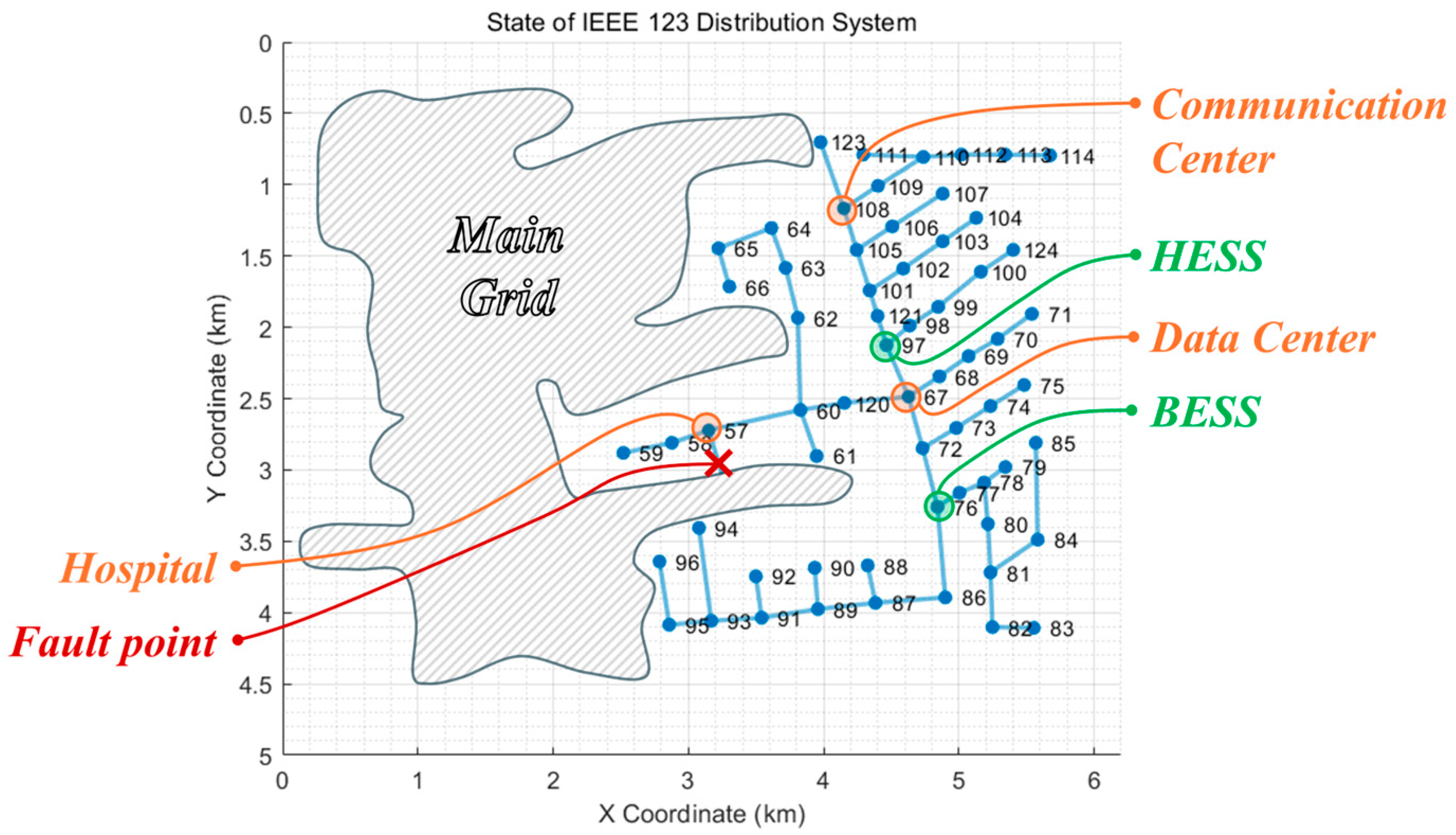
- It demonstrates the practical application of the methodology through a case study using the IEEE 123 bus test node system, validating the proposed approach with realistic load and generation profiles.
3. Methodology and Problem
3.1. Overall Process
3.2. Microgrid Optimal Day-Ahead Scheduling
3.2.1. Objective Function
3.2.2. Power Flow and Power Balance Constraints
3.2.3. Bus Voltage and Line Current Constraints
3.2.4. Active/Reactive Power Ratio
3.2.5. Electricity Trade with the Main Grid
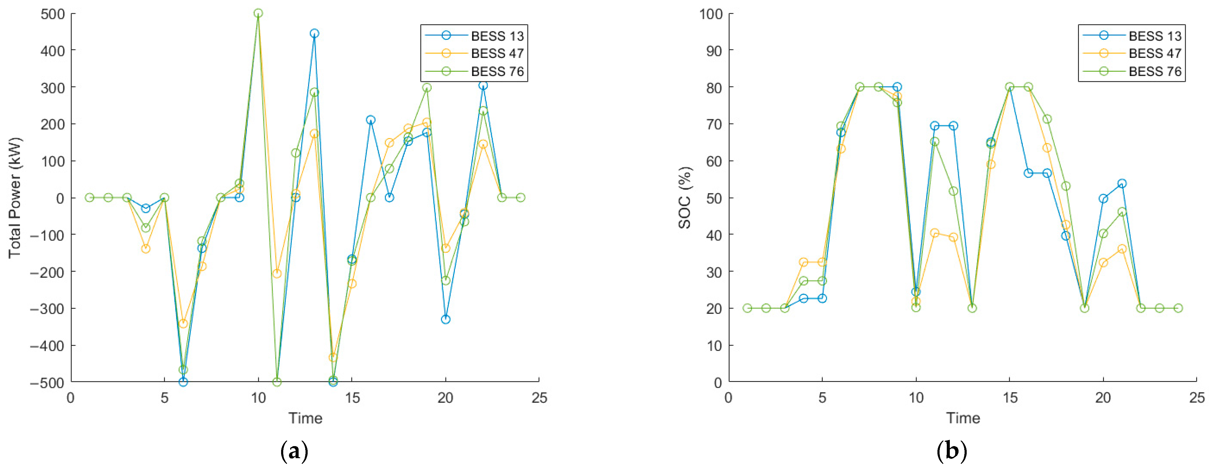
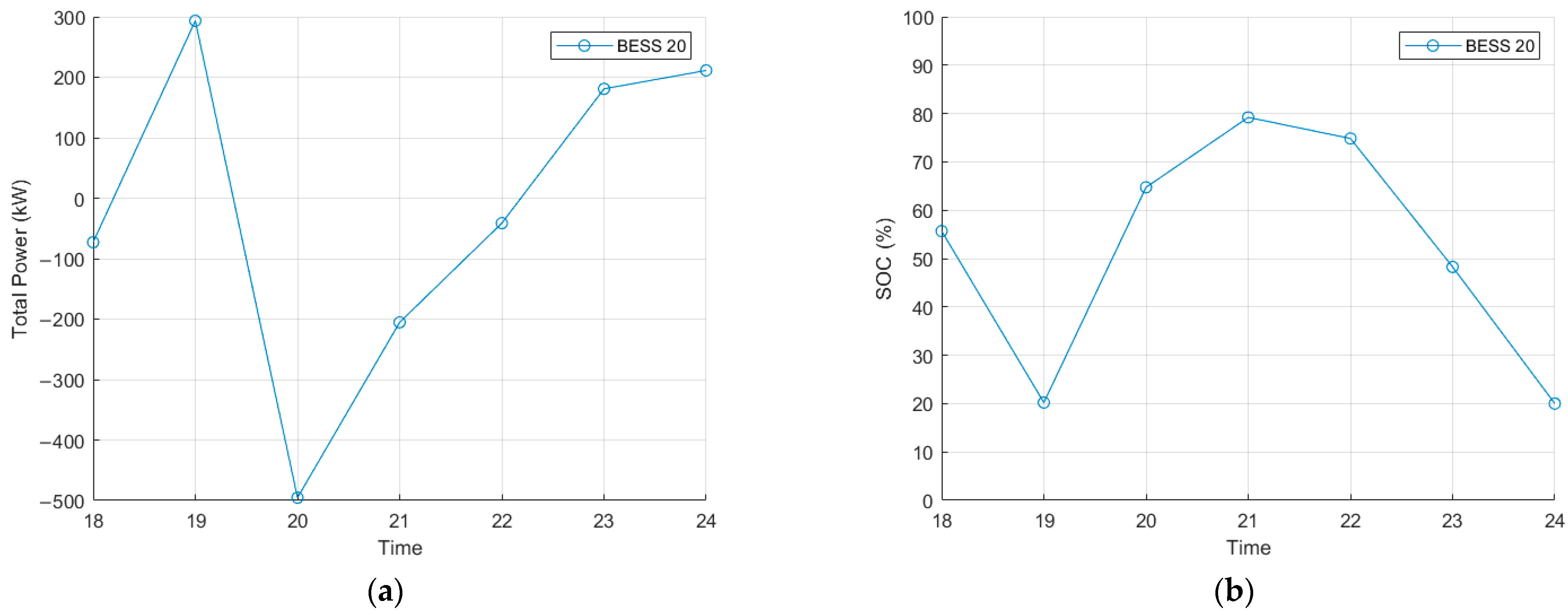
3.2.6. BESS Charging and Discharging Constraints
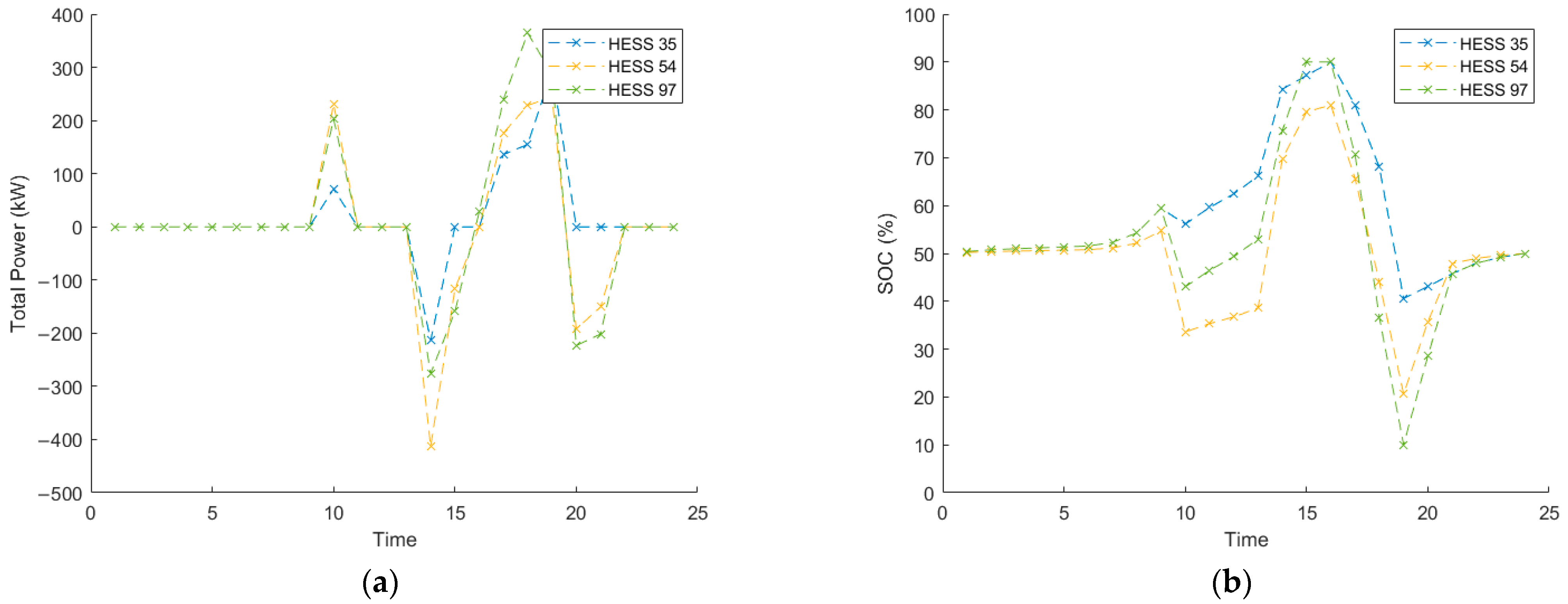
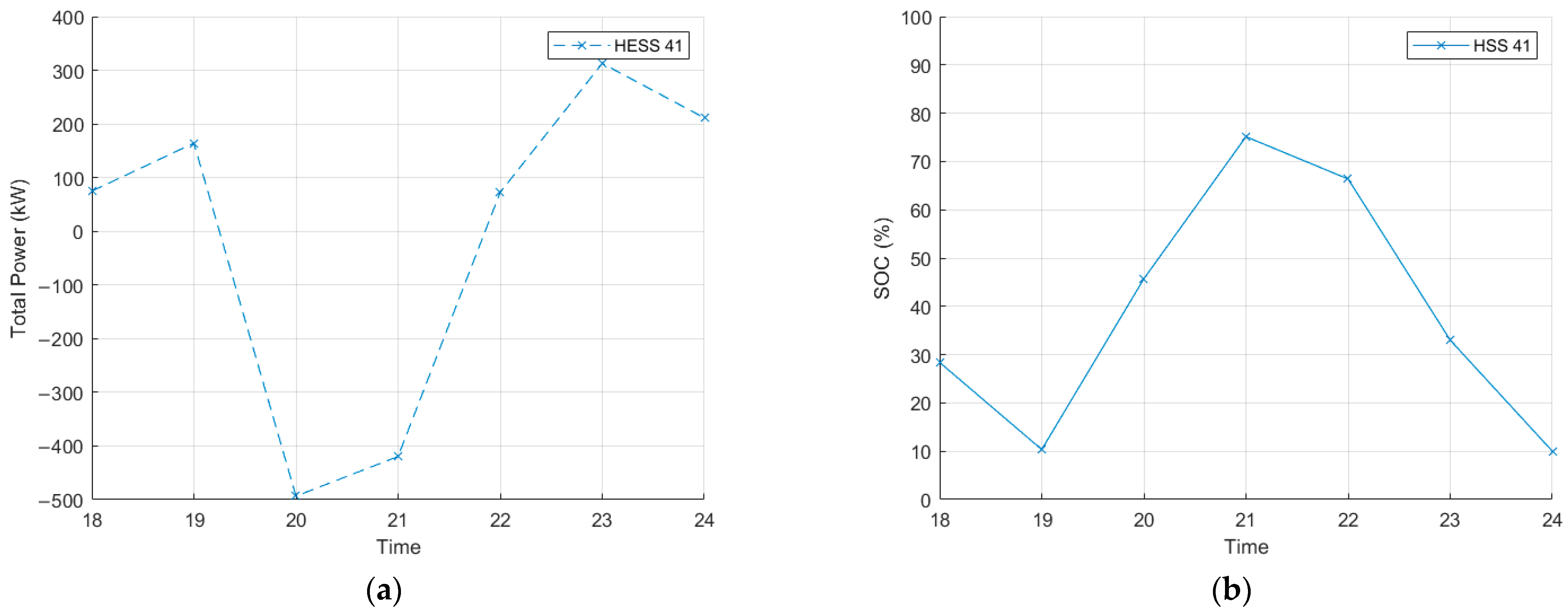
3.2.7. HESS Charging and Discharging Constraints
3.3. Microgrid Optimal Rescheduling After Fault by Disaster
3.3.1. Fault Scenarios and Power Management
3.3.2. Reconstruction of the Objective Function and Constraints
3.4. Electric Pricing for Key Customers
3.4.1. Outage Compensation Cost
3.4.2. Penalty Based on Voltage Sensitivity
3.4.3. Total Electricity Contract Price
4. Result Analysis
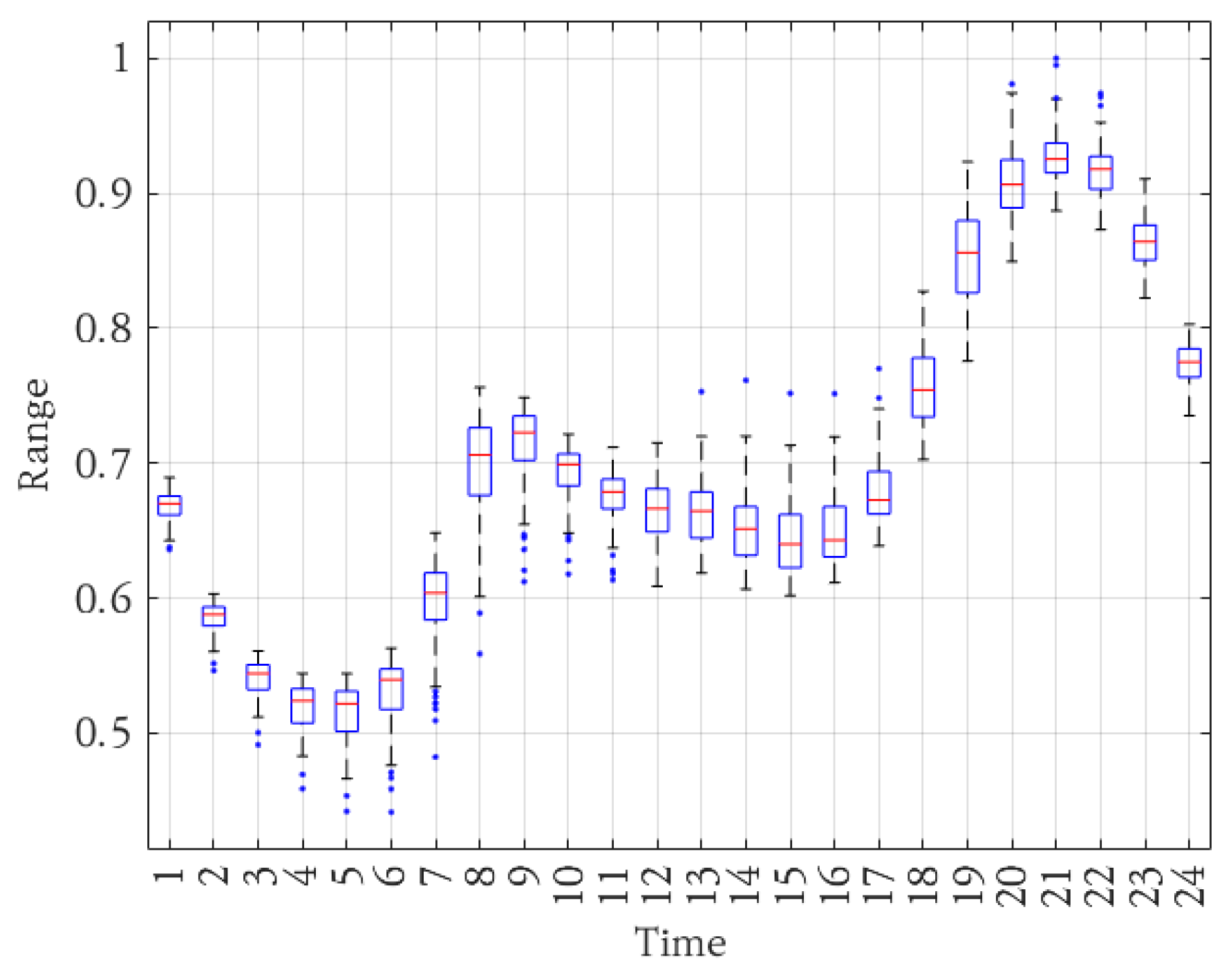
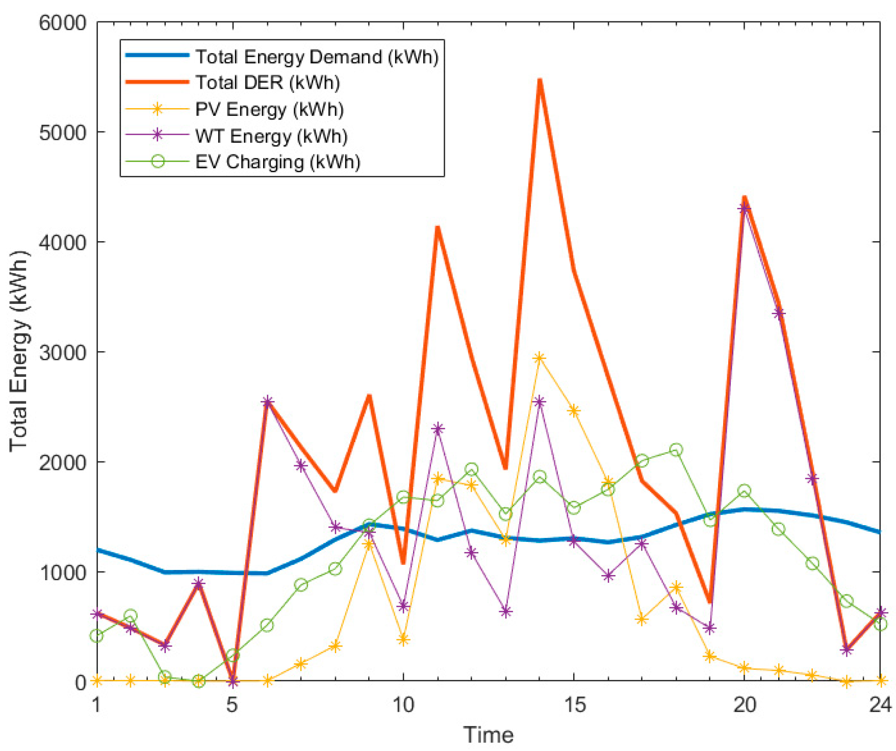
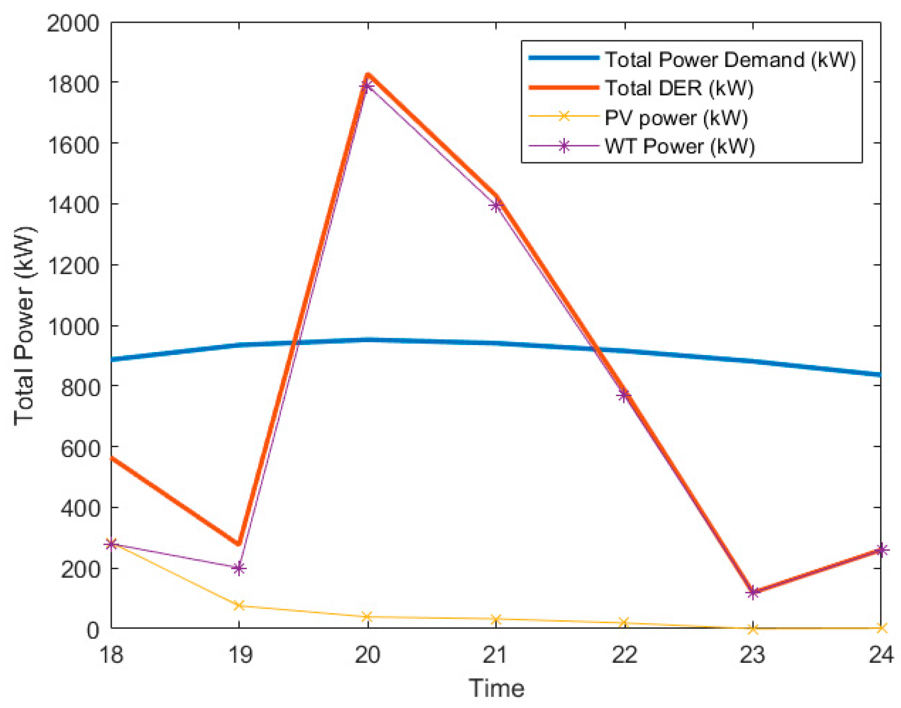
4.1. Load and RES Profiles
4.2. Parameter Settings
4.3. Data Preprocessing
4.4. Simulation Results and Analysis
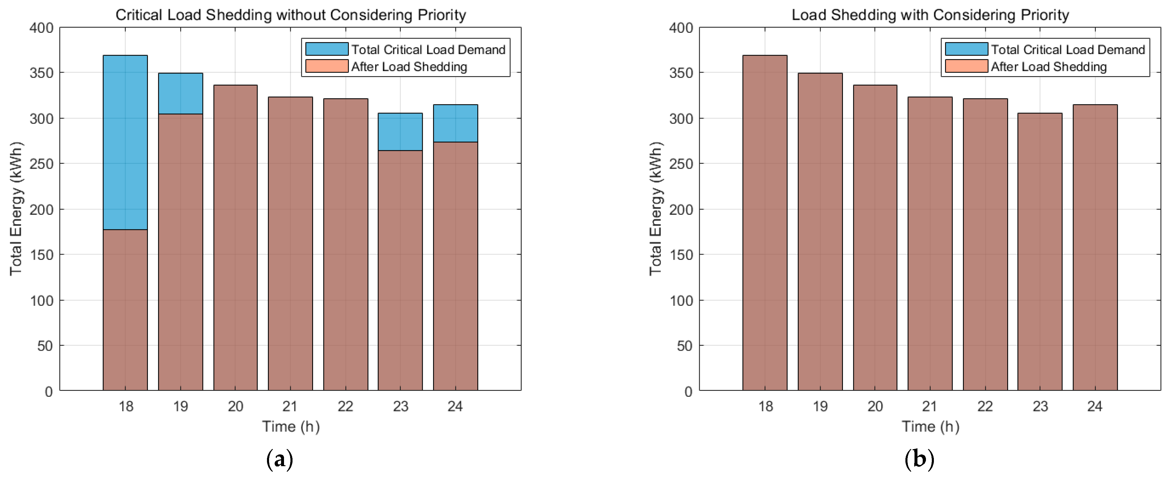
4.4.1. Estimating Outage Compensation Cost Based on Optimal Scheduling
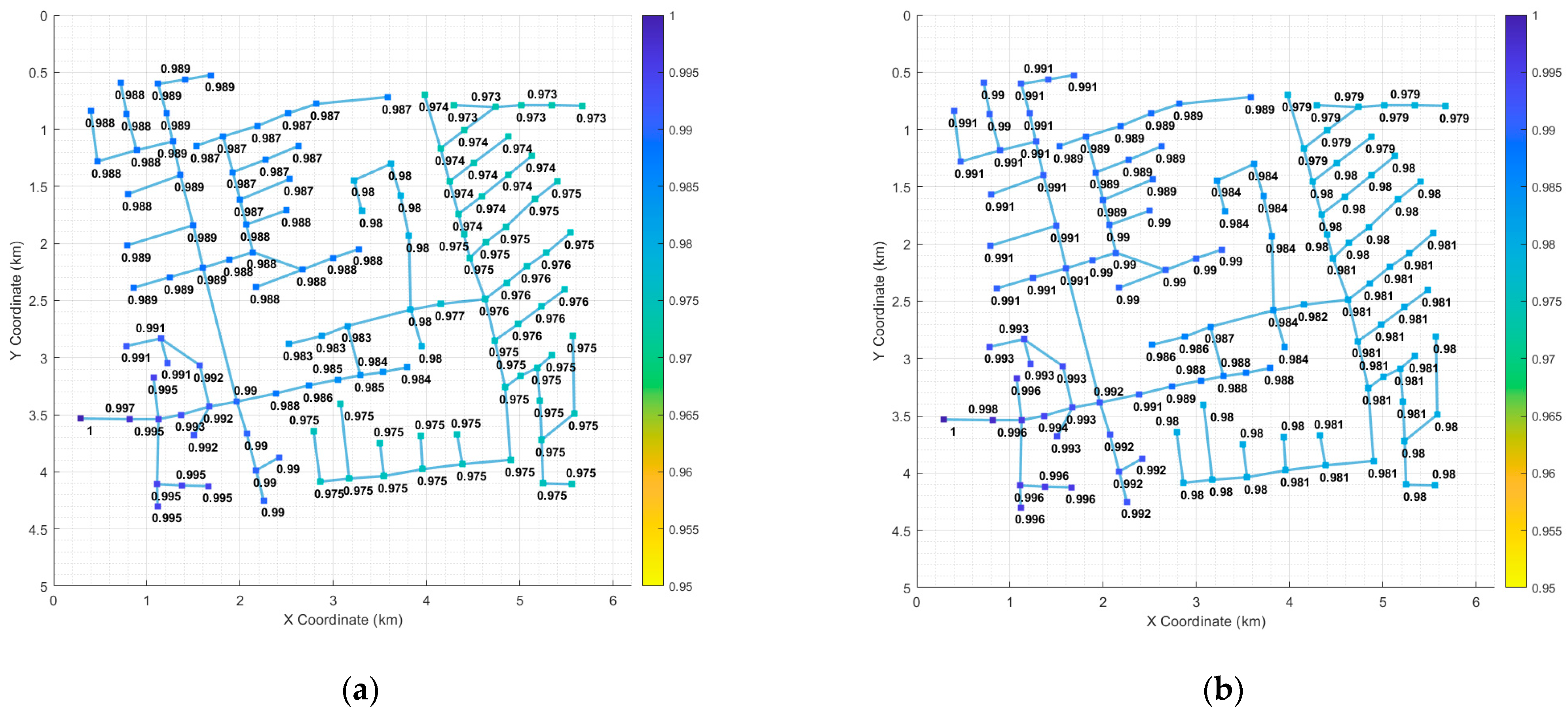
4.4.2. Estimating Voltage Stability Penalty Based on Voltage Variation
4.4.3. Estimating Electricity Price Based on Compensation Cost and Voltage Variation
4.5. Discussion
5. Conclusions
Author Contributions
Funding
Institutional Review Board Statement
Informed Consent Statement
Data Availability Statement
Conflicts of Interest
Abbreviations
| DER | Distributed energy resource |
| EV | Electric vehicle |
| FCEV | Fuel cell electric vehicle |
| PV | Photovoltaic |
| WT | Wind turbine |
| BESS | Battery energy storage system |
| HESS | Hydrogen energy storage system |
| SOCP | Second-order conic programming |
| MISOCP | Mixed-integer second-order conic programming |
| ESS | Energy storage system |
| HILP | High impact, low probability |
| FERC | Federal Energy Regulatory Commission |
| MILP | Mixed-integer linear programming |
| SOC | State-of-charge |
| V2G | Vehicle-to-Grid |
| BMS | Battery management system |
| PCS | Power conversion system |
| BOP | Balance of Plant |
| O&M | Operation and maintenance |
| TOU | Time of use |
Appendix A

| Parameter | Meaning |
|---|---|
| The total operation cost of the microgrid | |
| The total cost of power trade with outer grid | |
| The total cost of RES | |
| The total cost of ESS maintenance | |
| The total cost of EV charging | |
| The total revenue of customer sales | |
| The costs of purchasing power from the outer grid at time | |
| The costs of selling power to the outer grid at time | |
| The quantities of power purchased from the outer grid at time | |
| The quantities of power sold to the outer grid at time | |
| The purchasing cost of RES power at time | |
| The quantities of RES power generated at time located on bus | |
| The maintenance costs of the BESS | |
| The maintenance costs of the HESS | |
| The charging quantities of the BESS on the bus at time | |
| The discharging quantities of the BESS on the bus at time | |
| The quantities of the HESS output on the bus at time | |
| The EV charging price at time | |
| The quantities of EV charging on the bus at time | |
| The selling price of the power company to customers at time | |
| The demand of the loads on the bus at time | |
| The total demand of key customers | |
| The total demand of residential customers | |
| The total demand of key and residential customers | |
| The total demand of data station | |
| The total demand of hospital | |
| The total demand of communication station | |
| The total power generated by PV | |
| The total power generated by WT | |
| The total power generated by RES | |
| The total power generated by BESS | |
| The total power generated by HESS | |
| The total demand of customer | |
| The total demand of EV | |
| The total demand of FCEV | |
| The ratio of reactive power to active power | |
| The reactive power supplied by RES | |
| The sum of charging/discharging of the BESS on the bus at time | |
| The maximum output of the BESS | |
| The rated energy capacity of the BESS | |
| The SOC of the BESS on the bus at time | |
| The minimum SOC of the BESS | |
| The maximum SOC of the BESS | |
| The initial SOC of the BESS | |
| The final SOC of the BESS | |
| The conversion efficiency during charging of the BESS | |
| The conversion efficiency during discharging of the BESS | |
| The power from the fuel cell of the HESS on the bus at time | |
| The hydrogen from the electrolyzer of the HESS on the bus at time | |
| The maximum output of the fuel cell | |
| The maximum output of the electrolyzer | |
| The hydrogen produced by the electrolyzer | |
| The hydrogen consumed by the fuel cell | |
| The maximum capacity of hydrogen tank | |
| The hydrogen demand of FCEV | |
| The SOC of the HESS on the bus at time | |
| The minimum SOC of the HESS | |
| The maximum SOC of the HESS | |
| The initial SOC of the HESS | |
| The final SOC of the HESS | |
| The conversion efficiencies from hydrogen to electricity | |
| The conversion efficiencies from electricity to hydrogen | |
| The total amount of power not supplied due to outages | |
| The switches for normal loads on the bus at time | |
| The switches for critical loads on the bus at time | |
| The weights assigned to normal loads on the bus | |
| The weights assigned to critical loads on the bus | |
| The demand of normal loads on the bus at time | |
| The demand of critical loads on the bus at time | |
| The power generated by PVs on the bus at time | |
| The power generated by WTs on the bus at time | |
| The combined output from the BESS and HESS on the bus at time | |
| The total compensation cost under the general supply scenario | |
| The total compensation cost under the prioritized supply scenario | |
| The unsupplied load demand on the bus at time | |
| The compensation cost of the outage | |
| The additional infrastructure expansion cost | |
| The cost incurred for installing new power infrastructure | |
| The system voltage at bus before the contracted load is connected | |
| The system voltage at bus when the contracted load is connected | |
| The final contract price for key customers | |
| , | The voltage of the bus or |
| The current of the line between and | |
| The resistance of the line between and | |
| The reactance of the line between and | |
| The active power flowing through the line between and | |
| The reactive power flowing through the line between and | |
| The active power at bus | |
| The reactive power at bus | |
| The minimum voltage | |
| The maximum voltage | |
| The maximum current | |
| The total active power of the grid | |
| The total reactive power of the grid | |
| Time variable | |
| Time scale | |
| Bus number | |
| The total number of buses in the network | |
| The set of buses in the isolated network | |
| The set of time intervals following the outage |
References
- Stephanie, P. Federal Regulation for a “Resilient” Electricity Grid. Ecol. Law Q. 2019, 46, 417. [Google Scholar] [CrossRef]
- Sun, X.; Chen, J.; Zhao, H.; Zhang, W.; Zhang, Y. Sequential Disaster Recovery Strategy for Resilient Distribution Network Based on Cyber–Physical Collaborative Optimization. IEEE Trans. Smart Grid 2023, 14, 1173. [Google Scholar] [CrossRef]
- Qi, M.; Zhang, F.; Zhang, G. Sequential disaster recovery strategy for distribution network considering maintenance crew scheduling. J. Phys. 2024, 2823, 012062. [Google Scholar] [CrossRef]
- Liu, W.; Xu, Q.; Qin, M.; Yang, Y. A Post-Disaster Fault Recovery Model for Distribution Networks Considering Road Damage and Dual Repair Teams. Energies 2024, 17, 5020. [Google Scholar] [CrossRef]
- Moglen, R.; Leibowicz, B.D.; Kwasinski, A.; Cruse, G. Optimal restoration of power infrastructure following a disaster with environmental hazards. Socio-Econ. Plan. Sci. 2024, 95, 101974. [Google Scholar] [CrossRef]
- Zhang, X.; Son, Y.; Choi, S. Optimal scheduling of battery energy storage systems and demand response for distribution systems with high penetration of renewable energy sources. Energies 2022, 15, 2212. [Google Scholar] [CrossRef]
- Zhang, X.; Son, Y.; Cheong, T.; Choi, S. Affine-arithmetic-based microgrid interval optimization considering uncertainty and battery energy storage system degradation. Energy 2022, 242, 123015. [Google Scholar] [CrossRef]
- Zhang, X.; Woo, H.; Choi, S. An interval power flow method for radial distribution systems based on hybrid second-order cone and linear programming. Sustain. Energy Grids Netw. 2023, 36, 101158. [Google Scholar] [CrossRef]
- Zhang, X.; Shin, D.; Son, Y.; Woo, H.; Kim, S.-Y.; Choi, S. Three-stage flexibility provision framework for radial distribution systems considering uncertainties. IEEE Trans. Sustain. Energy 2023, 14, 948. [Google Scholar] [CrossRef]
- Balasubramaniam, K.; Saraf, P.; Hadidi, R.; Makaram, E.B. Energy management system for enhanced resiliency of microgrids during islanded operation. Electr. Power Syst. Res 2016, 137, 133. [Google Scholar] [CrossRef]
- Zafar, R.; Mahmood, A.; Razzaq, S.; Ali, W.; Naeem, U.; Shehzad, K. Prosumer based energy management and sharing in smart grid. Renew. Sustain. Energy Rev. 2018, 82, 1675. [Google Scholar] [CrossRef]
- Gao, H.; Chen, Y.; Xu, Y.; Liu, C.-C. Resilience-Oriented Critical Load Restoration Using Microgrids in Distribution Systems. IEEE Trans. Smart Grid 2016, 7, 2837. [Google Scholar] [CrossRef]
- Rajbhandari, Y.; Marahatta, A.; Shrestha, A.; Gachhadar, A.; Thapa, A.; Gonzalez-Longatt, F.; Guerrero, J.M.; Korba, P. Load prioritization technique to guarantee the continuous electric supply for essential loads in rural microgrids. Int. J. Elec. Power 2022, 134, 107398. [Google Scholar] [CrossRef]
- Tostado-Véliz, M.; Jordehi, A.R.; Fernández-Lobato, L.; Jurado, F. Robust energy management in isolated microgrids with hydrogen storage and demand response. Appl. Energy 2023, 345, 121319. [Google Scholar] [CrossRef]
- Su, J.; Zhang, R.; Dehghanian, P.; Kapourchali, M.H.; Choi, S.; Ding, Z. Renewable-dominated mobility-as-a-service framework for resilience delivery in hydrogen-accommodated microgrids. Int. J. Electr. Power Energy Syst. 2024, 159, 110047. [Google Scholar] [CrossRef]
- Yoon, Y.; Son, Y.; Choi, S. Deep reinforcement learning-based operation strategy for high resilience distribution system. IET Conference Proceedings. IET Conf. Proc. 2025, 2024, 1132. [Google Scholar] [CrossRef]
- Hosseini, M.M.; Parvania, M. Resilient Operation of Distribution Grids Using Deep Reinforcement Learning. IEEE Trans. Ind. Inform. 2022, 18, 2100. [Google Scholar] [CrossRef]
- Gautam, M.; Abdelmalak, M.; MansourLakouraj, M.; Benidris, M.; Livani, H. Reconfiguration of Distribution Networks for Resilience Enhancement: A Deep Reinforcement Learning-based Approach. In Proceedings of the IEEE IAS, Detroit, MI, USA, 9–14 October 2022; p. 1. [Google Scholar] [CrossRef]
- Sharifpour, M.; Ameli, M.T.; Ameli, H.; Strbac, G. A Resilience-Oriented Approach for Microgrid Energy Management with Hydrogen Integration during Extreme Events. Energies 2023, 16, 8099. [Google Scholar] [CrossRef]
- Garcia-Torres, F.; Valverde, L.; Bordons, C. Optimal Load Sharing of Hydrogen-Based Microgrids With Hybrid Storage Using Model-Predictive Control. IEEE Trans. Ind. Electron. 2016, 63, 4919. [Google Scholar] [CrossRef]
- Son, Y.; Woo, H.; Noh, J.; Dehghanian, P.; Zhang, X.; Choi, S. Optimization of energy storage scheduling considering variable-type minimum SOC for enhanced disaster preparedness. J. Energy Storage 2024, 93, 112366. [Google Scholar] [CrossRef]
- Correia, A.F.M.; Antonio Goncalves Neves, M.; Isabel Casal Dos Reis, A.; Paulo Coimbra, A.; Richard de Oliveira de Almeida, T.; Moura, P.; de Almeida, A.T. Architecture and Operational Control for Resilient Microgrids—A University Case Study. IEEE Access 2025, 13, 51373. [Google Scholar] [CrossRef]
- Correia, A.F.M.; Moura, P.; de Almeida, A.T. Technical and Economic Assessment of Battery Storage and Vehicle-to-Grid Systems in Building Microgrids. Energies 2022, 15, 8905. [Google Scholar] [CrossRef]
- Masoud, F.; Steven, H.L. Branch Flow Model: Relaxations and Convexification-Part I. IEEE Trans. Power Syst. 2013, 28, 2554. [Google Scholar] [CrossRef]
- Woo, H.; Son, Y.; Cho, J.; Choi, S. Stochastic second-order conic programming for optimal sizing of distributed generator units and electric vehicle charging stations. Sustainability 2022, 14, 4964. [Google Scholar] [CrossRef]
- Qin, j.; Wan, Y.; Li, F.; Kang, Y.; Fu, W. Distributed Economic Operation in Smart Grid: Model-Based and Model-Free Perspectives, 1st ed.; Springer Nature: Singapore, 2023; p. 455. [Google Scholar] [CrossRef]
| Parameter | Value |
|---|---|
| Minimum voltage | 0.9 p.u. |
| Maximum voltage | 1.1 p.u. |
| Maximum current | 11.24 p.u. |
| Power factor of RES | 0.95 |
| Capacity of BESS | 500 kWh |
| Maximum power of BESS | 300 kW |
| Maximum SOC of BESS | 90% |
| Efficiency of Charge/Discharge | 90% |
| Initial SOC of BESS | 50% |
| Final SOC of BESS | 50% |
| Capacity of HESS | 25 kg |
| Maximum SOC of HESS | 90% |
| Minimum SOC of HESS | 10% |
| Initial SOC of HESS | 50% |
| Final SOC of HESS | 50% |
| Maximum power of Fuel Cell | 200 kW |
| Maximum Power of Electrolyzer | 200 kW |
| Ratio of Hydrogen to Power | 40 kWh/kg |
| Ratio of Power to Hydrogen | 0.018 kg/kWh |
| Parameter | Value |
|---|---|
| Total Load Demand | 6345.08 kWh |
| Total Available Resources | 5694.28 kWh |
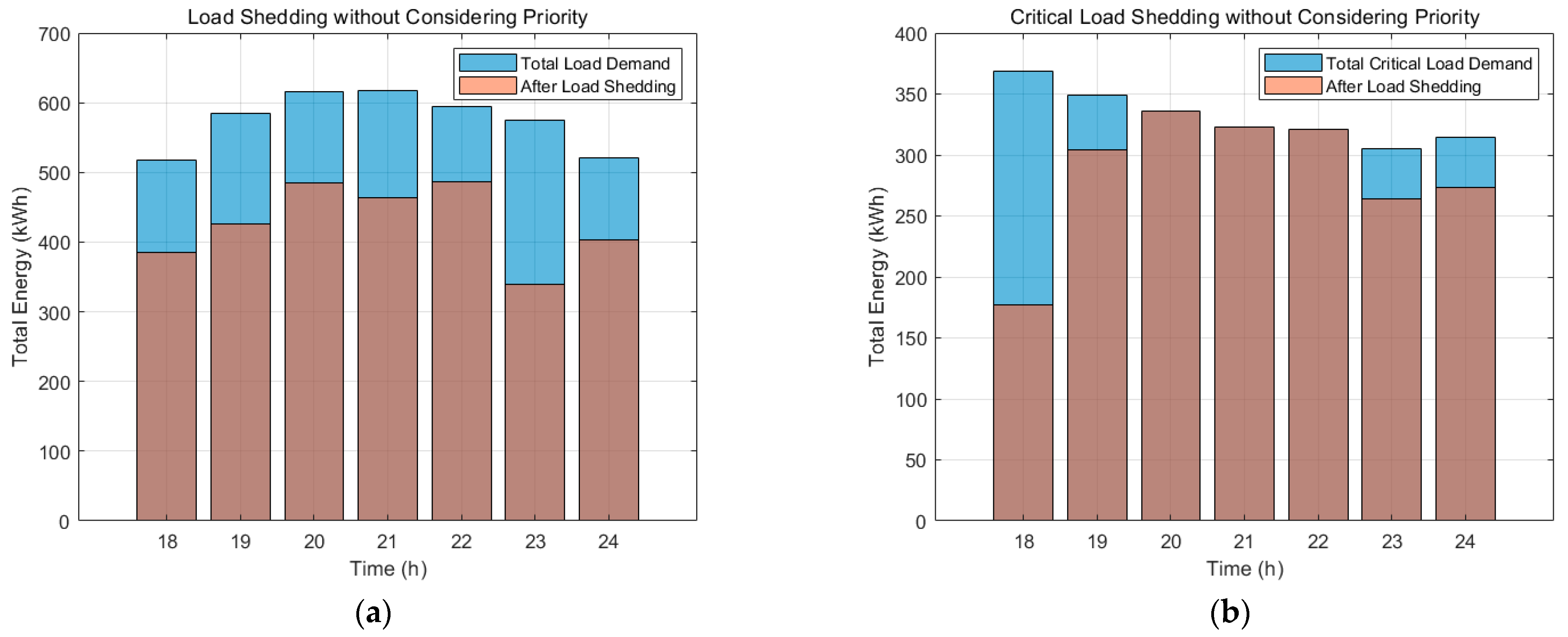
| Total Load | After Shedding (Normal Load) | After Shedding (Critical Load) | |
|---|---|---|---|
| No Priority | 4029.07 kWh | 2988.51 kWh | 1997.06 kWh |
| Key Customer Priority | 2775.99 kWh | 2316.28 kWh |
| Base Case | Data Center Case | |
|---|---|---|
| Average Voltage | 0.989 p.u. | 0.986 p.u. |
| Max Voltage | 1.000 p.u. | 1.000 p.u. |
| Min Voltage | 0.982 p.u. | 0.979 p.u. |
| Parameters | Value |
|---|---|
| Unsupplied Normal Load | 212.52 kWh |
| Weight Range | ×3 (7 h, Segment 2) |
| Maximum TOU Price | 0.2308 $/kWh |
| Compensation Cost | $147.15 |
| Parameters | Cost |
|---|---|
| Installation Cost (D/L) | $150,000 per km |
| O&M Cost | $3000 per year |
| Voltage Drop Penalty | 3% |
| Investment Cost | $4590 per year |
| Parameters | Base Case | Priority Supply Case |
|---|---|---|
| Compensation Cost | - | $147.15 |
| Investment Cost | - | $4590 |
| Final Contract Price | $0.0862~0.2308 | $0.6270~0.7715 |
Disclaimer/Publisher’s Note: The statements, opinions and data contained in all publications are solely those of the individual author(s) and contributor(s) and not of MDPI and/or the editor(s). MDPI and/or the editor(s) disclaim responsibility for any injury to people or property resulting from any ideas, methods, instructions or products referred to in the content. |
© 2025 by the authors. Licensee MDPI, Basel, Switzerland. This article is an open access article distributed under the terms and conditions of the Creative Commons Attribution (CC BY) license (https://creativecommons.org/licenses/by/4.0/).
Share and Cite
Kim, S.; Son, Y.; Woo, H.; Zhang, X.; Choi, S. A Pricing Strategy for Key Customers: A Method Considering Disaster Outage Compensation and System Stability Penalty. Sustainability 2025, 17, 4506. https://doi.org/10.3390/su17104506
Kim S, Son Y, Woo H, Zhang X, Choi S. A Pricing Strategy for Key Customers: A Method Considering Disaster Outage Compensation and System Stability Penalty. Sustainability. 2025; 17(10):4506. https://doi.org/10.3390/su17104506
Chicago/Turabian StyleKim, Seonghyeon, Yongju Son, Hyeon Woo, Xuehan Zhang, and Sungyun Choi. 2025. "A Pricing Strategy for Key Customers: A Method Considering Disaster Outage Compensation and System Stability Penalty" Sustainability 17, no. 10: 4506. https://doi.org/10.3390/su17104506
APA StyleKim, S., Son, Y., Woo, H., Zhang, X., & Choi, S. (2025). A Pricing Strategy for Key Customers: A Method Considering Disaster Outage Compensation and System Stability Penalty. Sustainability, 17(10), 4506. https://doi.org/10.3390/su17104506