A Study on the Speed Decision Control of Agricultural Vehicles in a Collaborative Multi-Machine Operation Scenario

Abstract

The driving speed of autonomous agricultural vehicles is influenced by surrounding cooperative vehicles during cooperative operations, leading to challenges in simultaneously optimizing operational efficiency, energy consumption, safety, and driving smoothness. This bottleneck hinders the development of autonomous cooperative systems. To address this, we propose a hierarchical speed decision control framework. The speed decision layer employs a maximum entropy-constrained proximal policy optimization (DMEPPO) reinforcement learning method, incorporating operational efficiency, energy consumption, safety, and smoothness as reward metrics to determine the optimal speed target. The speed control layer utilizes a Linear Matrix Inequality (LMI)-based robust control method for precise speed tracking. The experimental results demonstrate that the proposed DMEPPO achieved convergence after 2000 iterations and better learning performance, while the LMI-based controller achieved robust and responsive tracking. This architecture provides a theoretical foundation for speed decision control in agricultural vehicle cooperation scenarios. By considering aspects of speed decision-making control such as energy conservation, good solutions can be provided for the sustainable development of agriculture.

1. Introduction

The speed control problem is the first problem that needs to be solved regarding autonomous driving in agricultural vehicle cooperation scenarios. In the process of developing speed control, it is essential to holistically take into account various control goals, including operational effectiveness, low energy usage, safety, and driving smoothness.

Speed control is widely considered in the vehicle domain. Model-based control methods are adopted most often, providing good control synthesis [1]. Zhao S et al. proposed a multi-objective control method for following vehicles based on explicit model predictive control (EMPC) theory by designing a search process involving an online lookup table by locating the partition at which the current state was located and then applying this explicit control law to achieve speed control [2]; then, a stochastic MPC method was proposed to optimize the fuel consumption of the vehicle in the vehicle speed tracking environment by using the speed of the preceding vehicle for short-term prediction to solve the constrained motion level optimal control problem [3].

To make speed control applicable to real-time situations, studies [4,5,6,7,8] have established a speed control model based on empirical measurements of computer-driven vehicles in the real environment and realized speed tracking control by means of relevant control algorithms. However, this method requires the accumulation of a priori data measurements. Wang C et al. proposed the idea of dynamically optimizing the idealized fixed information flow topologies (IFTs) to improve the data stability and improve the speed tracking performance [9]. Li T et al. proposed an MPC speed tracking controller with an adaptive compensation capability based on a Kalman filter to realize speed control [10].

However, the complex field operation environment results in a lack of adaptability in speed control for agricultural vehicles. To improve the control accuracy, an electro-hydraulic automatic mechanical gearshift device, as well as an automatic throttle adjustment device, was developed to realize fixed-speed control using a proportion–integration–differentiation (PID) control algorithm [11]. Then, an autonomous following vehicle test platform was built, which could achieve a small following error [12,13]. As traditional longitudinal control algorithms rely on accurate vehicle dynamic modeling or complex controller parameter calibrations, a longitudinal control algorithm based on Radial Basis Function (RBF)-PID has been proposed to achieve vehicle speed control with a self-tuning capability [14]. In order to improve the speed tracking performance of a direct rice seeding machine operating in harsh environments such as paddy fields, Mehraban, Z. et al. proposed a fuzzy adaptive cruise control method by integrating fuzzy control with MPC to enhance both the longitudinal safety and fuel efficiency by considering the real-time conditions [15]. Yin X. et al. carried out an autopilot speed control study with an upland gap plant protection machine with good results [16]. Wu Z. et al. studied a drive torque model under cruise operation conditions [17].

To enhance the precision of speed control, the Linear Quadratic Regulator (LQR) technique has been utilized [18]. To improve stability and robustness, an MPC-based speed tracking method was proposed [19]. In order to solve the speed control constraint problem, a continuous-time primal–dual algorithm for tracking the speed was proposed [20]. However, it is difficult to meet the multi-objective speed requirement effectively even with robust pure speed control. He X et al. proposed a multi-objective speed decision-making method based on entropy-constrained proximal policy optimization (ECPPO) [21], but it could not cope with a speed control problem involving uncertainties and disturbances in a dynamic environment.

For unmanned agricultural vehicle speed control, determining how to achieve unmanned agricultural vehicle multi-objective dynamic speed control in a dynamic environment is very important. It is necessary to comprehensively consider the performance requirements of high operational efficiency, low agricultural vehicle energy consumption, smoothness, and safety at the same time. Furthermore, it is also necessary to be able to cope with the various types of uncertainty and interference brought about by the complex field operating environment, so as to effectively resist uncertainties and disturbances while meeting the requirement of realizing multiple objectives in a dynamic environment for the speed control system of an unmanned agricultural vehicle.

This study introduces a robust, optimal speed control approach for unmanned agricultural vehicles, which integrates deep reinforcement learning (DRL) with robust control through a layered framework including a speed decision-making layer and speed control layer. In the speed decision-making layer, in order to make a decision on the optimal speed in a dynamic environment, a deep maximum entropy-constrained proximal policy optimization reinforcement learning algorithm (DMEPPO) based on dynamic environment information and heuristic goal entropy and adaptive entropy constraints is used. The speed control layer is designed to effectively track the learned optimal speed while simultaneously resisting uncertainties and disturbances, leveraging linear matrix inequalities (LMIs) to ensure robust speed controller performance for enhanced stability and precision in dynamic environments.

The points of innovation in this study can be summarized by the following two achievements: (1) Based on the collaborative operation scenario, a theoretical method for speed decision-making considering information on the surrounding agricultural vehicles is proposed, taking into account multiple speed control goals such as high operation efficiency, low energy consumption, safety, and smoothness and ultimately achieving optimal speed decision-making in a dynamic environment. (2) A speed decision control architecture combining reinforcement learning and robust control is proposed. After determining the optimal speed target through reinforcement learning, speed tracking control is carried out using a robust control method to achieve the precise speed control of multiple targets.

The hierarchical speed decision control framework (DMEPPO + LMI) proposed in this study not only solves the technical challenge of multi-objective dynamic optimization but also provides a practical solution for the sustainable development of agriculture. First, through the integrated optimization of the operation efficiency and energy consumption using a deep reinforcement learning algorithm (DMEPPO), the system is able to autonomously select the optimal speed target in a dynamic environment, which significantly reduces fuel consumption (e.g., simulation experiments showed that the energy consumption was reduced by about 30%) and thus reduces the carbon emissions and operation costs. Secondly, the robust control layer (LMI) ensures the smoothness of the vehicle’s driving by suppressing the uncertainty of disturbances in the complex environment of a field, prolonging the service life of mechanical parts, and reducing the wear and tear of equipment and the need for maintenance due to frequent acceleration or braking. In addition, the introduction of the safety distance reward mechanism effectively avoids the risk of collision in multi-machine cooperation, improves operational safety, and further ensures the high efficiency and resource-saving capability of agricultural production. These innovative designs not only meet the demand for intelligence and precision in modern agriculture but also provide technical support for the development of low-carbon and green agriculture, which is in line with the strategic goal of the sustainable development of global agriculture.

This paper is organized as follows. The preliminaries are discussed in Section 1. Speed control modeling for driverless agricultural vehicles is shown in Section 2. The speed decision-making and control design is shown in Section 3. The experimental method is described in Section 4. The results and discussion are included in Section 5.

2. Preliminaries

2.1. Constrained Markov Decision-Making (CMDP)

This paper views the continuous state and action transitions of a driverless agricultural vehicle as Markov decision processes (MDPs). Its state–action transitions take into account additional entropy constraints and are often referred to as Constrained Markov Decision Processes (CMDPs). A CMDP can be described as a tuple, (S, A, R, P, C, d), where S represents the set of all states in which the intelligent body engages in interaction with the setting, A is the set of possible actions the intelligent body can take, R stands for the incentive function, P is the state transfer probability function from the current state to the next state, C is the cost function, and d is a set of constraints limiting the generalization of multiple constraints [22].

2.2. Actor–Critic Architecture (AC)

The Actor–Critic architecture consists of the Actor model and the Critic model, commonly used in DRL. The Critic model serves as an evaluative component, calculating the state value function (V(s)) to represent the expected cumulative reward in each state (s) and the action value function (Q(a|s)) to quantify the expected reward of taking action (a) in a given state (s). The Critic evaluates actions by comparing their predicted outcomes, providing a basis for decision-making. Meanwhile, the Actor model generates actions based on its current policy, and the Actor model is updated according to the direction suggested by the Critic model [23].

2.3. Policy Gradient (PG)

The PG algorithm is a reinforcement learning (RL) algorithm [24]. The PG algorithm focuses on optimizing the expected value of the cumulative reward, which is the objective of this paper. A gradient descent is usually used to update the parameter θ, which can be expressed as

$$\overline{R}=E_t[{\nabla }_{\theta }\log {\pi }_{\theta }(a_t|s_t){\widehat{A}}_t]$$

(1)

where E_t denotes the expectation for a set of samples, π_θ is a randomized strategy based on the parameter θ, and ${\widehat{A}}_t$ is the dominance function, which can be expressed as

$${\widehat{A}}_t=Q_{{\pi }_{\theta }}(s_t,a_t)-V_{{\pi }_{\theta }}(s_t)$$

(2)

where $Q_{{\pi }_{\theta }}(s_t,a_t)$ denotes the action value function of executing action a under policy π_θ in state s_t, and $V_{{\pi }_{\theta }}(s_t)$ denotes the value function for a state, s_t.

For computational purposes, a loss function is characterized as follows:

$$L(\theta )=E_t(\log {\pi }_{\theta }(a_t|s_t)A_t).$$

(3)

2.4. Proximal Policy Optimization Algorithm (PPO)

PPO is an algorithm tailored for online strategies, commonly employed in environments with continuous action spaces. It encompasses two primary forms: PPO-Penalty and PPO-Clip. The PPO-Clip variant does not incorporate a KL divergence term in its objective function. It is distinguished by its approach to adjusting the objective function, which ensures that the new strategy aligns closely with the old strategy [25].

The PPO-Clip approach modifies the policy using the parameter θ:

$$\theta =\arg \underset{\theta }{\max }\underset{s,a~{\pi }_{{\theta }_{\mathrm{old}}}}{E}[L(s,a,{\theta }_{\mathrm{old}},\theta )]$$

(4)

Using r_t(θ) to represent the ratio of the old and new strategies,

$$r_t(\theta )={\displaystyle \frac{{\pi }_{\theta }(a|s)}{{\pi }_{{\theta }_{\mathrm{old}}}(a|s)}}$$

(5)

To achieve the aim, the loss function L(s, a, θ_old, θ) is set:

$$L(s,a,{\theta }_{\mathrm{old}},\theta )=\min (r_t(\theta ){\widehat{A}}_t,clip(r_t(\theta ),1-\epsilon ,1+\epsilon )A_t)$$

(6)

where ε is a (small) hyperparameter that guarantees that the gap between the new strategy and the old one will be small.

At the same time, in order to estimate the size of the variation between the new and old strategies, the dominance objective function is set to be

$$L_{{\widehat{A}}_t}=-{{\displaystyle {\sum }_{t=1}^T({\displaystyle {\sum }_{t^{\prime }>t}{\gamma }^{t^{\prime }-t}{\tau }_{t^{\prime }}-V_{{\pi }_{\theta }}}(s_t))}}^2$$

(7)

where γ denotes the discount factor and ${\tau }_{t^{\prime }}$ is the reward at moment t′.

3. Speed Control Modeling for Driverless Agricultural Vehicles

The motion of a driverless agricultural vehicle is not always longitudinal; it is a synthetic motion that includes longitudinal, lateral, and yaw motions. When the agricultural vehicle’s motion direction changes, the lateral and yaw motions affect the longitudinal motion. Therefore, the lateral and yaw motions should be considered in the longitudinal motion modeling process.

Referring to the literature [26], the velocity tracking model is established as follows:

$$\left\{\begin{array}{l}{\dot{v}}_y=a_{11}{v}_y+a_{12}\dot{\psi }+b_1{\delta }_f+d_1\hfill \\ \ddot{\psi }=a_{21}{v}_y+a_{22}\dot{\psi }+b_2{\delta }_f+d_2\hfill \\ {\dot{v}}_x=\dot{\psi }{v}_y+F_x/m+d_3\hfill \end{array}\right.$$

(8)

where F_x is the longitudinal force on the wheels; d₁, d₂, and d₃ are the output interferences with different degrees of freedom; v_x and v_y are the longitudinal velocity and lateral velocity, respectively; δ_f is the front wheel angle; $\ddot{\psi }$ is rate of change in the yaw rate; and m is the agricultural vehicle’s overall mass.

The model parameters in Equation (8) are

$$a_{11}=-{\displaystyle \frac{(C_f+C_r)}{m{v}_x}},a_{12}=-v_x-{\displaystyle \frac{(a{C}_f-b{C}_r)}{m{v}_x}},a_{21}={\displaystyle \frac{b{C}_r-a{C}_f}{I_z}}$$

$$a_{22}=-{\displaystyle \frac{a^2{C}_f+b^2{C}_r}{v_x{I}_z}},b_1={\displaystyle \frac{C_f}{m}},b_2={\displaystyle \frac{a{C}_f}{I_z}}$$

where C_f and C_r are the cornering stiffness of the front and rear tires and I_z is the agricultural vehicle’s z-axis moment of inertia.

It should be noted that a driverless agricultural vehicle may encounter an uneven road surface, change in the road surface adhesion coefficient, change in the vehicle mass, etc., when driving on the field road, and all these uncertainties will be shown in the tires’ lateral cornering stiffness, which in turn will affect the longitudinal and lateral control of the driverless agricultural vehicle [27]. Therefore, the uncertainty in the tires’ lateral cornering stiffness should be considered in the modeling process:

$$\left\{\begin{array}{c}{C}_f=C_{f0}+{\Delta }_{C_f}\\ C_r=C_{r0}+{\Delta }_{C_r}\end{array}\right.$$

(9)

where C_f0 are C_r0 are nominal values of the lateral cornering stiffness of the front and rear tires, respectively, and ΔC_f and ΔC_r are the uncertainty in the lateral cornering stiffness of the front and rear tires.

Define the velocity error as

e_v = v_xr − v_x

(10)

where v_xr and v_x are the desired speed and actual speed of driverless agricultural vehicles, respectively.

In order to realize speed tracking, v_xr, the speed error e_v should be minimized. Combining (8) and (10), the state space representation is obtained as

$$\left\{\begin{array}{l}{\dot{v}}_y=a_{11}{v}_y+a_{12}r+b_1{\delta }_f+d_1\hfill \\ \ddot{\psi }=a_{21}{v}_y+a_{22}r+b_2{\delta }_f+d_2\hfill \\ {\dot{e}}_v=r{v}_y+F_x/m-{\dot{v}}_{xr}+d_3\hfill \end{array}\right.$$

(11)

Defining the state variable as $x(t)={\left[\begin{array}{ccc}{v}_y& r& e_v\end{array}\right]}^{\mathrm{T}}$, the control inputs are $u(t)=F_x$. The external interference is $w(t)={\left[\begin{array}{ccc}{b}_1{\delta }_f+d_1& b_2{\delta }_f+d_2& -{\dot{v}}_{xr}+d_3\end{array}\right]}^{\mathrm{T}}$.

The velocity tracking model state space can be represented as

$$\dot{x}(t)=Ax(t)+Bu(t)+w(t)$$

(12)

where $A=\left[\begin{array}{ccc}{a}_{11}& a_{12}& 0\\ a_{21}& a_{22}& 0\\ r& 0& 0\end{array}\right]$ and $B=\left[\begin{array}{c}0\\ 0\\ 1/m\end{array}\right]$.

During the design of the robust feedback controller, the yaw velocity and speed error e_v were selected for designing the output feedback controller.

The equation for the output can be written as

$$y(t)=C_{1}x(t)$$

(13)

where $C_1={\left[\begin{array}{ccc}0& 1& 1\end{array}\right]}^{\mathrm{T}}$.

In order to ensure the unmanned agricultural vehicle has both accurate speed tracking and traversal steadiness, an evaluation equation is established to make the transverse angular velocity and speed deviation as low as possible. Considering that the unmanned agricultural vehicle is mostly traveling in a straight line, the transverse velocity is small. Its evaluation equation is defined as

$$z(t)=C_{2}x(t)$$

(14)

where $C_2={\left[\begin{array}{ccc}1& 1& 1\end{array}\right]}^{\mathrm{T}}$.

Synthesizing (12) to (14), the velocity control model can be re-expressed as a generalized state space of the form

$$\left\{\begin{array}{l}\dot{x}(t)=Ax(t)+Bu(t)+w(t)\hfill \\ y(t)=C_{1}x(t)\hfill \\ z(t)=C_{2}x(t)\hfill \end{array}\right.$$

(15)

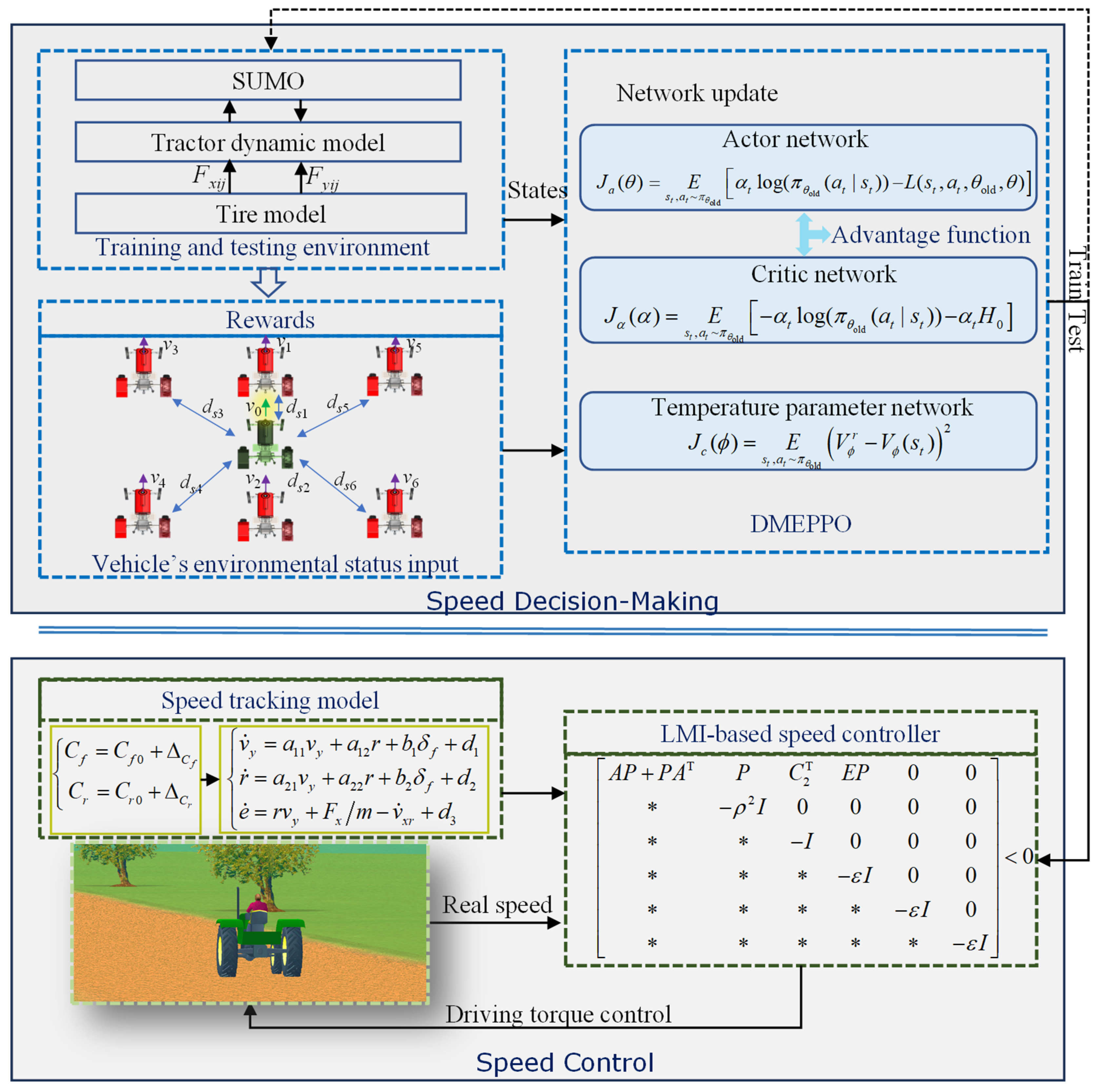
4. Speed Decision-Making and Control Design

4.1. Deep Maximization Entropy-Constrained Reinforcement Learning

Simple PPO tends to utilize a strategy to obtain higher rewards, resulting in the strategy being more likely to fall into a local optimum. The Actor–Critic theory serves as a key basis for incorporating entropy-increasing methods to enhance the exploratory randomness of strategies. Building on this, PPO can be adjusted to include a maximum entropy threshold, enabling the intelligent agent to escape local optima and discover more rewarding strategies. In addition, in order to enhance the learning efficiency, a target entropy constraint is set to ensure continuous adaptive adjustment with training [21].

The policy-constrained optimization problem in RL can be described as follows:

$$\begin{array}{l}\underset{{\pi }_0,\cdots {\pi }_T}{\max }E\left({\displaystyle {\sum }_{t=0}^{T}r(s_t,a_t)}\right)\\ s.t.\forall t{E}_{(s_t,a_t)~{\rho }_{\pi }}\left[-\log ({\pi }_t(a_t|s_t))\right]\ge H_0\end{array}$$

(16)

where ρ_π denotes the marginal state distribution’s actions under policy π_t(a_t|s_t). Let H₀ be the heuristic valuation of the strategy entropy. In order to enhance the exploration ability of the optimization-seeking strategy and achieve convergence as soon as possible, H₀ is set to decay adaptively with an increase in training, which can be expressed as

$$H_0={\varsigma }^t{H}_{fix}$$

(17)

where ς means the adaptive attenuation factor and H_fix means the initial entropy value.

Given that the reward at time t is independent of the previous action, dynamic programming can be applied to determine the highest expected reward for every possible strategy. Consequently, the aforementioned optimization goal (16) can be rephrased as

$$\underset{{\pi }_0}{\max }\left(E\left[r(s_0,a_0)\right]+\underset{{\pi }_1}{\max }\left(E[\cdots ]+\underset{{\pi }_T}{\max }E\left[r(s_T,a_T)\right]\right)\right)$$

(18)

It is then subjected to segmented objective optimization:

$$\begin{array}{l}\max E_{(s_T,a_T)~{\rho }_{\pi }}\left[r(s_T,a_T)\right]\\ s.t.H({\pi }_T)-H_0\ge 0\end{array}$$

(19)

where

$$H({\pi }_T)=E_{(s_T,a_T)~{\rho }_{\pi }}\left[-\log ({\pi }_T(a_T|s_T))\right]$$

(20)

Let $g({\pi }_T)=H({\pi }_T)-H_0$.

Combine (19) and (20) and perform the following equation definition:

$$f({\pi }_T)=\left\{\begin{array}{ll}{E}_{(s_T,a_T)~{\rho }_{\pi }}\left[r(s_T,a_T)\right]\hfill & ifh({\pi }_T)\ge 0\hfill \\ -\infty \hfill & else\hfill \end{array}\right.$$

(21)

Then, the constrained optimization problem can be expressed as

$$\max f({\pi }_T)s.t.h({\pi }_T)\ge 0$$

(22)

To address the constrained optimization issue in Equation (22), Lagrange multipliers are used for the temperature parameter ϑ to derive the following set of equations:

$$L({\pi }_T,{\vartheta }_T)=f({\pi }_T)+{\vartheta }_{T}h({\pi }_T)$$

(23)

The optimization problem with constraints constructed in this paper is solved by minimizing L(π_T, ϑ_T) using ϑ_T on the one hand and maximizing f(π_T) using π_T on the other hand. Consequently, we have the following equation:

$$\underset{{\pi }_T}{\max }f({\pi }_T)=\underset{{\pi }_T}{\max }\underset{{\vartheta }_T\ge 0}{\min }L({\pi }_T,{\vartheta }_T)$$

(24)

Equation (24) can be viewed as a dyadic function. According to the theory of a zero-sum game, through combining (21)–(24) we can obtain

$${\pi }_T^{*}=\arg \underset{{\pi }_T}{\max }{E}_{(s_T,{\vartheta }_T)~{\rho }_{\pi }}\left[r(s_T,a_T)+{\vartheta }_{T}g({\pi }_T)\right]$$

(25)

$${\vartheta }_T^{*}=\arg \underset{{\vartheta }_T\ge 0}{\min }{E}_{(s_T,{\vartheta }_T)~{\rho }_{{\pi }^{*}}}\left[{\vartheta }_{T}g({\pi }_T^{*})\right]$$

(26)

The subsequent execution steps perform the same iterative operations as the previous steps. In practical situations, the above formulas are difficult to solve directly. Considering that the use of a neural network has a good effect on the acquisition of training parameters, the above equation can be further solved as

$$\begin{array}{l}\underset{\theta }{\max }\underset{s_t,a_t~{\pi }_{{\theta }_{\mathrm{old}}}}{E}\left[L(s_t,a_t,{\theta }_{\mathrm{old}},\theta )\right]\\ s.t.\forall t,\underset{s_t,a_t~{\pi }_{{\theta }_{\mathrm{old}}}}{E}\left[-\log \left({\pi }_{{\theta }_{\mathrm{old}}}(a_t|s_t)\right)\right]\ge H_0\end{array}$$

(27)

where $t\in \left[0,T\right]$ and T is the sampling time.

According to the generalized dominance estimation method [28], the dominance function can be rewritten in the following form:

$${\widehat{A}}_t=V_{\varphi }^r-V_{\varphi }(s_t)+(\gamma \lambda )\left[V_{\varphi }^r-V_{\varphi }(s_t)\right]+\dots +{(\gamma \lambda )}^{T-t-1}\left[V_{\varphi }^r-V_{\varphi }(s_{T-1})\right]$$

(28)

$$V_{\varphi }^r=r_t+\gamma V_{\varphi }(s_{t+1})-{\alpha }_t\log \left({\pi }_{{\theta }_{\mathrm{old}}}(a_t|s_t)\right)$$

(29)

In this case, V_ϕ denotes the corresponding value function for ϕ.

Ultimately, the loss function for the action model is derived to be

$$J_a(\theta )=\underset{s_t,a_t~{\pi }_{{\theta }_{\mathrm{old}}}}{E}\left[{\alpha }_t\log ({\pi }_{{\theta }_{\mathrm{old}}}(a_t|s_t))-L(s_t,a_t,{\theta }_{\mathrm{old}},\theta )\right]$$

(30)

The temperature parameter ϑ can be obtained by training a network that minimizes the following loss function:

$$J_{\vartheta }(\vartheta )=\underset{s_t,a_t~{\pi }_{{\theta }_{\mathrm{old}}}}{E}\left[-{\vartheta }_t\log ({\pi }_{{\theta }_{\mathrm{old}}}(a_t|s_t))-{\vartheta }_t{H}_0\right]$$

(31)

The loss function of the evaluation model is

$$J_c(\varphi )=\underset{s_t,a_t~{\pi }_{{\theta }_{\mathrm{old}}}}{E}{\left(V_{\varphi }^r-V_{\varphi }(s_t)\right)}^2$$

(32)

The DMEPPO algorithm pseudocode is shown in Algorithm 1.

Algorithm 1. DMEPPO pseudocodes.

Input: Environment ε; Heuristic target entropy threshold H0

Initialize: Parameters θ, ϕ, ϑ

for $i\in \left\{1,\cdots ,N\right\}$ do

Run the strategy T times and collect $\left\{s_t,a_t,r_t,s_{t+1}\right\}$

Estimating the dominant function:

${\widehat{A}}_t={\displaystyle {\sum }_{t^{\prime }>t}{\gamma }^{t^{\prime }-t}}{\tau }_{t^{\prime }}-V_{{\pi }_{\theta }}(s_t)$

${\pi }_{\mathrm{old}}\leftarrow {\pi }_{\theta }$

for $j\in \left\{1,\cdots ,M\right\}$ do

$J_a(\theta )=\underset{s_t,a_t~{\pi }_{{\theta }_{\mathrm{old}}}}{E}\left[{\alpha }_t\log ({\pi }_{{\theta }_{\mathrm{old}}}(a_t|s_t))\right.\left.-L(s_t,a_t,{\theta }_{\mathrm{old}},\theta )\right]$

$J_{\vartheta }(\vartheta )=\underset{s_t,a_t~{\pi }_{{\theta }_{\mathrm{old}}}}{E}\left[-{\vartheta }_t\log ({\pi }_{{\theta }_{\mathrm{old}}}(a_t|s_t))\right.\left.-{\vartheta }_t{H}_0\right]$

$J_c(\varphi )=\underset{s_t,a_t~{\pi }_{{\theta }_{\mathrm{old}}}}{E}{\left(V_{\varphi }^r-V_{\varphi }(s_t)\right)}^2$

Updating parameters with gradient descent θ, ϕ, ϑ

end for

end for

4.2. Multi-Target Speed Rewards and Network Settings

The determination of the driving speed of driverless agricultural vehicles should consider multiple factors such as operational efficiency, fuel economy, safety, and the smoothness of driving in dynamic environments. Hence, crafting a proper reward function is crucial for achieving an optimal holistic outcome.

4.2.1. Consider the Rewards of Operational Efficiency

There is a certain positive correlation between operational efficiency and the speed of a driverless agricultural vehicle. Agricultural vehicles have an optimal operating speed range. Within the optimal operating range, the reward first increases and then decreases with the operating speed. When the speed is lower than the optimal speed, the reward increases with an increase in the operation speed. When the speed is higher than that of the optimal speed, the reward decreases as the speed increases. Also consider the fact that the speed change should be as smooth as possible to ensure good operational efficiency. Combining the above factors, the design of the operational efficiency reward function is

$$r_1=\left\{\begin{array}{cc}{e}^{-k_1\cdot \left|v_0\right|}& v_{\min }\le v_0\le v_{\max }\\ -e^{-k_1\cdot (v_0-v_{l\min })}& v_{\max }<v_0<v_{l\max }\\ -e^{-k_1\cdot (v_0+v_{l\max })}& v_{l\min }<v_0<v_{\min }\end{array}\right.$$

(33)

where v_min and v_max are the minimum and maximum speeds for driverless agricultural vehicle work, respectively, v_lmin and v_lmax are the minimum and maximum allowable operating speeds, respectively, v₀ is the real-time speed of driverless agricultural vehicles, and k₁ is an adjustable constant.

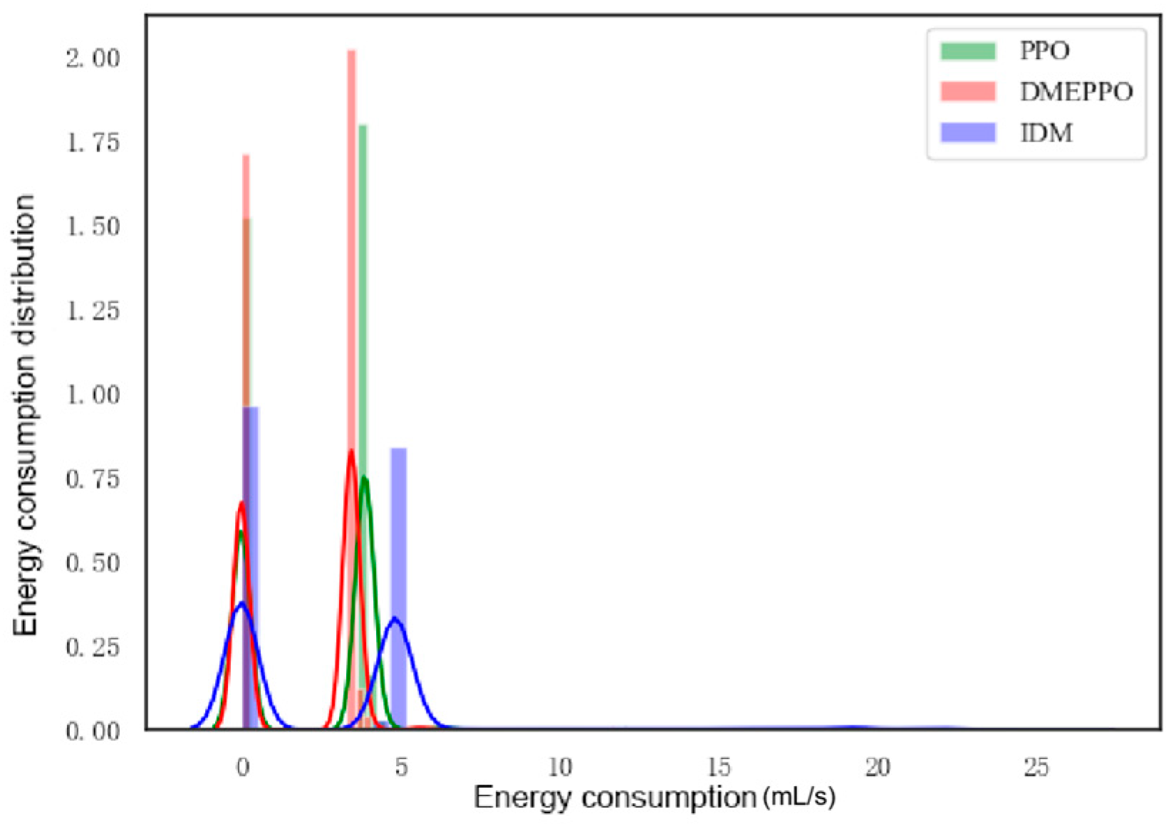
4.2.2. Consider Fuel Economy Rewards

Fuel efficiency is also a key factor to take into account. To minimize fuel consumption and save energy during unmanned agricultural vehicle operations, the reward function for fuel economy can be designed as

$$r_2=e^{-k_2\cdot Q_c}$$

(34)

where Q_c is the real-time fuel consumption of driverless agricultural vehicles and k₂ is an adjustable constant.

4.2.3. Consider the Rewards of Safety

When operating in the field, driverless agricultural vehicles inevitably encounter static or dynamic obstacles such as other operating machines, people, or hydraulic structures or rocks. Therefore, their front and rear safety distances from static and dynamic obstacles should be considered, and the reward function should be set as

$$r_3=-{\displaystyle \frac{1}{\min (d_f,d_r)+1}}$$

(35)

where d_f and d_r are the distances between the driverless agricultural vehicle and other obstacles in front of and behind it.

4.2.4. Consider the Rewards of Smooth Driving

The smoothness of driving is another factor to consider. Frequent acceleration and deceleration are detrimental to the reliability of a machine, as is excessive acceleration and deceleration, which reduce the life of the machine. Therefore, the reward function for the smoothness of driving is designed as

$$r_4=-{\displaystyle \frac{\max (\left|a_x\right|,\left|a_y\right|)}{10}}$$

(36)

where a_x and a_y are the longitudinal and lateral acceleration, respectively.

4.2.5. Multi-Objective Awards

Considering all the above reward aspects, the multi-objective reward function is established as

$$r={\displaystyle \frac{w_1}{{‖\mathit{w}‖}_1}}{r}_1+{\displaystyle \frac{w_2}{{‖\mathit{w}‖}_1}}{r}_2+{\displaystyle \frac{w_3}{{‖\mathit{w}‖}_1}}{r}_3+{\displaystyle \frac{w_4}{{‖\mathit{w}‖}_1}}{r}_4$$

(37)

where w_i denotes the weight of the above four reward objectives and i = 1, 2, 3, and 4. $\mathit{w}=\left[\begin{array}{cccc}{w}_1& w_2& w_3& w_4\end{array}\right]$ is a weight vector.

By adjusting the values of the weights, a decision can be made on the speed matching the demands of the dynamic environment. In this paper, focusing on the consideration of fuel economy, the weight vector was set as $\mathit{w}=\left[\begin{array}{cccc}1& 100& 1& 1\end{array}\right]$.

4.2.6. Network Settings

This study employed a four-layer neural network architecture, comprising an input layer, two hidden layers, and an output layer. Each of the hidden layers contains 128 neurons, powered by a rectified linear unit (ReLU) activation function. The network’s output provides the multi-objective-optimized speed for the autonomous agricultural vehicle. The input state of the neural network consists of 17 dimensions, as shown in

Table 1. Neural network input variables.

Serial Number	Variable	Input Meaning	Units
1	v0	The speed of the trained agricultural vehicle	m/s
2	v1	Speed of the machine in front of the agricultural vehicle	m/s
3	v2	Speed of the machine behind the agricultural vehicle	m/s
4	v3	Speed of the machine in front of and on the left side of the agricultural vehicle	m/s
5	v4	Speed of the machine behind and on the left side of the agricultural vehicle	m/s
6	v5	Speed of the machine to the right and in front of the agricultural vehicle	m/s
7	v6	Speed of the machine to the right and at the rear of the agricultural vehicle	m/s
8	ds1	Distance between agricultural vehicle and machine in front	m
9	ds2	Distance between agricultural vehicle and machine behind	m
10	ds3	Distance between the agricultural vehicle and the machine in front of it on the left-hand side	m
11	ds4	Distance between agricultural vehicle and machine to left and at rear	m
12	ds5	Distance between the agricultural vehicle and the machine in front of it on the right-hand side	m
13	ds6	Distance between agricultural vehicle and machine to the right and at rear	m
14	ni	Number of paths
15	as0	Training the longitudinal acceleration of the agricultural vehicle	m/s2
16	r0	Training the agricultural vehicle’s yaw speed	rad/s
17	mi	Agricultural vehicle operating mode weights

.

4.3. Design of LMI-Based Speed Tracking Controller

The objective of developing speed control for an autonomous agricultural vehicle was to develop a robust feedback controller. This controller calculates the control signal u(t) needed to ensure the system achieves asymptotic stability and meets H_∞ performance criteria in the presence of uncertainties and interference. The expression for this is as follows:

$${\displaystyle {\int }_0^t{z}^{\mathrm{T}}(t)z(t)dt\le {\rho }^2}{\displaystyle {\int }_0^t{w}^{\mathrm{T}}(t)w(t)dt}.$$

(38)

The robust feedback control law for this system can be designed as

$$u(t)=Ky(t)=K{C}_{1}x(t)$$

(39)

The velocity control model (15) can be converted to

$$\left\{\begin{array}{l}\dot{x}(t)=\tilde{A}x(t)+w(t)\hfill \\ z(t)=C_{2}x(t)\hfill \end{array}\right.$$

(40)

where $\tilde{A}=A+B{C}_{1}K$.

Two lemmas from the literature [29] are introduced to solve the above robust state feedback controller design problem.

Lemma 1.

In order to make the above closed-loop system asymptotically stable and satisfy the evaluation index, a positive ρ is given if and only if there exists a symmetric positive definite matrix, P, satisfying the following inequality:

$$\left[\begin{array}{ccc}\tilde{A}P+P{\tilde{A}}^{\mathrm{T}}& P& C_2^{\mathrm{T}}\\ \ast & -{\rho }^{2}I& 0\\ \ast & \ast & -I\end{array}\right]<0.$$

(41)

Lemma 2.

Given a positive definite matrix, $S=\left[\begin{array}{cc}{S}_{11}& S_{12}\\ S_{21}& S_{22}\end{array}\right]$, the following propositions are equivalent:

(1)

S < 0;

(2)

If S₁₁ < 0, then $S_{22}-S_{12}^{\mathrm{T}}{S}_{11}^{-1}{S}_{12}<0$;

(3)

If S₂₂ < 0, then $S_{11}-S_{12}{S}_{22}^{-1}{S}_{12}^{\mathrm{T}}<0$.

Since $\tilde{A}=A+B{C}_{1}K$, the following equation can be obtained:

$$\begin{array}{l}\tilde{A}P+P{\tilde{A}}^{\mathrm{T}}=(A+B{C}_{1}K)P+P{(A+B{C}_{1}K)}^{\mathrm{T}}\\ =AP+P{A}^{\mathrm{T}}+(EP+P{E}^{\mathrm{T}})\end{array}.$$

(42)

where E = BC₁K.

At the same time, the left-hand side of Equation (41) can be transformed into

$$\left[\begin{array}{ccc}\tilde{A}P+P{\tilde{A}}^{\mathrm{T}}& P& C_2^{\mathrm{T}}\\ \ast & -{\rho }^{2}I& 0\\ \ast & \ast & -I\end{array}\right]=\left[\begin{array}{ccc}AP+P{A}^{\mathrm{T}}& P& C_2^{\mathrm{T}}\\ \ast & -{\rho }^{2}I& 0\\ \ast & \ast & -I\end{array}\right]+{{\Gamma }_1}^{\mathrm{T}}{\Gamma }_2+{{\Gamma }_2}^{\mathrm{T}}{\Gamma }_3$$

(43)

where ${\Gamma }_1=\left[\begin{array}{ccc}E& 0& 0\end{array}\right]$, ${\Gamma }_2=\left[\begin{array}{ccc}P& 0& 0\end{array}\right]$, and ${\Gamma }_3=\left[\begin{array}{ccc}{E}^{\mathrm{T}}& 0& 0\end{array}\right]$.

Let $S_{11}=\left[\begin{array}{ccc}AP+P{A}^{\mathrm{T}}& P& C_2^{\mathrm{T}}\\ \ast & -{\rho }^{2}I& 0\\ \ast & \ast & -I\end{array}\right]$, $S_{12}={{\Gamma }_1}^{\mathrm{T}}{\Gamma }_2$, S₂₁ = S₁₂^T, and $S_{22}=\varpi diag\left\{I,I,I\right\}$,

where I is the unit vector.

According to Lemma 1 and Lemma 2, the following inequality can be derived:

$$\left[\begin{array}{cccccc}AP+P{A}^{\mathrm{T}}& P& C_2^{\mathrm{T}}& EP& 0& 0\\ \ast & -{\rho }^{2}I& 0& 0& 0& 0\\ \ast & \ast & -I& 0& 0& 0\\ \ast & \ast & \ast & -\varpi I& 0& 0\\ \ast & \ast & \ast & \ast & -\varpi I& 0\\ \ast & \ast & \ast & \ast & \ast & -\varpi I\end{array}\right]<0$$

(44)

given a positive constant, ρ, such that the closed-loop system (37) is asymptotically stable at w(t) = 0 if and only if there exist symmetric positive definite matrices, P, and scalars, $\varpi$, such that the above inequality holds while satisfying the H₂ performance metrics (38) and for all w(t) ∈ [0, ∞] cases.

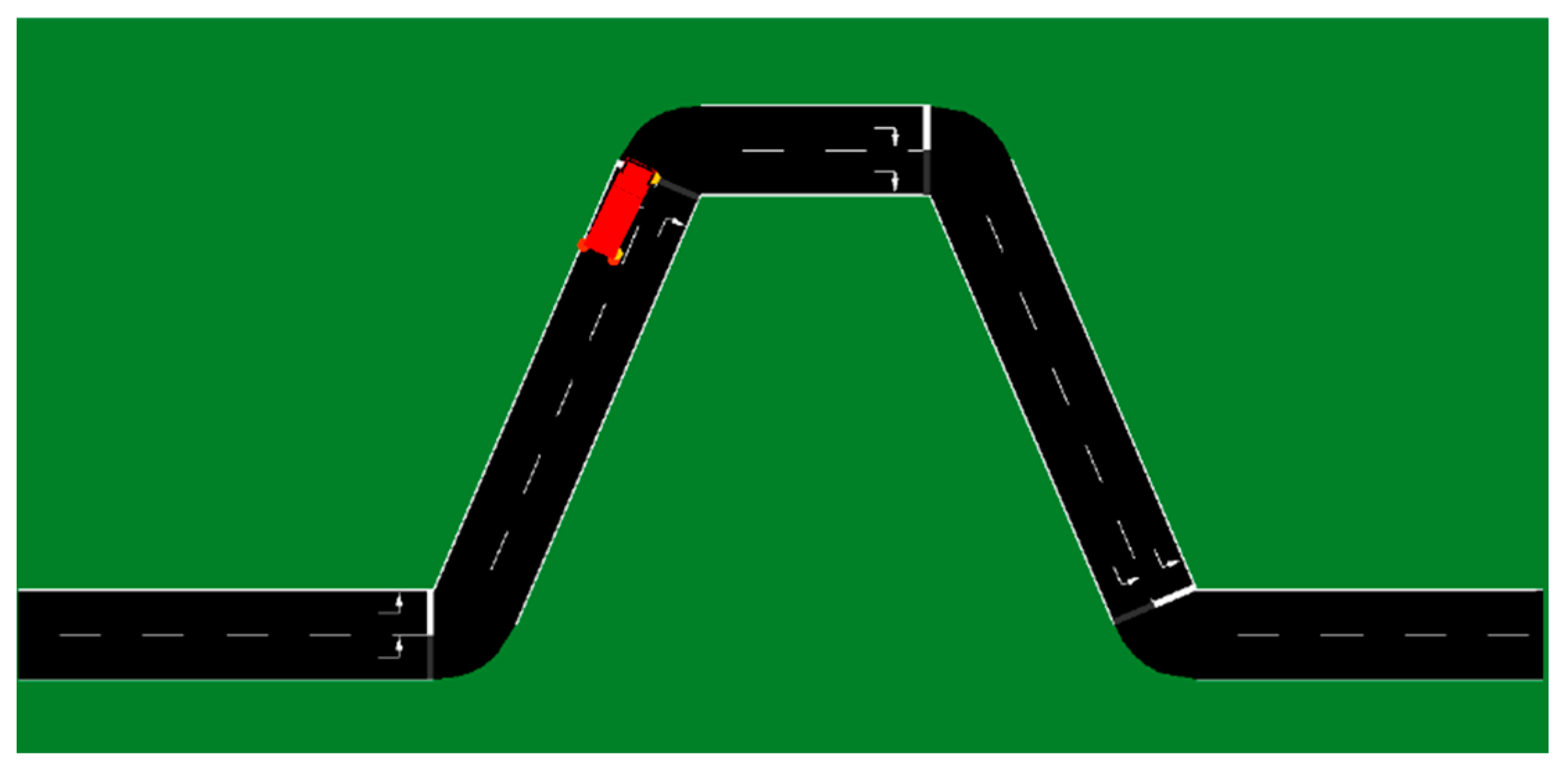
5. Experimental Method

A simulation test and HIL test were conducted to verify the proposed speed decision-making and control scheme for an unmanned agricultural vehicle. Figure 1 illustrates the speed decision-making and control scheme structure. The structure features a speed-determining layer using DMEPPO and an underlying speed tracking layer utilizing LMI-based robust control. The decision-making layer incorporates rewards aimed at enhancing efficiency, reducing fuel usage, and ensuring safety and the smoothness of travel. The training environment was based on Simulation of Urban Mobility 1.16.0 (SUMO, an open-source transportation simulation software system) [30]. Meanwhile, the five-degrees-of-freedom (5DOF) vehicle dynamic model, combined with the magic tire model, was embedded using SUMO, which effectively improved the dynamic characteristics of an agricultural vehicle, allowing for accurate simulations that more closely matched actual driving conditions and driving situations. The developed speed-determining model was tested in this specific environment to establish a reasonable speed. This model then enabled the agricultural vehicle to achieve its speed tracking objectives by maintaining the speed determined by the decision layer using an LMI-based tracking controller, thereby realizing multi-objective speed control for the agricultural vehicle.

In this section, we describe how the proposed hierarchical speed decision control method was simulated and validated. Firstly, the speed decision-making model was trained; then, the joint DRL module and speed robust control module were tested and validated. This training and testing simulation environment was based on SUMO. In order to make the simulation closer to a real situation, a five-degrees-of-freedom agricultural vehicle model and a tire model [31] were introduced into SUMO to increase the dynamic attributes of the agricultural vehicle. A double-shifted path was used for training and testing and is shown in Figure 2. Furthermore, to enhance the generalization capability and versatility of the trained artificial intelligence networks, these artificial intelligence networks were exposed to complex dynamic environments for testing, specifically by having them operate alongside a diverse array of vehicles in various operational conditions. For testing, an LMI speed control algorithm was developed in MATLAB^®2016, and its associated dynamic model was constructed using MATLAB/Simulink. To establish a link between the speed decision and control layers, the MATLAB Engine API for Python (3.5) was implemented and utilized, facilitating the comprehensive testing of the entire simulation setup [32].

6. Results and Discussion

In the simulation scenario of multi-vehicle cooperative operation, the main vehicle dynamically optimized the speed decision using the DMEPPO algorithm by acquiring the state information of the surrounding vehicles in real time (including the instantaneous speeds of and relative distances from the vehicles in the front and rear and on the left and right sides). Specifically, the input state of the main vehicle (shown in Table 1) included the parameters (such as v₁, v₂, d_s1, and d_s2) of the ambient vehicles collected using the on-board sensors and the communication module, and a comprehensive trade-off was performed based on the multi-objective reward function: when the vehicle ahead was detected as decelerating (v₁ decreased) or the safe distance decreased (d_s1 shortened), the safety reward term triggered the main vehicle to actively reduce its speed to maintain safe spacing, and when the rear vehicle accelerated (v₂ increased), the efficiency bonus term drove the main vehicle to increase its speed to match the speed of other vehicles partaking in the cooperative operation. In addition, the LMI controller dynamically adjusted the drive allocation under steering or road disturbances by robustly tracking the target speed output from the decision layer to ensure the smoothness of the speed change and the optimization of energy consumption.

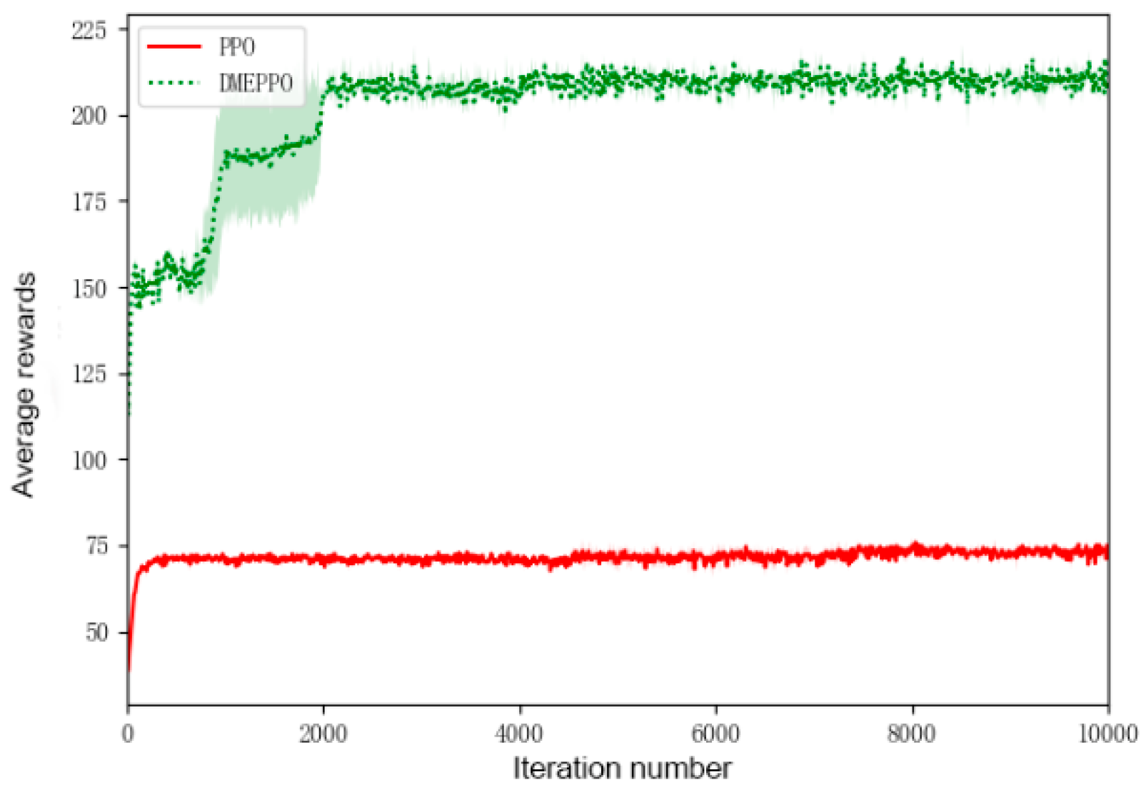
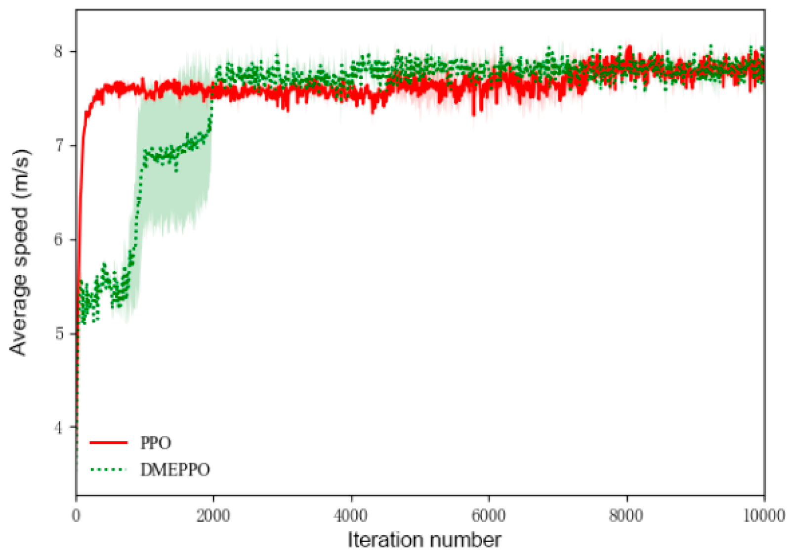
6.1. Speed Decision-Making Training Experiment

To conduct a thorough evaluation of the suggested DMEPPO longitudinal decision-making algorithm, training was executed with two distinct random seeds: 0 and 10,000. The results were compared with those from PPO training. Figure 3, Figure 4, Figure 5, Figure 6, Figure 7 and Figure 8 show the results of the training. The graphs were generated using the average data, with the shaded regions representing the minimum and maximum outcomes from the training process with different random seeds. At the same time, a reward score was set to represent the result of the intelligent vehicle interacting with the dynamic environment.

As can be seen from Figure 3, the system employing DMEPPO gradually reached convergence and stability at 2000 steps with a score of about 210 and experienced two jumps out of the local optimum at about 800 and 2000 steps, which illustrates the fact that with the introduction of the entropy constraints, the system employing DMEPPO had a better exploratory capability and thus achieved a final score of over 200. In contrast, the system using PPO was trained to obtain a locally optimal result at the beginning and increasingly favored that result, which ultimately led to a locally optimal strategy being obtained, and its final score was 75.

Figure 4 shows the agricultural vehicle’s speed trajectory during training. Since we set the maximum driving speed of the agricultural vehicle to 8 m/s during training and gave the speed-related operational efficiency the highest weight, both the system employing DMEPPO and the system employing PPO gradually converged to the highest operational efficiency of 8 m/s.

From Figure 5 and Figure 6, it can be seen that with an increase in the velocity, the longitudinal acceleration improved under DMEPPO and PPO and increased gradually from 0 to 0.025 m/s², while the value of the lateral acceleration converged gradually from −2.0 m/s² to about 0 and ultimately reached an equilibrium state at the highest score.

Figure 7 shows the energy consumption training curves, and it can be seen that as the number of training steps increased, both the system employing DEMPPO and the system employing PPO were gradually trained to achieve the minimum energy consumption of 3 mL/s after accounting for trade-offs, but the system employing DEMPPO performed more consistently.

As can be seen from Figure 8, the system employing PPO had a high number of collisions from the beginning to the end, indicating that the PPO algorithm had not learnt how to make the driverless agricultural vehicle travel more safely. The number of collisions for the system employing DMEPPO gradually increased from 3 at the beginning to about 12, mainly because we set the operational efficiency mode so that it pursued a higher traveling speed, which made the traveling safe a “sacrifice”.

The above training results show that the introduction of maximum entropy-constrained proximal policy optimization could make the training process converge more quickly. The training process could proceed more stably with different random seeds.

6.2. Speed Decision-Making Test Experiment

After training, a suitable DMEPPO-based speed decision-making model was obtained, which needed to be tested for its real-world effectiveness. Since the Intelligent Driving Model (IDM) is a rule-based model inbuilt in SUMO, the IDM was chosen as an alternative to PPO to provide a comparison. In order to test the adaptive ability of the speed decision-making models trained using different strategies—the DMEPPO and PPO models and the IDM—in dynamic environments, various types of dynamic obstacles were set up in the test environment. Figure 9, Figure 10, Figure 11, Figure 12 and Figure 13 show Kernel Density Estimations which show the distribution characteristics of the test data. The interpretation of kernel density maps mainly relies on the shape and distribution of the curves. The curve in a kernel density map represents the probability density estimation of the data. The higher the curve, the higher the density of the data point at that position.

As can be seen in Figure 9, the DMEPPO model’s reward scores were high, with the reward scores concentrated around 105. Both the PPO model and IDM’s scores were low, with the PPO model’s mainly distributed between 35 and 40 and the IDM’s mainly distributed between 65 and 80. This indicates that the speed control strategy developed exhibited a certain level of dynamic responsiveness.

From Figure 10, it can be seen that the longitudinal velocities obtained using the DMEPPO and PPO models were mainly concentrated around 3–4 m/s due to balance considerations, while the IDM has a rule-based design, and the velocity distribution was mostly around the set limit value of 8 m/s. From Figure 11 and Figure 12, it can be observed that the longitudinal accelerations for the three approaches were largely centered around 0 m/s², i.e., the vehicle tended to travel at a longitudinal uniform speed to keep the driving smooth. In order to examine the lateral stability of the unmanned agricultural vehicle, the driving path in this paper was set up as a double-shifted line. Under PPO and DMEPPO, the lateral acceleration was −4 m/s² and −3 m/s², respectively, while using the IDM it reached ±10 m/s², which very easily caused lateral instability and was also due to the over-pursuit of efficiency of the IDM.

From Figure 13, it can be seen that the energy consumption under both DMEPPO and PPO was lower than when using the IDM, mainly concentrated around 4 mL/s, and both of these strategies maintained the balance of energy consumption, with DMEPPO consuming slightly less energy and being the most energy-efficient. The IDM consumed the highest amount of energy, up to 5 mL/s, and it achieved high efficiency at the cost of higher energy consumption.

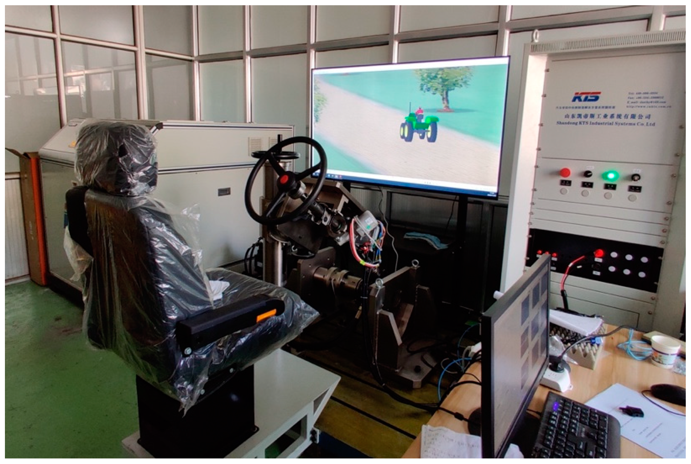
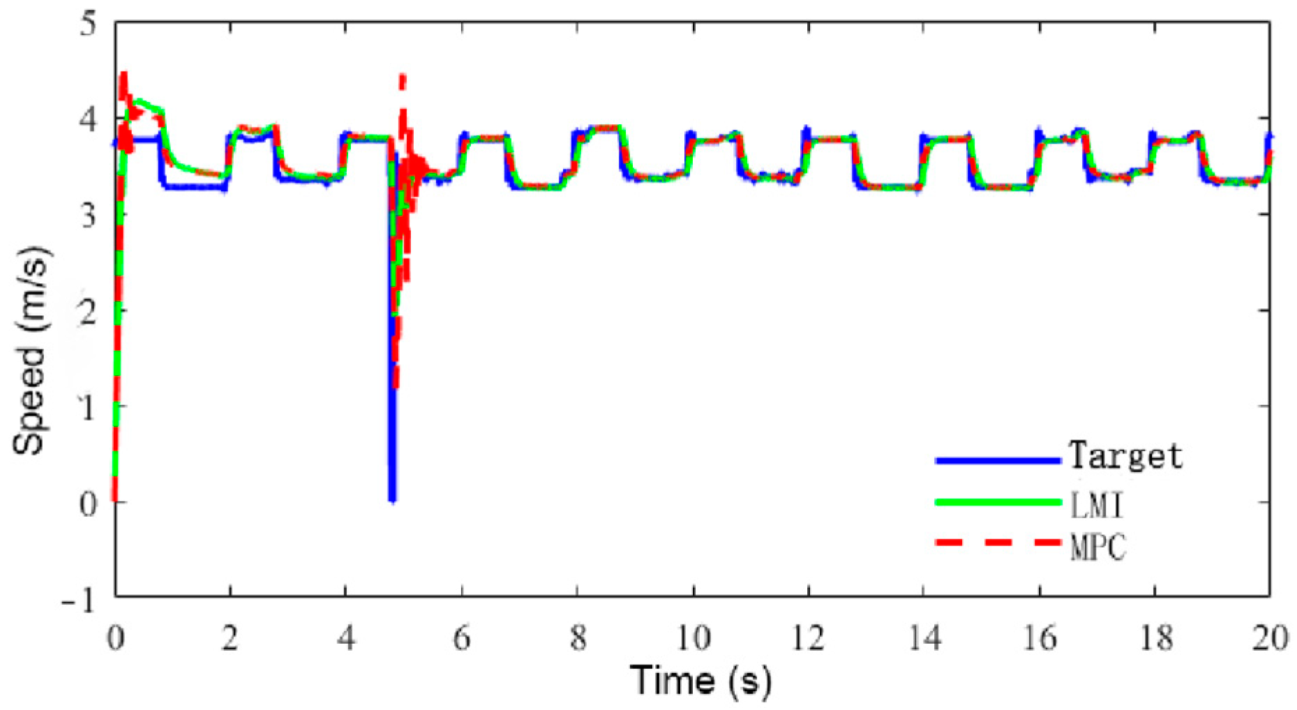
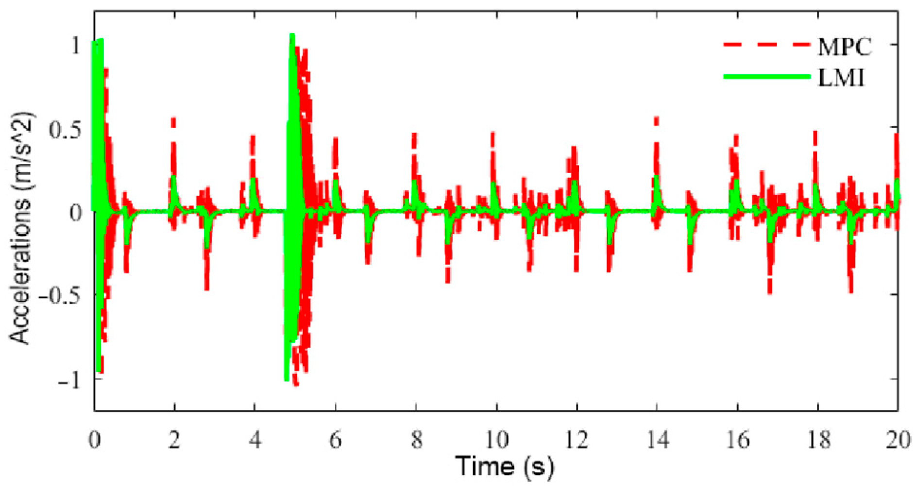
6.3. Speed Tracking Control HIL Simulation Test

To assess the speed tracking performance, particularly the robustness of the proposed LMI control approach, an HIL experiment was conducted. The HIL experiment bench built in this study is shown in Figure 14, and it was composed of a steering system, steering resistance loading system, a dSPACE Microautobox and an NI PXI. A simulation comparing speed control using model predictive control (MPC) was conducted at the same time. The MPC sampling time was set to 0.01 s, and the simulation outcomes are depicted in Figure 15, Figure 16, Figure 17 and Figure 18.

The speed limits for the MPC-based constraints were tied to the speed of the unmanned agricultural vehicle, extending from 0 to 8 m/s. The primary goals of MPC are to reduce tracking errors and disturbances while constraining the control inputs, so the weight matrix was set as $Q_{MPC}=diag\left[\begin{array}{ccc}0.6& 0.2& 0.3\end{array}\right]$.

As shown in Figure 15, the blue curve is the target speed obtained by DMEPPO. Each test step exhibited clear acceleration and deceleration phases at its onset and conclusion. In addition, the sharp change in the velocity at each step can be regarded as an uncertainty or disturbance. Both MPC and LMI-based control could track the target velocity. Compared to MPC, LMI-based control had better stability when the velocity increased sharply.

As can be seen from Figure 16, the acceleration with LMI-based control was within −0.2–0.2 m/s², and the velocity control was smoother, while the acceleration with MPC was generally within −0.5–0.5 m/s², and the acceleration was larger, and at the same time, velocity control based on MPC significantly lagged behind that based on LMIs when acceleration and deceleration control was carried out, which indicates that LMI-based control had a better response capability than MPC. From Figure 17, it can be seen that compared with MPC, the speed tracking control achieved with LMIs consumed less energy.

Figure 18 shows a comparison of the driving torque of the agricultural vehicle’s rear drive wheels when using the MPC and LMI controllers. The driving torque with MPC was significantly higher than that with LMI-based control, with greater fluctuations. In addition, the output torque with LMI-based control was greater than that with MPC, which proves that the designed speed controller has good robustness, stability, and response performance.

7. Conclusions

This paper proposes a robust speed decision control method for unmanned agricultural vehicles. It integrates DRL with robust control techniques. The method employs a hierarchical decision control architecture. Firstly, based on PPO, the DMEPPO optimal speed decision-making algorithm was designed by considering dynamic environment information and introducing heuristic goal entropy and adaptive entropy constraints. In order to obtain a more dynamically adaptive learning model, a multi-objective setting reward function was considered. Secondly, an LMI controller, which accounted for uncertainties and disturbances, was developed to track the decided speed derived from the decision-making layer. Thus, the entire process of speed decision-making and tracking control was implemented. The simulation test and HIL results show that the proposed speed decision-making and control scheme for unmanned agricultural vehicles is feasible and effective, and our findings can be summarized as follows:

(1)

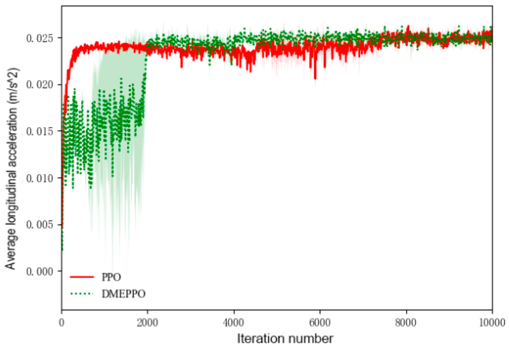
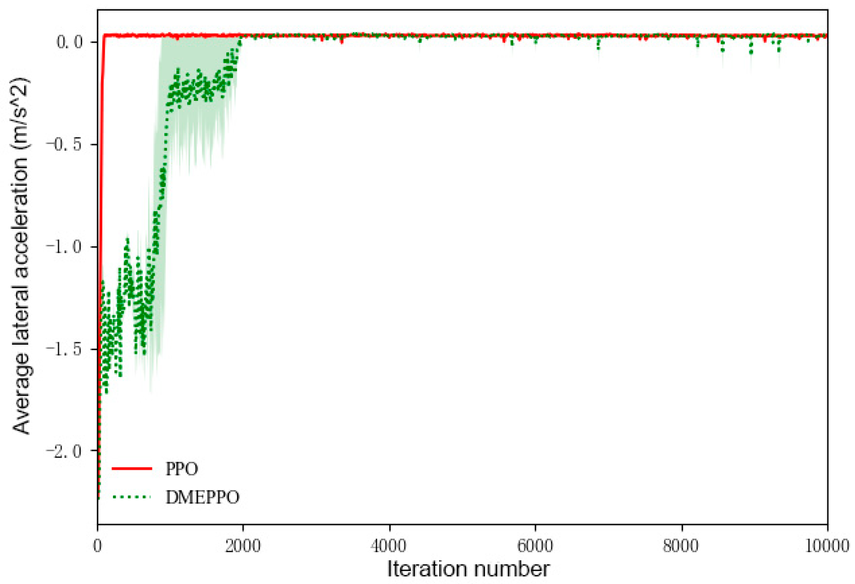
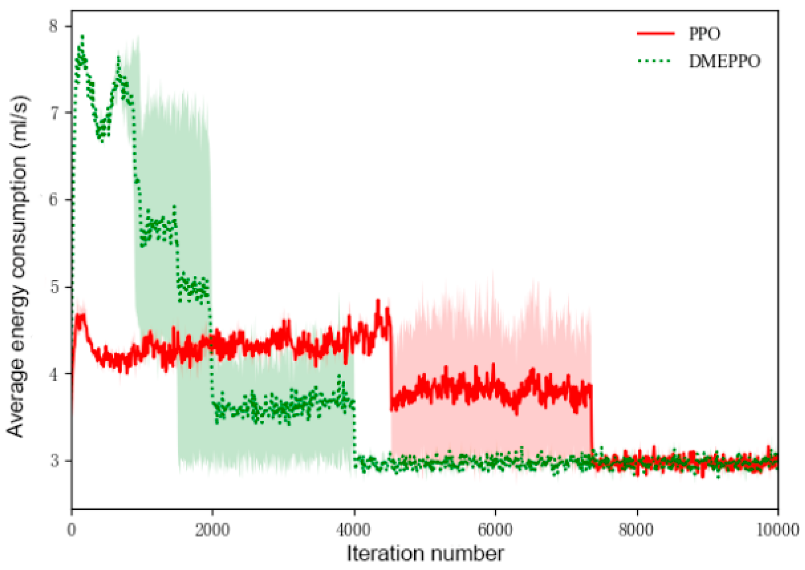
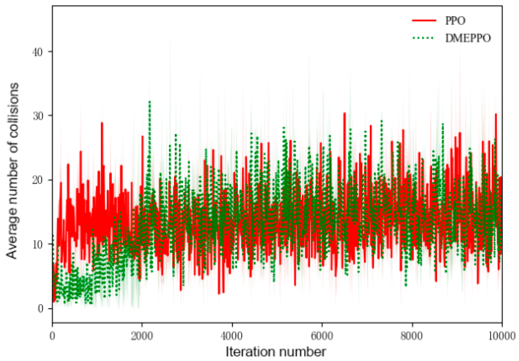
It could be seen from the training and testing of the DMEPPO speed decision-making strategy that the trained speed decision-making model is able to converge quickly within 2000 iterations and was able to complete decision-making when facing multi-objective tasks in the test.

(2)

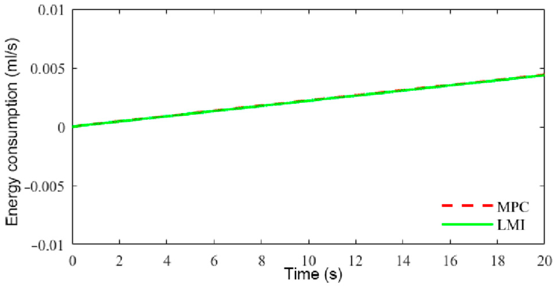
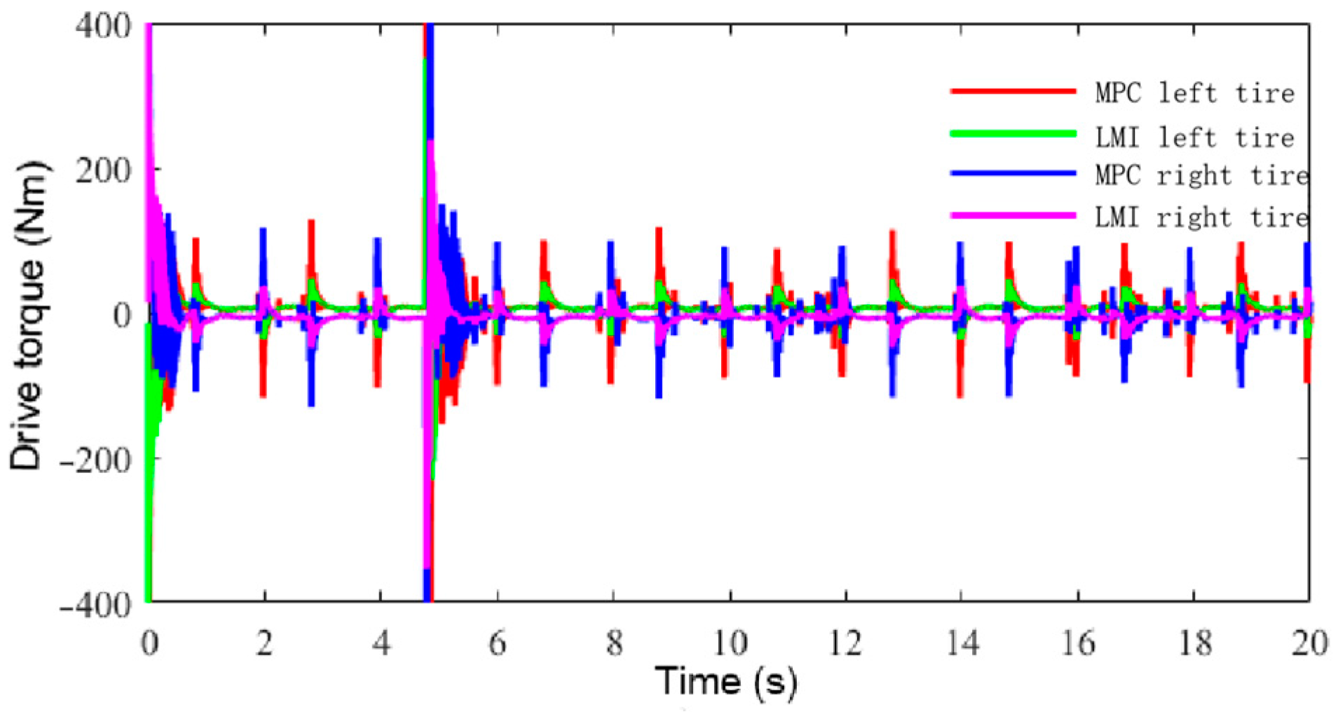
The suggested LMI-based speed controller effectively maintained the robust tracking of the intended speed amidst uncertainty and disturbances. The comprehensive performance of the controller resulted in robustness to uncertainties and disturbances, smooth driving with frequent acceleration and deceleration, low power consumption, and good output responsiveness.

The current work has laid the foundation for single-vehicle control, and in the future, it can be expanded to a multi-vehicle information flow topology and distributed control.

References

1. Chen, Z.; Lai, J.; Li, P.; Awad, O.I.; Zhu, Y. Prediction horizon-varying model predictive control (MPC) for autonomous vehicle control. Electronics 2024, 13, 1442. [Google Scholar] [CrossRef]
2. Zhao, S.; Leng, Y.; Shao, Y. Explicit model predictive control of multi-objective adaptive cruise of vehicle. J. Transp. Eng. 2020, 20, 206–216. [Google Scholar]
3. Moser, D.; Schmied, R.; Waschl, H.; del Re, L. Flexible spacing adaptive cruise control using stochastic model predictive control. IEEE Trans. Control Syst. Technol. 2017, 26, 114–127. [Google Scholar] [CrossRef]
4. Jin, J.; Li, Y.; Huang, H.; Dong, Y.; Liu, P. A variable speed limit control approach for freeway tunnels based on the model-based reinforcement learning framework with safety perception. Accid. Anal. Prev. 2024, 201, 107570. [Google Scholar] [CrossRef]
5. Zhang, Y.; Li, J.; Zhou, H.; Chng, C.B.; Chui, C.K.; Zhao, S. Comprehensive evaluation of deep reinforcement learning for permanent magnet synchronous motor current tracking and speed control applications. Eng. Appl. Artif. Intell. 2025, 149, 110551. [Google Scholar] [CrossRef]
6. Goodall, N.J.; Lan, C.L. Car-following characteristics of adaptive cruise control from empirical data. J. Transp. Eng. Part A Syst. 2020, 146, 04020097. [Google Scholar] [CrossRef]
7. Melson, C.L.; Levin, M.W.; Hammit, B.E.; Boyles, S.D. Dynamic traffic assignment of cooperative adaptive cruise control. Transp. Res. Part C Emerg. Technol. 2018, 90, 114–133. [Google Scholar] [CrossRef]
8. Liu, H.; Wang, H.; Niu, K.; Zhu, R.; Zhang, Z. Research on car-following models and platoon speed guidance based on real datasets in connected and automated environments. Transp. Lett. 2025, 1–15. [Google Scholar] [CrossRef]
9. Wang, C.; Gong, S.; Zhou, A.; Li, T.; Peeta, S. Cooperative adaptive cruise control for connected autonomous vehicles by factoring communication-related constraints. Transp. Res. Part C Emerg. Technol. 2020, 113, 124–145. [Google Scholar] [CrossRef]
10. Li, T.; Chen, D.; Zhou, H.; Laval, J.; Xie, Y. Car-following behavior characteristics of adaptive cruise control vehicles based on empirical experiments. Transp. Res. Part B Methodol. 2021, 147, 67–91. [Google Scholar] [CrossRef]
11. You, Z. Design of automotive mechanical automatic transmission system based on torsional vibration reduction. J. Vibroeng. 2023, 25, 683–697. [Google Scholar] [CrossRef]
12. Geng, G.; Jiang, F.; Chai, C.; Wu, J.; Zhu, Y.; Zhou, G.; Xiao, M. Design and experiment of magnetic navigation control system based on fuzzy PID strategy. Mech. Sci. 2022, 13, 921–931. [Google Scholar] [CrossRef]
13. Wang, L.; Li, L.; Wang, H.; Zhu, S.; Zhai, Z.; Zhu, Z. Real-time vehicle identification and tracking during agricultural master-slave follow-up operation using improved YOLO v4 and binocular positioning. Proc. Inst. Mech. Eng. Part C J. Mech. Eng. Sci. 2023, 237, 1393–1404. [Google Scholar] [CrossRef]
14. Chu, L.; Li, H.; Xu, Y.; Zhao, D.; Sun, C. Research on longitudinal control algorithm of adaptive cruise control system for pure electric vehicles. World Electr. Veh. J. 2023, 14, 32. [Google Scholar] [CrossRef]
15. Mehraban, Z.; Zadeh, A.Y.; Khayyam, H.; Mallipeddi, R.; Jamali, A. Fuzzy adaptive cruise control with model predictive control responding to dynamic traffic conditions for automated driving. Eng. Appl. Artif. Intell. 2024, 136, 109008. [Google Scholar] [CrossRef]
16. Yin, X.; Wang, Y.; Chen, Y.; Jin, C.; Du, J. Development of autonomous navigation controller for agricultural vehicles. Int. J. Agric. Biol. Eng. 2020, 13, 70–76. [Google Scholar] [CrossRef]
17. Wu, Z.; Xie, B.; Li, Z.; Chi, R.; Ren, Z.; Du, Y.; Inoue, E.; Mitsuoka, M.; Okayasu, T.; Hirai, Y. Modelling and verification of driving torque management for electric tractor: Dual-mode driving intention interpretation with torque demand restriction. Biosyst. Eng. 2019, 182, 65–83. [Google Scholar] [CrossRef]
18. Saeed, M.A.; Ahmed, N.; Hussain, M.; Jafar, A. A comparative study of controllers for optimal speed control of hybrid electric vehicle. In Proceedings of the 2016 International Conference on Intelligent Systems Engineering (ICISE), Islamabad, Pakistan, 15–17 January 2016; IEEE: New York, NY, USA, 2016; pp. 1–4. [Google Scholar]
19. Zhu, M.; Chen, H.; Xiong, G. A model predictive speed tracking control approach for autonomous ground vehicles. Mech. Syst. Signal Process. 2017, 87, 138–152. [Google Scholar] [CrossRef]
20. Tanaka, T.; Nakayama, S.; Wasa, Y.; Hirata, K.; Hatanaka, T. A continuous-time primal-dual algorithm with convergence speed guarantee utilizing constraint-based control. SICE J. Control. Meas. Syst. Integr. 2025, 18, 2485496. [Google Scholar] [CrossRef]
21. He, X.; Fei, C.; Liu, Y.; Yang, K.; Ji, X. Multi-objective longitudinal decision-making for autonomous electric vehicle: A entropy-constrained reinforcement learning approach. In Proceedings of the 2020 IEEE 23rd International Conference on Intelligent Transportation Systems (ITSC), Rhodes, Greece, 20–23 September 2020; IEEE: New York, NY, USA, 2020; pp. 1–6. [Google Scholar]
22. Xiao, B.; Yang, W.; Wu, J.; Walker, P.D.; Zhang, N. Energy management strategy via maximum entropy reinforcement learning for an extended range logistics vehicle. Energy 2022, 253, 124105. [Google Scholar] [CrossRef]
23. He, X.; Huang, W.; Lv, C. Trustworthy autonomous driving via defense-aware robust reinforcement learning against worst-case observational perturbations. Transp. Res. Part C Emerg. Technol. 2024, 163, 104632. [Google Scholar] [CrossRef]
24. He, X.; Hao, J.; Chen, X.; Wang, J.; Ji, X.; Lv, C. Robust Multiobjective Reinforcement Learning Considering Environmental Uncertainties. IEEE Trans. Neural Netw. Learn. Syst. 2024, 36, 6368–6382. [Google Scholar] [CrossRef] [PubMed]
25. Tang, C.Y.; Liu, C.H.; Chen, W.K.; You, S.D. Implementing action mask in proximal policy optimization (PPO) algorithm. ICT Express 2020, 6, 200–203. [Google Scholar] [CrossRef]
26. Liang, J.; Feng, J.; Fang, Z.; Lu, Y.; Yin, G.; Mao, X.; Wu, J.; Wang, F. An energy-oriented torque-vector control framework for distributed drive electric vehicles. IEEE Trans. Transp. Electrif. 2023, 9, 4014–4031. [Google Scholar] [CrossRef]
27. Feng, J.; Yin, G.; Liang, J.; Lu, Y.; Xu, L.; Zhou, C.; Peng, P.; Cai, G. A Robust Cooperative Game Theory based Human-machine Shared Steering Control Framework. IEEE Trans. Transp. Electrif. 2023, 10, 6825–6840. [Google Scholar] [CrossRef]
28. Bui, V.H.; Mohammadi, S.; Das, S.; Hussain, A.; Hollweg, G.V.; Su, W. A critical review of safe reinforcement learning strategies in power and energy systems. Eng. Appl. Artif. Intell. 2025, 143, 110091. [Google Scholar] [CrossRef]
29. Park, I.S.; Park, C.E.; Kwon, N.K.; Park, P. Dynamic output-feedback control for singular interval-valued fuzzy systems: Linear matrix inequality approach. Inf. Sci. 2021, 576, 393–406. [Google Scholar] [CrossRef]
30. Thabet, A.S.M.; Zengin, A. Optimizing Dijkstra’s Algorithm for Managing Urban Traffic Using Simulation of Urban Mobility (Sumo) Software. Ann. Math. Phys. 2024, 7, 206–213. [Google Scholar]
31. Xu, G.; Chen, M.; He, X.; Liu, Y.; Wu, J.; Diao, P. Research on state-parameter estimation of unmanned Tractor—A hybrid method of DEKF and ARBFNN. Eng. Appl. Artif. Intell. 2024, 127, 107402. [Google Scholar] [CrossRef]
32. Naseri, K.; Vu, M.T.; Mobayen, S.; Najafi, A.; Fekih, A. Design of linear matrix inequality-based adaptive barrier global sliding mode fault tolerant control for uncertain systems with faulty actuators. Mathematics 2022, 10, 2159. [Google Scholar] [CrossRef]
Figure 1. Speed decision-making and control principles block diagram.
Sustainability 17 04326 g001
Figure 2. Double-shifted path.
Sustainability 17 04326 g002
Figure 3. Training score.
Sustainability 17 04326 g003
Figure 4. Average speed during training.
Sustainability 17 04326 g004
Figure 5. Average longitudinal acceleration during training.
Sustainability 17 04326 g005
Figure 6. Average lateral acceleration during training.
Sustainability 17 04326 g006
Figure 7. Average energy consumption during training.
Sustainability 17 04326 g007
Figure 8. Average number of training collisions.
Sustainability 17 04326 g008
Figure 9. Score distribution in test.
Sustainability 17 04326 g009
Figure 10. Velocity distribution in test.
Sustainability 17 04326 g010
Figure 11. Longitudinal acceleration distribution in test.
Sustainability 17 04326 g011
Figure 12. Lateral acceleration distribution in test.
Sustainability 17 04326 g012
Figure 13. Power consumption distribution in test.
Sustainability 17 04326 g013
Figure 14. HIL test bench.
Sustainability 17 04326 g014
Figure 15. Diagram of speed decision-making and control results for different controllers.
Sustainability 17 04326 g015
Figure 16. Acceleration with different tracking controllers at different speeds.
Sustainability 17 04326 g016
Figure 17. Power consumption with different tracking controllers at different speeds.
Sustainability 17 04326 g017
Figure 18. Driving torques with different tracking controllers at different speeds.
Sustainability 17 04326 g018